Simulation of Claylike Colloids
Abstract
Abstract. We investigate properties of dense suspensions and sediments of small spherical silt particles by means of a combined Molecular Dynamics (MD) and Stochastic Rotation Dynamics (SRD) simulation. We include van der Waals and effective electrostatic interactions between the colloidal particles, as well as Brownian motion and hydrodynamic interactions which are calculated in the SRD-part. We present the simulation technique and first results. We have measured velocity distributions, diffusion coefficients, sedimentation velocity, spatial correlation functions and we have explored the phase diagram depending on the parameters of the potentials and on the volume fraction.
pacs:
82.70.-y 47.11.+j, 05.40.-a, 02.70.NsI Introduction
We simulate claylike colloids, for which in many cases the attractive Van-der-Waals forces are relevant. They are often called “peloids” (Greek: clay-like). The colloidal particles have diameters in the range of some nm up to some m. In general, colloid science is a large field, where many books have been published Mahanty and Ninham (1996); Lagaly et al. (1997); Shaw (1992); Morrison and Ross (2002); Schmitz (1993); Hunter (2001). The term “peloid” originally comes from soil mechanics, but particles of this size are also important in many engineering processes. Our model system of Al2O3-particles of diameter m suspended in water is an often used ceramics and plays an important role in technical processes. In soil mechanicsRichter and Huber (2003) and ceramics scienceOberacker et al. (2001), questions on the shear viscosity and compressibility as well as on porosity of the microscopic structure which is formed by the particles, ariseWang et al. (1999); Lewis (2000). In both areas, usually high volume fractions () are of interest. The mechanical properties of these suspensions are difficult to understand. Apart from the attractive forces, electrostatic repulsion strongly determines the properties of the suspension. Depending on the surface potential, which can be adjusted by the pH-value of the solvent, one can either observe formation of clusters or the particles are stabilized in suspension and do sediment only very slowly. Hydrodynamic effects are also important for sedimentation experiments. Since typical Peclet numbers are of order one in our system, Brownian motion cannot be neglected.
In summary, there are many important factors which have to be included into a model which describes peloids
in a satisfying way. Such a model is needed to gain a deeper understanding of the dynamics of
dense colloidal suspensions. A lot of effort has been invested by
applying different simulation methods, which have their inherent
strengths but also some disadvantages.
Simplified Brownian Dynamics (BD), such as in the work of
Hütter Hütter (2000) does not contain long-ranged hydrodynamic
interactions among particles at all.
The computational cost is low, since hydrodynamics is reduced to a
simple Stokes force and thus large particle numbers can be handled.
BD with full hydrodynamic interactions utilizes a mobility matrix which
is based on the Oseen- or Rotne-Prager-Yamakawa tensor approximations
which are exact in the limit of zero Reynolds number and zero particle
volume fractionPetera and Muthukumar (1999); Ahlrichs et al. (2001).
This technique faces the main problem that the computational effort
scales with the cube of the particle number due to the inversion of
matrices.
The lattice Boltzmann (LB) method on the other hand is numerically
efficient and intrinsically contains hydrodynamic interactions. Ladd and
Verberg give an overview over the LB method and describe how to include
stress fluctuations Ladd and Verberg (2001). Adhikari et al. add noise to their
model by introducing a noise term for every lattice velocity and node
Adhikari et al. (2005). However, the discussion about the correct inclusion of
thermal fluctuations is still ongoing Adhikari et al. (2005); Usta et al. (2005).
Pair-Drag simulations have been proposed by Silbert et al.L.E. Silbert et al. (1997),
which include hydrodynamic interactions in an approximative way. They have focused on suspensions with
high densities (up to ) of uncharged spherical colloidal particles.
Here we use Stochastic Rotation Dynamics (SRD)Malevanets and Kapral (1999, 2000), a recently developed method
to simulate fluid flow, and combine this with a Molecular Dynamics (MD) simulation
for the suspended particles. SRD is a particle-based method which does
not show any numerical instabilities, contains thermal fluctuations
intrinsically and is simple to implement. Many important issues in
fluctuation fluid dynamics such as sedimentation Padding and Louis (2004),
vesicles in flow Noguchi and Gompper (2004), polymers in flow Ali et al. (2004),
reacting fluids Tucci and Kapral (2004) have been addressed very recently using
this method.
In this paper, first we discuss the main points of the MD-part of our simulation code, second
we present the SRD method in the context of our work, then we describe two alternative
ways of coupling the two parts of the simulation and point out the advantages
and disadvantages of these two possibilities. After that, we analyze the time
scales which are relevant for the peloids, we want to simulate. Based on the
insights of this section we show in the following section how to determine
the simulation parameters. Then we describe how we have tested our simulation
code and present first results in the following section. Finally in the last
section we draw a conclusion and summarize shortly the model we have presented.
II Molecular Dynamics
The colloidal particles in our simulation are represented by three dimensional spheres. In order to correctly model the statics and dynamics when approaching stationary states, realistic potentials are needed. The interaction between the particles is described by DLVO theoryHütter (2000); Russel et al. (1995); Lewis (2000). If the colloidal particles are suspended in a solvent, typically water, ions move into solution, whereas their counter ions remain in the particle due to a different resolvability. Thus, the colloidal particle carries a charge. The ions in solution are attracted by the charge on the particles and form the electric double layer. It has been shown (see Russel et al. (1995)), that the resulting electrostatic interaction between two of these particles can be described by an exponentially screened Coulomb potential
| (1) |
where denotes the particle diameter and is the distance of the particle centers. is the charge of the ions, the elementary charge, the temperature, denotes the effective surface potential, and is the inverse Debye screening length. In addition the behavior is determined by the attractive van der Waals interaction which can analytically be integrated over the two spheres. This leads to the second part of the DLVO potential:
| (2) |
is the Hamaker constant which involves the polarizability of the particles and of the solvent. The DLVO potentials are plotted in Fig. 1 for six typical examples with different depth of the secondary minimum. The primary minimum has to be modeled separately, as discussed below.

To avoid that the particles penetrate each other, one needs a repulsive force depending on their overlap. We are using a Hertz force described by the potential
| (3) |
where could be expressed by the elastic modulus of Al2O3. This would determine
the simulation time step, but to keep computational effort relatively small, we determine
the time step using the DLVO-potentials as described later on and then choose a value for
. Two aspects have to be considered: has to be big enough so that the particles
do not penetrate each other by more than approximately and it may not be too big, so that
numerical errors are kept small, which is the case when the collision time is resolved
with about 20 time steps. Otherwise total energy and momentum are not conserved very well
in the collision.
Since DLVO theory contains the assumption of linear polarizability, it holds only for
large distances, i.e. the singularity when the two spheres touch, does not exist in reality.
Nevertheless, there is an energy minimum about deep, so that
particles which come that close would very rarely become free again. To obtain numerical
stability of our simulation, we model this minimum by a parabolic potential, some
deep (e.g. ).
The depth of the minimum in our model is much less than in reality, but the probability
for particles to be trapped in the minimum has to be kept low enough so that only few
of them might escape during simulation time.
Long range hydrodynamic interaction is taken into account in a separate simulation for
the fluid as described below. This can only reproduce interactions correctly down
to a certain level. On shorter distances, a lubrication force has to be
introduced explicitly in the molecular dynamics simulation as described in Schwarzer (1995).
The most dominant mode, the so-called squeezing mode, is an additional force
| (4) | |||||
| (5) |
between two spheres with radii , and the relative velocity .
is the dynamic viscosity of the fluid.
diverges if particles touch each other.
Therefore, we limit the force by introducing a minimum radius,
where the force reaches its largest allowed value. The potential is shifted accordingly to smaller
particle distances, so that the maximum force is reached for particles touching each other.
The Hertz force also contains a damping term in normal direction,
| (6) |
with a damping constant and for the transverse direction a viscous friction proportional to the relative velocity of the particle surfaces is applied.
For the integration of the translational motion we utilize a velocity Verlet algorithmAllen and Tildesley (1987) chap. 3.2.1 to update the velocity and position of particle according to the equations
| (7) | |||||
| (8) |
For the rotation, a simple Euler algorithm is applied:
| (9) | |||||
| (10) |
where is the angular velocity of particle at time , is
the torque exerted by non central forces on the particle , is the orientation
of particle at time , expressed by a quaternion, and
gives the evolution of of particle rotating with the angular velocity
at time .
The concept of quaternionsAllen and Tildesley (1987) is often used to calculate rotational motions in simulations,
because the Euler angles and rotation matrices can easily be derived from quaternions. Using Euler angles
to describe the orientation would give rise to singularities for the two orientations
with . The numerical problems related to this fact and the relatively high
computational effort of a matrix inversion can be avoided using quaternions.
We have switched off dissipative forces and checked if the total energy and
each component of the total momentum are conserved. We have verified this for the molecular
dynamics simulation for the simulation of the fluid, and for the coupled simulation separately.
We also checked that our implementation of the molecular dynamics code is correct by
simulating eight large particles with Hertz-repulsion and Coulomb friction in a closed box
at a volume fraction of . We checked that the collisions are
realistic, i.e. that the individual angular velocities for two particles interacting in a
non-central collision before and after they have touched are consistent.
III Stochastic Rotation Dynamics (SRD): Simulation of the Fluid
The Stochastic Rotation Dynamics method (SRD) introduced by Malevanets and Kapral Malevanets and Kapral (1999, 2000)
is a promising tool for a coarse-grained description of
a fluctuating solvent, in particular for colloidal and polymer suspensions. The method is also
known as “Real-coded Lattice Gas” Inoue et al. (2002) or as “multi-particle-collision dynamics” (MPCD)
Ripoll et al. (2004).
It can be seen as a “hydrodynamic heat bath”, whose details are not fully resolved but which
provides the correct hydrodynamic interaction among embedded particlesLamura et al. (2001).
SRD is especially well suited for flow problems with Peclet numbers of
order one and Reynolds numbers on the particle scale between 0.05 and 20
for ensembles of many particles111For low Peclet numbers Brownian motion dominates and sedimentation takes place very slowly.
The simulations require a huge number of time steps.
Then Brownian simulation (BS), including short range hydrodynamics interactions, might be a more suitable
tool, since not the complete velocity field has to be calculated. For very high Peclet numbers,
SRD becomes inefficient due to the necessary averaging. For high Reynolds numbers a
small time step and high spacial resolution would be necessary, which increases the computational
effort extremely..
The numerical effort scales linearly with the number of embedded
colloidal particles unlike in Brownian Dynamics, and only one random
number per node (for the choice of the rotation matrix) is needed in
contrast to fluctuating lattice-Boltzmann.
For Peclet-numbers of order one, about three to five SRD-particles
are required per box (or node) whose positions and velocities can be
seen as the degrees of freedom in that node. In three dimensions this
amounts to 18 to 25 variables per node which is similar to the 15 or 19
speed lattice-Boltzmann method.
While the LB method might be slower than SRD in the regime of large
thermal fluctuations it has the advantage that it can be used for almost
arbitrarily high Peclet-numbers just by reducing the amplitude of the
noise. To reduce the noise in SRD, a huge number of fluid-particles per
node has to be used which makes the method inapplicable at
Peclet-numbers higher than about 20. Fortunately it has been shown by
Louis and PaddingPadding and Louis (2004), that basic properties of sedimentation such as the
main settling speed are hardly affected by thermal noise.
The method is based on so-called fluid particles with continuous positions and velocities which follow a simple, artificial dynamics.
The system is coarse-grained into cubic cells of a regular lattice with no restriction on the number of particles in a cell. The evolution of the system consists of two steps: streaming and collision. In the streaming step, the coordinate of each particle is incremented by its displacement during the time step. Collisions are modeled by a simultaneous stochastic rotation of the relative velocities of every particle in each cell. The dynamics is explicitly constructed to conserve mass, momentum, and energy, and the collision process is the simplest consistent with these conservation laws. It has been shown that there is an theorem for the dynamics and that this procedure yields the correct hydrodynamic equations for an ideal gasMalevanets and Kapral (1999).
Consider a set of point-particles with (continuous) coordinates and velocities . In the streaming step, all particles are propagated simultaneously by a distance , where is the value of the discretized time step. For the collision step, particles are sorted into cells, and they interact only with members of their own cell. Typically, the simplest cell construction consisting of a hyper cubic grid with mesh size , is used. The collision step consists of an independent random rotation of the relative velocities , of the particles in each cell, where the macroscopic velocity is the mean velocity of the particles in the cell with coordinate . The local temperature is defined via the mean square deviation of the particle velocities from the mean velocity in a cell. All particles in a cell are subject to the same rotation, but the rotation angles of different cells are statistically independent. There is a great deal of freedom in how the rotation step is implemented Malevanets and Kapral (1999); Ihle and Kroll (2001), since, by construction, the local momentum and kinetic energy are invariant. The dynamics is therefore summarized by
| (11) | |||||
where denotes a stochastic rotation matrix, and is the coordinate of the cell occupied by particle at the time of the collision. is the mean velocity of the particles in cell . is taken to be a rotation by an angle , with probability . We are using rotations about the three coordinate axes with , because these are the most simple rotation matrices one can imagine in 3D, since they only contain entries taken out of . This has been suggested by M. Strauß in Tuzel et al. (2003). In every time step for each cell one of these 6 possibilities is chosen with equal probability . However, any stochastic rotation matrix consistent with detailed balance can be used.
In order to remove low temperature anomalies and to achieve exact Galilean-invariance, we use a modification of the original algorithm Ihle and Kroll (2001): all particles are shifted by the same random vector with components in the interval before the collision step. Particles are then shifted back by the same amount after the collision. The random vectors of consecutive iterations are uncorrelated. Ihle and Kroll have discussed in Ref.Ihle and Kroll (2003a, b) why this simple procedure works and shown that it leads to transport coefficients independent of an imposed homogeneous flow field. In Ref. Ihle et al. (2004) and Kikuchi et al. (2003) analytical calculations of the transport coefficient in this method are presented.
Two different methods to couple the SRD and the MD simulation have been introduced in the literature. We have implemented them both and we are using them depending on what we plan to measure. The first oneInoue et al. (2002) is much more accurate in resolving the local velocity field around the colloidal particles. Lubrication effects are reproduced well by this coupling method. The second oneFalck et al. (2004) resolves the velocity field only down to a length scale of the particle diameter. On the other hand the method becomes much faster because of the lower resolution. In both coupling methods the long range hydrodynamic interactions are reproduced.
IV Coupling I: Placing Fluid Particles Outside of Colloidal Particles
In the combined MD and SRD simulation the fluid particles have to interact with the colloidal particles and transfer momentum from one to the other part of the simulation. One possibility to do this is, as suggested by Inoue et al.Inoue et al. (2002) to check after each streaming step of a fluid particle , if its new position is within a colloidal particle and if yes, to modify its position and velocity. In this coupling step total momentum has to be conserved, which means, that when modeling the “collision” between the fluid particle and the colloidal particles, one has to make sure that the change of momentum of the fluid particle is transfered to the suspended particle. The calculations described in the following are done in a frame fixed on the colloid particle.
One can think of several different methods to assign a new position to the fluid particle,
which have been shown to work properly:
1) place it on the shortest distance to the surface of the colloidal particle and move it
with its new velocity half of a time step,
2) calculate the point and the exact time when the fluid particle has entered into the
colloidal particle and move it back to there. Then choose a new velocity and move the fluid
particle with the new velocity for the remainder of the time step.
Both methods turned out to work, where the second one is more accurate but more computationally
intensive as well. Just to place the fluid particle directly on the surface and move it
again in the next time step turned out to produce an increase of the fluid particle density
around the colloidal particle. Anomalies in the fluid temperature could also be found when
the fluid particles were placed directly on the colloid surface.
To increase stability of the simulation the idea is not to conserve energy in every single collision, but to use a thermostat and choose the new velocities according to a given distribution. The new velocities should point from the colloid surface to the outer area. Since the interior of the colloidal particle usually does not contain any fluid particles and the velocity distribution next to a colloidal particle should be independent of neighboring particles, the velocity distribution for the newly chosen fluid particle velocities has to be the same as if the space inside the suspended particle was filled with fluid particles. Assume these imaginary fluid particles having the same density and temperature as in the remainder of the fluid bath. Then, one could evaluate the velocity distribution for the reflected fluid particles by taking the velocity distribution of the imaginary fluid particles passing through the colloid surface. But it is a non-trivial task to analytically calculate this distribution for a spherical area. However, if the mean free path of the fluid particles is small compared to the diameter of the colloidal particles, we can safely assume the colloid surface to be an infinitely extended plane separating the space into two regionsInoue et al. (2002). Then one finds the following distribution:
| (13) | |||||
where is the normal component and is the tangential component of the fluid particle velocity in the frame fixed to the surface of the large particle. is the mass of a fluid particle. In the following sections we describe how has to be chosen. is the temperature to which this thermostat is adjusted and the whole system will adopt this temperature after a transient time. The tangential component can be obtained by computing of two independent and Gaussian distributed random variables.
Since the fluid particles of the SRD are artificial particles within the context of this mesoscopic simulation method, their mean free path and their momentum are different from the corresponding values for single solvent molecules. Because of this, there is a depletion force acting on colloidal particles which is much larger than in reality. Depletion forces are only relevant in systems with very big molecules, e.g. polymer solutions with added small particles or binary mixtures of particles with clearly separated diameters. There, each of the small particles carries a considerable momentum - which is also the case in the SRD simulations. Nevertheless, unrealistically high depletion forces can be suppressed by reflecting fluid particles many times: If after the collision step the fluid particle is placed in another colloidal particle, the collision step is repeated for that colloidal particle and so on, until the fluid particle reaches a position outside any colloidal particle or until a maximum number of collisions has been calculated through. We have measured the depletion force and found out that a limit of is a good compromise between computational speed and accuracy. The depletion force does not decay substantially stronger if the limit is increased, but the computational effort still grows with (at most linearly), because some fluid particles are trapped in a small gap between two colloidal particles and jump from one to the other. This in fact would still decrease the depletion force, but in the mean time the calculation for the remaining system is interrupted until finally eventually one single fluid particle is reflected the very last time. It is obvious that this scenario can easily be truncated. The remaining depletion force can be neglected at least in the cases where strong attractive van der Waals forces or strong repulsive electrostatic forces are present.
V Coupling II: Rotating Velocities of the Colloidal Particles
A second possibility to couple the SRD and the MD simulation is to sort the colloidal particles into the SRD boxes and include their velocity in the rotation step. This technique has been used to model protein chains suspended in a liquidFalck et al. (2004); Winkler et al. (2004). The mean velocity in each cell has then to be weighted with the mass of the particle (because the mass of colloid particles differs at least by one order of magnitude from the one of the fluid particles and their inertia dominates the flow field next to it). The calculation of in Eq. (III) is modified to
| (15) |
where we sum over all colloid and fluid particles in the cell. is the mass of the particle with index and is the total mass contained in the cell.
The coupling acts on the center of mass of the colloidal particles and affects only the fluid particles within the same cell. This means, to affect the same area of the flow field like in reality, one has to choose the cells to be of the same size as the colloidal particles. Obviously, the mesh size is drastically larger than in the first coupling method and the flow field cannot be resolved in detail. The fact that colloidal particles push away the solvent as well as depletion and lubrication forces cannot be reproduced at any level.
VI Time Scale Analysis
Our system contains many different, let us say , time scales, which differ by several orders of magnitude
making brute force numerical simulations very time-consuming or even impossible.
These time scales can be used to define dimensionless characteristic numbers, such as the Reynolds- or
the Peclet number as the ratio of two time scales.
If one can manage to adjust the simulation parameters such that all these characteristic numbers are the same
as in the experiment, the simulations should be able to exactly reproduce the dynamical behavior of the real
system. Of course, therefore one has to change quantities like the temperature or the viscosity of the
fluid.
Often, it is sufficient to reproduce only a few of all characteristic numbers exactly, i.e. only those which
are believed to be significant for the behavior. For example, in sedimentation processes where the Reynolds
number is much smaller than unity, it may be modified to another value, which still fulfills the condition
of being much smaller than one. In both cases the Stokes limit is a valid
approximation. As a general rule of thumb, dimensionless numbers of order one are important to be reproduced
since they represent two competing dynamical effects.
The reason to modify the other “insignificant” numbers is to reduce the ratio of the largest to the
smallest time scale which determines the numerical effort.
In order to decide which are the dimensionless numbers that can be safely modified without changing the
physics too much, a detailed analysis of the different time scales is needed.
We start with the largest scales.
After some time an isolated spherical particle sedimenting in a liquid reaches the so-called Stokes velocity,
| (16) |
is the kinematic viscosity, denotes gravity, is the mass density of the particle, the
mass density of the solvent. This velocity is obtained from the force balance between buoyancy and weight of the
particle,
and the drag-force in a viscous liquid,
.
The drag-force also defines the mobility of a spherical particle.
The time for a particle to move a distance of its diameter, , is denoted by
| (17) |
By means of the Einstein-relation we obtain the diffusion constant for the particle,
| (18) |
The mean square displacement of a diffusing particle in each dimension is given by
| (19) |
hence, the time the particle needs to diffuse a distance of is of the order of
| (20) |
which we call diffusion time.
The ratio measures the importance of Brownian motion in the system and is called Peclet number,
. It turns out to be close to unity here. Inserting the definitions for
and , one notices that depends on the fourth power of the radius ,
| (21) |
Let us consider another time proportional to : we assume a regular three-dimensional, cubic array of
spheres which are separated by gaps of size . Then, the volume concentration of this suspension is in
the intermediate regime, . The time one sphere diffuses the distance of a gap is given by
.
Now, let us discuss another important time called the particle relaxation time, which is related to how long
it takes the particle to react to an imposed force, i.e. this time measures the inertia effects.
Consider Newton’s equation for a particle of mass subject to a force and a friction coefficient ,
. Expanding the velocity around the stationary state,
,
gives
| (22) |
which leads to an exponential decay on a time scale . Identifying the friction with and inserting the mass leads to
| (23) |
Now we consider a very short time scale , the time fluid momentum diffuses a distance , i.e. leading to
| (24) |
which helps defining the particle Reynolds number as
| (25) |
Finally, we have to discuss another important short length scale due to a short range potential among the colloidal particles. This scale usually determines the maximum time step in Molecular Dynamics. Guided by the analogy to a harmonic oscillator with frequency , we replace the spring constant with the second derivative of the inter-particle potential and use the period of this oscillation to define the interaction time scale
| (26) |
where we approximate the derivative of the potential by means of the Hamaker-constant as a typical size of the potential and a typical distance such as the distance between the surface of the particle and the primary potential minimum due to the combined effect of van der Waals attraction and screened Coulomb repulsion. Comparison of and can answer the question, whether the oscillations of two particles around the primary or secondary minimum are visible or whether the creeping or over-damped case is realized where friction is dominating over inertia. Analyzing a harmonic oscillator with damping constant one finds that creeping being established at
| (27) |
In using this relation a lubrication force described in Eq. (4) has to be taken into account. This force is proportional to the difference of normal velocities of two approaching particles and in this sense it can be seen as an additional contribution to the friction coefficient. It becomes huge at short inter-particle distances and it will turn out later that even without this addition all particles considered here are well inside the creeping regime due to the large friction in water. This is the justification that so far many people used Brownian Dynamics (BD) for this system instead of Molecular Dynamics (MD)Hütter (2000); Blaak et al. (2004). In our situation, including thermal fluctuations and full hydrodynamics consistently is easier to do in Molecular Dynamics. Moreover, with our parameters the MD is at least competitive or even faster than previous BD calculations.
VII Similarity Considerations and Determination of Simulation Parameters
VII.1 Introduction
The determination of parameters for a mesoscopic model to quantitatively compare with experiment is a non-trivial task. Typical values of the parameters in an experiment are listed in Tab. 1.
| Particle radius | m |
|---|---|
| Temperature | K |
| mass density of particle | |
| mass density of water | |
| Boltzmann constant | J/K |
| kin. viscosity of water | |
| gravity | |
| Hamaker constant of in | J |
| distance to primary minimum | m |
For these values of the parameters in the experiment all the time scales defined in the previous section are calculated and listed in Tab. 2.
| s | s | ms | s | s | s |
This tells us that the Peclet number is , and we have a competition
between convection due to gravity and Brownian motion.
The particle Reynolds number is very small, i.e. .
The ratio of to is larger than , hence oscillations of particles
in their short range potentials are over-damped, already without considering lubrication forces.
We get , since the particles are well relaxed before they hit
each other due to Brownian motion. , hence the transport of momentum through
the fluid is much faster than if transported directly by the particle.
These are the dynamical characteristics which have to be preserved by any parameter changes,
in particular, the Peclet-number has to be kept exactly the same.
Of course, the static properties such as the ratio of kinetic energy to the
potential energies, and have to be kept the same too.
However, using identical parameters as shown in Tab. 1
in an MD simulation would require of the order of iterations to see
sufficient progress in the sedimentation process. This is an unacceptably high numerical effort, which must be
reduced without significantly changing the physics of this process. First, we now show how to choose the
parameters for a simulation using the coupling method I. After that, we describe what has to be changed
using the coupling II.
VII.2 Determination of the parameters for coupling I
We start by choosing reasonable parameters for the hydrodynamic part of the code, i.e.
Stochastic Rotation Dynamics (SRD), since this is time-consuming and the most storage-intensive part of
our simulation. For the moment we
keep the particle radius constant at m. Let be the lattice constant of the SRD grid.
By choosing a spherical particle covers about boxes which is a sufficient resolution of
the particle.
We get m.
We use an average number of fluid particles per box, which leads to real numbers
(3 velocity and 3 position coordinates in 3 dimensions) to be stored for every box.
A larger would reduce Brownian motion and increase CPU-time and storage requirements. Using a smaller number
leads to a very long effective mean free path of the fluid particles (sometimes there is only one particle per box
and no collision takes place), which results in a large viscosity and a bad resolution of the flow field
around the colloidal particles.
Next, we choose the ratio of the mean free path to the lattice constant.
is the mass of the fluid particle and the effective temperature of the fluid particles which
can differ by several orders of magnitude from the real temperature of the experiment as will be explained
later. In Ref. Ihle and Kroll (2001)
it was discovered that a ratio smaller than 0.5 leads to anomalies in the model, which can be
corrected by a random shift of the lattice prior to every rotation.
Here, we set m to have sufficient resolution of the flow and random shifts
are not needed.
The rotation angle is taken to be because this gives the most simple rotation matrix.
The exact expression for the shear viscosity
for is given by Ihle et al. (2004)
| (28) |
Inserting and expressing temperature by means of it follows for our choice of parameters that
| (29) |
In order to reproduce the same diffusion coefficient as seen in experiments, has to be determined by means of the Einstein relation,
| (30) |
Setting , using from Eq. (29)
and expressing by means of
one finds
.
Inserting the diffusion coefficient expected in reality from the Einstein relation,
we arrive at a time step ms for the
SRD algorithm.
This time step is of course too large to resolve the motion of colloidal particles due to inter-particle forces
and friction. Hence, a two-step method is needed: The trajectory for the colloidal particles is integrated by
another, smaller time step . This also means, that the extensive SRD-procedure is only applied every
th iteration of the MD-algorithm, thus reducing the required computer power substantially.
The way parameters are derived implicitly means that we keep and as in reality.
This corresponds to SRD-iterations until a colloidal particle has fallen
down by one diameter which is affordable.
The kinematic viscosity in the simulation is much smaller than in nature
().
Next, one has to check what happens to the particle relaxation time .
The requirement is, that it should be much larger than the one given in Tab. 1
(in order to increase numerical efficiency) and on the other hand it should still be smaller
than to ensure that particles can relax between consecutive collisions caused by thermal motion.
Following Eq. (23), we obtain ms.
This is an acceptable value: it is much larger than the s seen in reality and still
smaller than ms. Therefore it needs 7 SRD-steps to relax a particle which
means that the process still can be resolved.
Considering momentum transport in the fluid versus direct transport:
During time , momentum in the fluid is transported a distance ,
i.e. . Hence, momentum transport in the fluid is only slightly faster than by diffusive
transport, which is still acceptable, even though in the real system it is much faster.
This is reflected in a Reynolds number which is larger by a factor of
in the simulation, i.e. .
This again reflects the fact that the SRD-model is efficient only if Peclet- and Reynolds number
are in the range between and .
Now, the gravity constant of the model has to be determined requiring that the Stokes velocity is
the same as given in Tab. 1.
Since thermal convection of the fluid is not important for our simulation, we can neglect gravity on the
fluid particles. Therefore, there is no buoyancy force in the simulation. We can correct for that
by assuming a smaller gravity constant modified by the density ratio of colloid material and fluid. We find
| (31) | |||||
As mentioned above, not only the viscosity, but also the temperature in our simulation may be different
from the one in nature. To see that we calculate the ratio .
In nature we have .
In the model we get
where we express
by means of the mean free path and the time step .
One finds that is scaled by a factor of .
The static features have to be reproduced by the model, and therefore we have to
keep the ratio of kinetic and potential energy constant.
This means the ratio and especially has
also to be scaled by this factor.
We use in the model, corresponding to new
. From
Eq. (26) we get a
scaled of ms corresponding to
(which is smaller than , see Eq. 27).
The unscaled value is 53.6.
The creeping case is restored by the lubrication force, which we have included in the MD simulation,
and which grows for smaller gaps between the particles.
The lubrication force determines the small iteration time step for the MD simulation.
We chose , which is about 200 times larger than it would be if all the
original parameters would have been kept and , being much smaller, would
determine the time step.
Comparing to the SRD time step we see that every 455 small steps one SRD step is performed.
We need 869 SRD steps and MD steps to see a colloidal particle sinking down by one diameter.
The time scales in the simulation are summarized again in Tab. 3.
| s | s | ms | ms | ms | ms |
VII.3 Determination of the parameters for coupling II
To simulate the same system with coupling method II, we use the same particle radius
. The lattice constant has now to be chosen differently because the colloidal particles are
coupled to the SRD-simulation as mass points. They have influence on the fluid which is in the same cell,
and therefore the size of the cell can be understood as the volume within which the SRD-simulation
“feels” the colloidal particles and we choose the lattice constant in a way that the volume of the cell
is equal to the volume of a colloidal particle: . A smaller lattice constant
in this context would model smaller colloidal particles in the SRD-part of the simulation. The velocity field
would be resolved better, but since coupling method II does not allow a resolution smaller than
the colloidal particles, one can not expect to gain any information from the fluid simulation on smaller length
scales than the colloidal particle size. Any attempt to increase the resolution of the SRD simulation
would only cause a larger computational effort.
Since we do not modify the Peclet number, we have to choose approximately the same number of fluid
particles per colloidal particle. Since the box size has increased with respect to the coupling method I, we have
to assume more particles per box now. We choose (which would correspond to two particles per
box in the coupling method I, but since the boxes are much larger now, we can slightly reduce the ratio of
fluid particles per colloidal particle).
We choose and use random grid shifts here to avoid that fluid particles interact
too often with the same partners which causes artefacts in their correlation. The rotation angle
is again to achieve very simple matrices. Following the same procedure
as for coupling method I (Eq. 28) we find a time step for the SRD of
| (32) |
According to Eq. 29 the viscosity in the simulation results to . The gravity constant therefore has to be rescaled by a factor of , and the temperature and the potentials have to be scaled by 222Where we take care of the fact that we do not apply gravity to the fluid particles..
The resulting characteristic times are shown in Tab. 4.
| s | s | ms | ms | ms | ms |
and are again kept as in reality. Now we need SRD-iterations until a colloidal particle has fallen down by one diameter, which is much faster than by using coupling method I. is still smaller than , but these two times are now of the same order of magnitude. This reflects the fact that with coupling method II the local flow around the particles cannot be resolved. Relaxation of the particles between their collisions due to Brownian motion is in this case less important because lubrication effects can not be seen here. is of comparable size, too, which means that the diffusion of the momentum is now on the same time scale as the particle motion. This is understandable since the length scales of the colloidal particles and of the fluid boxes have to be the same.
Momentum is transported 1.2 times faster in the fluid as by the particles themselves. Short range hydrodynamic interactions which cannot be resolved are in this sense comparable to particle - particle collisions whereas for long range interactions the slightly faster transport of momentum can reproduce coarse grained hydrodynamic effects. Again, to model these effects comparable to reality, the Reynolds number has to be much smaller than unity. We find .
If we include lubrication forces in the MD simulation in order to reproduce at least to some extend short range hydrodynamics, we have to choose the same MD time step as for coupling method I but we need approximately fifty per cent less CPU time for the hydrodynamics. Even though it seems to be a too simplified approach, we can reproduce a volume fraction dependent sedimentation velocity as will be described in the results section.
VIII Simulation Setup
VIII.1 Boundary conditions
Most simulations have been performed using periodic boundary conditions in all three directions. Then the total momentum may not change in any simulation step if no external forces (like gravity) are applied. If gravity on the colloidal particles is applied in a system with periodic boundary conditions, this would accelerate the whole system, since the total force on the center of mass is not vanishing. In a real system there is friction at the walls and even more important, there is an equilibrium between hydrostatic pressure acting on the surface of a given volume and the gravity acting as a body force. Since we simulate a volume in the center of the suspension we either have to apply the pressure on the walls or, which is easier, make sure that in sum the forces on the center of mass of the whole simulated system vanishes. Therefore, we follow the center of mass, i.e. on particles with higher density their gravity minus buoyancy has to be applied, so that they move downward whereas the same force in opposite direction has to be applied to the fluid, which makes it move upward like in a sedimentation vessel with a closed bottom.
For the following discussion we define that the direction in which eventually
gravity is applied is called -direction, if a shear force is applied acts in
the -direction.
Using closed boundaries
wall effects may be introduced, e.g. crystallization starts earlier than in the bulk.
This effect could be observed especially when gravity was switched off and only closed boundary
conditions were applied. This is a finite size effect, which is not that strong, if periodic
boundaries are applied. But in the case of gravity being applied, the whole system accelerates.
To face this problem, three possibilities were tested:
1) fix the boundaries only in -direction,
2) fix the boundaries in and -direction and apply no-slip for the fluid,
3) choose periodic boundaries in all directions and compensate the gravitation on the colloidal
particles with a force in the opposite direction applied on the fluid.
Possibilities 1) and 2) simulate a system close to a wall, in case 1) it is the bottom of a
vessel whereas in case 2) the experiment would be done in a capillary. Possibility 3) turned
out to be the most realistic simulation although it can start to drift, if the compensating
force is not adjusted accurately. Slowly accumulated drifts of the center of mass can be
removed every hundreds of SRD-time steps if necessary.
VIII.2 Temperature and thermostat
We have measured the temperature of the colloidal particles for different setups If damping constants are chosen appropriately, the resulting temperature fits very well the temperature, which we have adjusted for the fluid by the initial conditions. If we additionally switch on a thermostat which we describe in the following the measured temperature exactly agrees with temperature adjusted by the thermostat. When gravity is applied to the system, particles are accelerated and if in addition periodic boundaries are used, a thermostat is absolutely needed to remove the extra energy, introduced by the periodic boundary in direction in combination with gravity.
Therefore we use a modified version of the thermostat described in Allen and Tildesley (1987) [Chap. 7.4.1, “Stochastic methods” p.227 f.]. The thermostat, originally suggested by HeyesHeyes (1983), chooses a random scaling factor for the velocities from an interval . The scaling of the velocity is then accepted or rejected according to a Monte Carlo scheme. However, the detailed balance is not fulfilled for the choice of described inAllen and Tildesley (1987). In our implementation of the thermostat, we randomly choose an in the interval [] and apply for one of the values or , each of them with the probability of . With one of these values the velocity is scaled by the Monte Carlo acceptance rate. Also the temperature in our case is defined slightly different fromAllen and Tildesley (1987): the mean velocity within one SRD-cell defines the velocity field of the fluid and gives the hydrodynamic interaction between the colloidal particles. Therefore it may not be modified by the thermostat. We only scale the velocity component relative to the mean velocity: . The Monte Carlo acceptance rate in our case is given by
| (33) |
which is the local temperature in the SRD-cell and denotes the temperature to which the thermostat will drive the system. is the number of particles in the cell. Note that one has to divide the total thermal energy in the SRD-cell by instead of to calculate the local temperature. This reflects the fact that the mean velocity in the cell already contains three degrees of freedom which the particles in the SRD-cell have. The choice of and the frequency with which the thermostat is called to work determine the relaxation rate, with which the system adapts . The version described inAllen and Tildesley (1987) shows deviations of the achieved temperature for small numbers of particles per cell, whereas our implementation exactly reproduces . The thermostat can even be extended to particles of different mass i.e. colloid and fluid particles where the mass is used as weight factor for all velocities of the simulation.
VIII.3 Outlook: Shear
There are several possibilities to shear the system. If one only has MD particles,
one can use moving walls either with a spring constant and a friction coefficient or with
direct hard reflections, where a moving wall is assumed and the reflection is calculated
in the moving frame fixed to the wall.
These approaches of course neglect all effects (like pseudo wall slip), which appear close
to a wall in a shear experiment with a suspension. There, shear stress has to be applied to
the fluid which then drags the suspended particles. One way to implement this, is to add a small
velocity offset to all fluid particles which are reflected. Since this approach works well and
the colloidal particles are dragged by the fluid, we apply shear in this way to our system.
IX Tests of the Simulation Code
IX.1 Conservation of energy, velocity distributions
We have checked that the total energy is conserved in the molecular dynamics simulation if all
damping constants are switched off. Otherwise, or if the total energy even increases in spite of
damping constants, the MD time step has been chosen too large. In the SRD simulation energy is
conserved as well and if we use coupling method II also for the total system energy is
conserved within numerical accuracy. With coupling method I (where a thermostat is already
included in the coupling method) or if we switch on an additional thermostat energy will not exactly
be conserved but the system will reach a stable, i.e. equilibrated state. In that sense, total energy
(including thermal energy) will converge to a constant value.
In SRD-Simulations without any embedded particles, the total energy contains only
the kinetic energy of the fluid particles. It is fully determined by the initialization
of the particle velocities. We can choose three uniformly distributed random numbers to initialize
the three velocity components for the fluid particles. In thermal equilibrium the distribution
should be a Gaussian, which in fact can be observed in our simulations after some tens of
SRD time steps.
If colloidal particles are included into the system, they should reach a thermal equilibrium,
at least as long as no external forces are applied. Damping terms would reduce fluctuations,
so, to check, if the colloidal particles reach the same temperature as the fluid particles, damping constants
have to be set to zero. Both distributions are shown in Fig. 2.
They are both Gaussian with the correct temperature, even though for initialization
uniformly distributed random numbers (square well) had been used.
The tests are performed with both coupling methods. We have carried out simulations with particle
radii of m and m, where the Peclet number (for the simulations where
gravity is applied) is 0.11 and of course, it takes much longer to observe sedimentation.
a) b)
b)
IX.2 Viscosity
The diffusion coefficient of suspended colloidal particles can be used to check if the desired viscosity could really be achieved in the simulation. Using Eq. (18) we can, once we have measured , calculate the kinematic viscosity and compare it to the value we have used to determine the simulation parameters like the SRD time step. We achieve a deviation of less than in a diluted system compared to the theoretical value for an infinitely diluted system. Note that is a fixed number only in the limit of an infinitely diluted system and only if the interaction potentials between the colloidal particles are exclusively repulsive.
We are using two different methods, either the Green-Kubo-method or direct evaluation of the mean square displacement. The first is even very accurate, if only few particles are used, but consumes much computer time and memory because all particle velocities have to be stored for all time steps used in the calculation. That means, for higher volume fractions, it is more efficient just to sum up all the mean square displacements within a given period of time. To calculate using the Green-Kubo method one uses the following relation:
| (34) | |||||
| (35) |
where is the total number of particles in the system, is the number of time
steps used to calculate the contribution . denotes the component of
the velocity of particle in the -th time step.
The sum in the expression for is in principle an infinite one,
but since the contributions decay with , one can truncate this sum after
some tens of terms. and can be calculated accordingly.
In Fig. 3 a we show the diffusion coefficient in each direction.
In numerical calculations it is impossible to evaluate an infinite sum.
In Eq. (34) is limited at least by the total number of time steps
within the simulation and in Eq. (35) the sum therefore is not infinite either.
Since the contributions become more and more inaccurate for larger
we truncate the sum after terms and find that in our simulations for
the diffusion coefficient does not change anymore in a systematic way if is increased further.
In Fig. 3 b the last term of the sum is shown. For larger values, they fluctuate
due to the finite sum in Eq. (34) which leads to the inaccuracy in the right
part of Fig. 3 a. These fluctuations become smaller for longer simulation runs,
but do not change the value of the diffusion coefficient taken as an average from the center
part of Fig. 3 a 333This can be seen as a smooth cutoff of the sum in
Eq. (35)..
For the mean square displacement in one direction during a time interval we calculate
| (36) |
and and accordingly. For medium densities we have compared both methods and achieved the same results within error bars. Depending on the number of particles, we use one of both methods.
a) b)
b)
and the estimated
b) the decay of the contributions . We have measured the diffusion constant of soft spheres coupled with coupling II to the SRD at low volume fractions.
According to Richardson and ZakiRichardson and Zaki (1954), the mean sedimentation velocity of particles suspended in a liquid depends on the volume fraction as:
| (37) |
with a typical exponent between and depending on the boundary conditions. For periodic boundary conditions, Peclet number of and Reynolds number we find an exponent of 3.5 (Fig. 4) even when we use coupling method II, where only long range hydrodynamic interaction can be calculated correctly. A similar value is found for and . Padding and Louis have found that the exponent depends very weakly on the Peclet numberPadding and Louis (2004). We have used here coupling method II, but some investigations have also been carried out using coupling method I. On the first view there is no big difference apparent between the two coupling methods, at least, as long as, like in this test of our simulation code, no attractive forces are included. Our first results where we have studied the peloid system in more detail are presented in the following section.

X Results
X.1 Spacial correlation functions

For our production runs, we have simulated volume fractions of 7, 14, 21, 28 and 35%
in a cube with an extension of (m)3. Therefore are 231, 462, 693, 924 and
1155 colloidal particles respectively and fluid particles necessary.
We have evaluated the particle-particle correlation function. For attractive potentials
several sharp peaks can be observed and we assign them to distinct local orders of
particles. Oscillations can be found in the correlation function. They are caused by
exclusion of volume. In the case of attractive forces they are less pronounced than
if mainly repulsive interaction is present, see Fig. 5 and
Fig. 6.
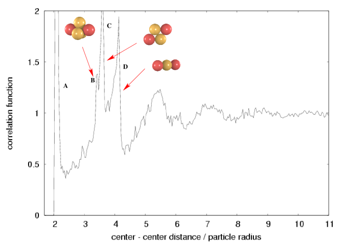
In Fig. 5 the particles cluster due to their attractive potentials and
form stable configurations. The diameter of the particles is m.
There is a sharp peak in the spacial correlation function of the particle centers at exactly
that distance , where two particles touch each other in the very left part of the plot (A). Then, for
larger particle separation, the correlation function starts to grow and drops suddenly after a peak at
(D), which is twice the diameter (). This is the contribution of two particles
touching the same third particle. The distance between them depends on the angle, which
they form with the particle in the middle, but, it is at last twice the diameter,
when they are in a straight line, which explains the sudden drop of the correlation function.
If several particles stick together, the straight line is stabilized. This explains the
peak at the end of this section of the correlation function.
Two more peaks can clearly be assigned
to configurations: One of them is from two particles touching two other particles, which themselves
touch each other (C). There again the case of all particles being in the same plane can be stabilized
by other particles surrounding them. The particles under consideration are then separated by a distance
of . But of course, bending this configuration is still a degree
of freedom which brings the two particles slightly closer to each other. Thus their contribution
to the correlation function is shifted downward.
The fourth peak at reflects two particles, both touching three particles,
which themselves are touching each other and define a plane (B). There is no freedom
anymore for the two particles touching all the three of them at the same time. One can place one
of them at one side of the plane and the other one at the other side.
When the potentials are mainly repulsive and the minimum caused by the van der Waals attraction
is only a fraction of , the spatial correlation function looks completely
different, as depicted in Fig. 6: The peaks described in the previous paragraphs
have disappeared here. The primary peak has moved to a slightly larger distance, since the
repulsive potential hinders the particles from touching each other.
In Fig. 7 we compare the correlation function of Fig. 6
with the potential used for that simulation. The maximum of the correlation function coincides
with the minimum of the potential, but, as the minimum is not very sharp, the particles are not
restricted to fixed geometries and are in a steady process of rearrangement which results in
broader peaks. This process could also be studied by evaluating the velocity correlation function
for the colloidal particles which is related to the viscosity of the sample.
The correlation of particles which are several diameters apart is still remarkable,
as it is transmitted by the particles in between.
The oscillations of the correlation function can be understood as a formation of layers where the
probability of finding a particle in a certain layer is higher than in between.

X.2 Shear
We have carried out simulations with shear and gravity. For the particles the boundaries in direction were closed, gravity was applied in negative -direction only to the colloidal particles. For the fluid particles the boundary in -direction was closed as well and additionally a velocity offset was added to apply a shear in -direction. Boundaries for fluid and for particles were periodic in - and -direction. Velocity distribution functions have been evaluated. For the cases we investigated, after a transient they are all Gaussian (Fig. 8).

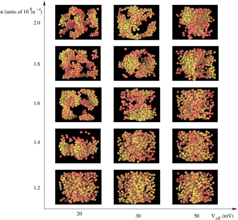
X.3 Phase diagram
We have explored the phase diagram for Al2O3 with respect to screening length and
effective surface potential. We could identify the regions of suspended single particles and
of flocculation (Fig. 9). The transition between these two regions
depends on both parameters, Debye screening length and effective surface potential.
It is known that the pH-value determines the effective surface potential ,
and that salt concentration and pH-value determine the Debye screening length Wang et al. (1999).
Exact relations between salt concentration and pH-value on one side and and
on the other side are not known a priori for the parameter ranges of our
suspensions. There are approximations for very diluted systems and low salt concentrations.
It is known that for Al2O3 the surface potential becomes zero for Hütter (1999).
However, a phase transition between clustering in the upper left part of Fig. 9
and a suspended regime in the lower right part can be found in the simulations in analogy to the
experiment. The spatial correlation function can be evaluated for all the simulated cases and it
can be used as a tool to identify the two regions of the phase diagram.
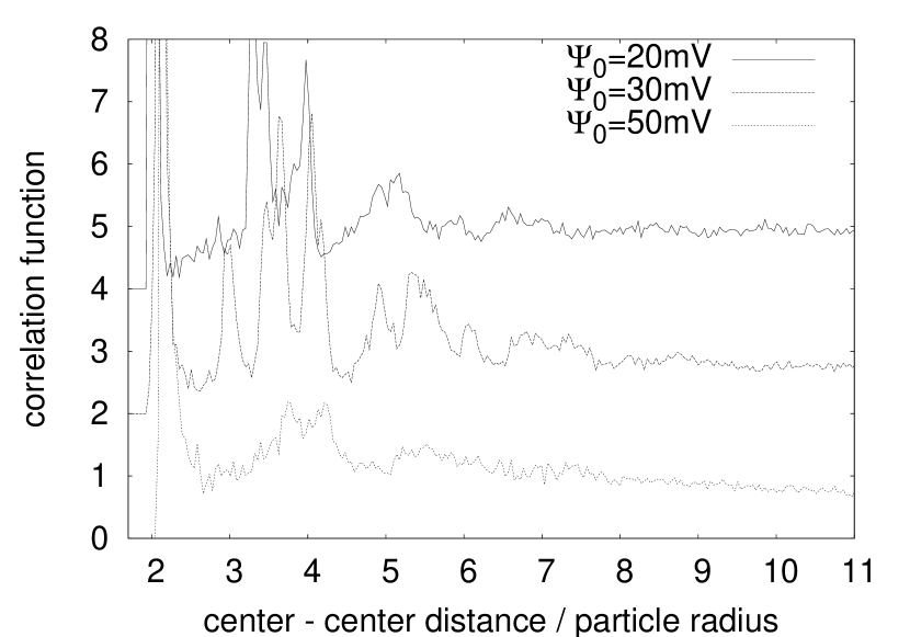
Figs. 10–13 show selected examples of correlation functions
for different parameter sets. The first and second graph refer to a volume fraction
which also has been used for the phase diagram of Fig. 9. In Fig. 10
the correlation function has been plotted for every other image of the left column in the phase diagram
in Fig. 9. One can see that for suspended particles only the first peak can be found
in the correlation function. The secondary minimum in the potential causes the particles to
glue for short times before they continue with their diffusion process. With increasing
the secondary minimum approaches the particle surface, and therefore the main peak is shifted
to smaller distances. At the same time it becomes deeper so that clusters are formed and more peaks
occur. The peak at a distance of disappears again, when the attraction becomes
stronger since this is a meta stable configuration of particles forming an octahedron.
Fig. 11 corresponds to the first row of images of Fig. 9.
In this case the depth of the secondary minimum is adjusted by changing the effective surface potential.
Again the transition between clustering regime and suspension can be observed. The potentials
used here are among the ones plotted above in Fig. 1444In current simulations
we did not yet distinguish between clustering in the primary or secondary minimum..
In Fig. 12 and 13 the dependence of the correlation function
on the volume fraction can be seen. In both cases long range correlations become more pronounced
with increasing volume fraction. This is shown for the suspended regime (Fig. 12)
and for the clustering regime (Fig. 13), where the transition between the two
cases presented here is achieved by a variation of by only .


X.4 Diffusion
We measured the diffusion coefficient of colloidal particles with attractive potentials. In Fig. 14 we show the diffusion coefficient for Al2O3 with an effective surface potential of and an inverse Debye screening length of for room temperature. One can see that the mobility of the particles decays since a cluster formation process takes place and the particles in the cluster are relatively fixed. The remaining mobility consists of two parts: Particles can still, with a non vanishing probability, leave the cluster by thermal activation and the cluster itself can take part in a diffusion process, it can vibrate or be deformed – all of these are processes which are taking place on much longer time scales than the single particle diffusion. By studying the dependency of the diffusion coefficient on the potentials and on the volume fraction, one might be able to find an answer to the question, which of these processes is important for the dynamics of the system in which part of the phase diagram of Fig. 9.
XI Conclusion
We have shown that by combining a Stochastic Rotation Dynamics and a Molecular Dynamics simulation
it is possible to study dense colloidal suspensions. We have explained how to determine effective
parameters for the simulation (box size , simulation time step ,
number of fluid particles per box …). It is possible to relate the simulation
to very distinct experimental conditions since all parameters (density, temperature,
potentials…) which enter into the description are scaled in a well defined manner.
We have presented first results which demonstrate the power of the model. We have demonstrated that
the Richardson-Zaki law is reproduced already with the simple and fast coupling method II and
we have studied the dependence of the pair correlation function on the shape of the interaction
potentials. We have shown how one can distinguish if for given Debye screening length ,
effective surface potential and Hamaker constant if the
system is in the clustering or suspended regime.
We are planning to carry out detailed investigations of the properties described in the two preceding
sections (diffusion coefficient, correlation functions, sedimentation velocity) as well
as cluster size and shape. Then these quantities can be analyzed under shear, their
dependence on the shear rate, and the shear viscosity of the suspension, containing the
fluid and the particles, which both contribute to a complex shear viscosity.

Acknowledgements.
This work has been financed by the German Research Foundation (DFG) within the project DFG-FOR 371 ”Peloide”. We thank G. Gudehus, G. Huber, M. Külzer, L. Harnau, J. Reinshagen, S. Richter, and M. Bier for valuable collaboration. We thank M. Strauss, A. Komnik, E. Tuzel, D. M. Kroll, A. J. Wagner, Y. Inoue and M. E. Cates for helpful discussions. T. Ihle thanks the SFB 404, project A7, of the DFG and ND EPSCoR through NSF grant EPS-0132289 for financial support.References
- Mahanty and Ninham (1996) J. Mahanty and B. W. Ninham, Dispersion Forces (Academic Press, London, 1996).
- Lagaly et al. (1997) G. Lagaly, O. Schulz, and R. Zimehl, Dispersionen und Emulsionen (Dr. Dietrich Steinkopff Verlag, Darmstadt, Germany, 1997).
- Shaw (1992) D. J. Shaw, Introduction to Colloid and Surface Chemistry (Butterworth-Heinemann Ltd, Oxford, 1992).
- Morrison and Ross (2002) I. D. Morrison and S. Ross, Colloidal Dispersions: Suspensions, Emulsions and Foams (John Wiley and Sons, New York, 2002).
- Schmitz (1993) K. S. Schmitz, Macroions in Solution and Colloidal Suspension (John Wiley and Sons, New York, 1993).
- Hunter (2001) R. J. Hunter, Foundations of colloid science (Oxford University Press, 2001).
- Richter and Huber (2003) S. Richter and G. Huber, Granular Matter 5, 121 (2003).
- Oberacker et al. (2001) R. Oberacker, J. Reinshagen, H. von Both, and M. J. Hoffmann, Ceramic Transactions 112, 179 (2001).
- Wang et al. (1999) G. Wang, P. Sarkar, and P. S. Nicholson, J. Am. Ceram. Soc. 82, 849 (1999).
- Lewis (2000) J. A. Lewis, J. Am. Ceram. Soc. 83, 2341 (2000).
- Hütter (2000) M. Hütter, Journal of Colloid and Interface Science 231, 337 (2000).
- Petera and Muthukumar (1999) D. Petera and M. Muthukumar, J. Chem. Phys 111, 7614 (1999).
- Ahlrichs et al. (2001) P. Ahlrichs, R. Everaers, and B. Dünweg, Phys. Rev. E 64, 040501 (2001).
- Ladd and Verberg (2001) A. J. C. Ladd and R. Verberg, J. Stat. Phys. 104, 1191 (2001).
- Adhikari et al. (2005) R. Adhikari, M. E. Cates, K. Stratford, and A. Wagner, condmat/0402598 (2005).
- Usta et al. (2005) O. B. Usta, A. Ladd, and J. Butler, J.Chem. Phys. 122, 094902 (2005).
- L.E. Silbert et al. (1997) L.E. Silbert, J.R. Melrose, and R.C. Ball, Phys. Rev. E 56, 7067 (1997).
- Malevanets and Kapral (1999) A. Malevanets and R. Kapral, J. Chem. Phys. 110, 8605 (1999).
- Malevanets and Kapral (2000) A. Malevanets and R. Kapral, J. Chem. Phys. 112, 7260 (2000).
- Padding and Louis (2004) J. T. Padding and A. A. Louis, Phys. Rev. Lett. 93, 220601 (2004).
- Noguchi and Gompper (2004) H. Noguchi and G. Gompper, Phys. Rev. Lett. 93, 258102 (2004).
- Ali et al. (2004) I. Ali, D. Marenduzzo, and J. Yeomans, J. Chem. Phys. 121, 8635 (2004).
- Tucci and Kapral (2004) K. Tucci and R. Kapral, The Journal of Chemical Physics 120, 8262 (2004).
- Russel et al. (1995) W. B. Russel, D. A. Saville, and W. Schowalter, Colloidal Dispersions (Cambridge Univ. Press., Cambridge, 1995).
- Schwarzer (1995) S. Schwarzer, Phys. Rev. E 52, 6461 (1995).
- Allen and Tildesley (1987) M. P. Allen and D. J. Tildesley, Computer simulation of liquids, Oxford Science Publications (Clarendon Press, 1987).
- Inoue et al. (2002) Y. Inoue, Y. Chen, and H. Ohashi, J. Stat. Phys. 107, 85 (2002).
- Ripoll et al. (2004) M. Ripoll, K. Mussawisade, R. G. Winkler, and G. Gompper, Europhys. Lett. 68, 106 (2004).
- Lamura et al. (2001) A. Lamura, G. Gompper, T. Ihle, and D. M. Kroll, Eur. Phys. Lett 56, 319 (2001).
- Ihle and Kroll (2001) T. Ihle and D. M. Kroll, Phys. Rev. E 63, 020201(R) (2001).
- Tuzel et al. (2003) E. Tuzel, M. Strauss, T. Ihle, and D. M. Kroll, Phys. Rev. E 68, 036701 (2003).
- Ihle and Kroll (2003a) T. Ihle and D. M. Kroll, Phys. Rev. E 67, 066705 (2003a).
- Ihle and Kroll (2003b) T. Ihle and D. M. Kroll, Phys. Rev. E 67, 066706 (2003b).
- Ihle et al. (2004) T. Ihle, E. Tuzel, and D. M. Kroll, Phys. Rev. E 70, 035701(R) (2004).
- Kikuchi et al. (2003) N. Kikuchi, C. M. Pooley, J. F. Ryder, and J. M. Yeomans, J. Chem. Phys. 119, 6388 (2003).
- Falck et al. (2004) E. Falck, J. M. Lahtinen, I. Vattulainen, and T. Ala-Nissila, Eur. Phys. J. E 13, 267 (2004).
- Winkler et al. (2004) R. G. Winkler, K. Mussawisade, M. Ripoll, and G. Gompper, J. of Physics-Condensed Matter 16 (2004).
- Blaak et al. (2004) R. Blaak, S. Auer, D. Frenkel, and H. Löwen, J. Phys.: Condens. Matter 16, S3873 (2004).
- Heyes (1983) D. M. Heyes, Chem. Phys. 82, 285 (1983).
- Richardson and Zaki (1954) J. F. Richardson and W. N. Zaki, Trans. Instn. Chem. Engrs. 32, 35 (1954).
- Hütter (1999) M. Hütter, Ph.D. thesis, Swiss Federal Institute of Technology Zurich (1999).