Spin current injection by intersubband transitions in quantum wells.

Abstract

We show that a pure spin current can be injected in quantum wells by the absorption of linearly polarized infrared radiation, leading to transitions between subbands. The magnitude and the direction of the spin current depend on the Dresselhaus and Rashba spin-orbit coupling constants and light frequency and, therefore, can be manipulated by changing the light frequency and/or applying an external bias across the quantum well. The injected spin current should be observable either as a voltage generated via the anomalous spin-Hall effect, or by spatially resolved pump-probe optical spectroscopy.

Spin current is an interesting physical phenomenon in its own right, and could have application in the delivery and transfer of electron spins in spintronics devices. From a fundamental point of view, various issues raised in the theory of this effect are far from being satisfactorily settled. As was shown by Rashba Rashba03 , a spin current exists even in the equilibrium state of a two-dimensional (2D) electron gas with spin-orbit (SO) coupling. The application of an external electric field has been suggested as a strategy for driving the system out of equilibrium and inducing a spin current exhibiting transport effects. Mal’shukov et al. Malshukov03 and Governale et al. Governale03 suggested applying a time-dependent bias across a semiconducting heterostructure, thus modulating the strength of the SO coupling and generating a spin current. Murakami et al. Murakami03 and Sinova et al. Sinova04 have shown that an in-plane electric field can cause a spin current, leading to the ”intrinsic spin-Hall effect”. Another possibility for the injection of spin current is coherently controlled optical excitations between the valence and the conduction band, as predicted by Bhat and Sipe Bhat00 ; Bhat04 and observed experimentally in bulk crystals Stevens02 ; Hubner03 and quantum wells (QWs) Stevens03 .

Here we show that a spin current can be injected in QWs by infrared (IR) light absorption, driving transitions between different subbands. The injection of spin-polarized electric current in QWs due to intersubband transitions caused by circularly polarized radiation has already been observed by Ganichev et al. Ganichev03 . In contrast, here we investigate a pure spin current, where electrons moving in opposite directions have opposite orientations of spins, not accompanied by a net electrical current. We show that the strength and direction of this pure spin current can be manipulated by modulating the SO coupling strength via applied bias Nitta97 and/or adjusting the light frequency.

As an example we consider the (011) GaAs QW, where the electron spins have a considerable out-of plane component, thus making possible the observation of the pure spin current by detecting the voltage generated via the anomalous spin-Hall effect Abakumov72 ; Bakun85 . The first two subbands in the well are typically separated by the energy $\hbar\omega_{0}\approx 100$ meV; the exact value depends on the width of the QW, dopant concentration, and the boundary conditions. The SO Hamiltonian for the (011) QW, ${H}_{\mathrm{SO}}={H}_{D}+{H}_{R},$ is the sum of a Dresselhaus term Dyakonov86 , ${H}_{D},$ originating from the unit cell inversion asymmetry, and a Rashba term Rashba84 , ${H}_{R},$ originating from the asymmetric doping and/or a bias applied across the well:

$${H}_{D}^{[n]}=\alpha_{D}^{[n]}k_{y}{\sigma}^{{}_{z}}F_{[n]}(\mathbf{k)},\qquad{H}_{R}^{[n]}=\alpha_{R}^{[n]}\left({\sigma}^{x}k_{y}-{\sigma}^{y}k_{x}\right),$$ (1)

where $n$ is the subband index, $\mathbf{k}=(k_{x},k_{y})$ is the in-plane wavevector of the electron envelope function, $F_{[n]}(\mathbf{k)=}1-\left(k_{y}^{2}-2k_{x}^{2}\right)\lambda_{[n]}^{2}$, where $\lambda_{[n]}$ depends on the QW width $w$, and the ${\sigma}^{i}$ are the Pauli matrices. The $z-$axis is perpendicular to the QW plane and the in-plane axes are: $x=[100]$ and $y=[0\overline{1}1]$. The parameters $\alpha_{D}^{[n]}$ and $\alpha_{R}^{[n]}$ depend on $n$; in the model of rigid QW walls one has $\alpha_{D}^{[n]}=-\alpha_{0}n^{2}\left(\pi/w\right)^{2}/2$, where $\alpha_{0}$ is the Dresselhaus constant for the bulk, and $\lambda_{[n]}=w/n\pi$ Dyakonov86 . The deviation of $F_{[n]}(\mathbf{k)}$ from unity becomes important at electron concentrations $N_{\mathrm{el}}\approx 10^{12}$ cm^-2.

The spin-related energy is given by $E_{\mathrm{SO}}^{[n]}\left(\mathbf{k}\right)=\sqrt{\left(\alpha_{D}^{[n]}k_{y}F_{[n]}(\mathbf{k)}\right)^{2}+\left(\alpha_{R}^{[n]}k\right)^{2}},$ with ”up” $(u)$ and ”down” $(d)$ states having energies $E_{u,d}^{[n]}\left(\mathbf{k}\right)=\pm E_{\mathrm{SO}}^{[n]}\left(\mathbf{k}\right)$, and leads to the subband spectra:

$$\varepsilon_{s_{1}}=\frac{\hbar^{2}k^{2}}{2m}\pm E_{\mathrm{SO}}^{[1]}\left(\mathbf{k}\right),\qquad\varepsilon_{s_{2}}=\hbar\omega_{0}+\frac{\hbar^{2}k^{2}}{2m}\pm E_{\mathrm{SO}}^{[2]}\left(\mathbf{k}\right).$$ (2)

where $m$ is the electron effective mass and the indices $s_{1},s_{2}$ describe the $u(+)$ and $d(-)$ spin states in the subbands $n=1$ and $n=2$, respectively. The corresponding spin eigenstates $\phi^{s_{n}}_{\bf k}$ result in expectation values of the spin components:

$$\langle\left.\phi^{s_{n}}_{\bf k}\right|\sigma^{z}\left|\phi^{s_{n}}_{\bf k}\right.\rangle=\pm\frac{\alpha_{D}^{[n]}k_{y}F_{[n]}(\mathbf{k)}}{E_{\mathrm{SO}}^{[n]}\left(\mathbf{k}\right)},\qquad\langle\left.\phi^{s_{n}}_{\bf k}\right|{\sigma}_{\|}\left|\phi^{s_{n}}_{\bf k}\right.\rangle=\pm\frac{\alpha_{R}^{[n]}}{E_{\mathrm{SO}}^{[n]}\left(\mathbf{k}\right)}(k_{y},-k_{x}),$$ (3)

where upper(lower) sign corresponds to the $u(d)$ state and $\mathbf{\sigma}_{\|}=(\sigma^{x},\sigma^{y})$.

There is not yet consensus in the literature on the fundamental description of spin current, and the effect of disorder on it, as discussed e.g., in Ref.SHE ; spin current is not a ”true” current, in that its density does not satisfy a continuity equation describing the evolution of a spin density Rashba03 . Nonetheless, we introduce a ”physical” definition of spin current per electron as:

$$j_{\mu}^{\beta}\left(\mathbf{k,}s_{n}\right)=\frac{\hbar}{4}\cdot\langle\left.\phi^{s_{n}}_{\bf k}\right|v_{\mu}{\sigma}^{\beta}+{\sigma}^{\beta}v_{\mu}\left|\phi^{s_{n}}_{\bf k}\right.\rangle,$$ (4)

where $\mu$ and $\beta$ are Cartesian indices. Velocity components ${v}_{i}=\partial{H}/\hbar\partial k_{i}$ are the sums of normal ${v}_{i,{\rm n}}=\hbar k_{i}/m$ and anomalous terms given in our model (Eq.(1)) by:

$$v_{x,{\rm an}}^{[n]}=-\frac{\alpha_{R}^{[n]}}{\hbar}{\sigma}^{y}+4k_{y}k_{x}\frac{\alpha_{D}^{[n]}}{\hbar}{\sigma}^{z}\lambda_{[n]}^{2},\qquad v_{y,{\rm an}}^{[n]}=\frac{\alpha_{D}^{[n]}}{\hbar}\left(1-\left(3k_{y}^{2}-2k_{x}^{2}\right)\lambda_{[n]}^{2}\right){\sigma}^{z}.$$ (5)

Below we consider only the spin current components associated with the $z-$axis spin projection. First we calculate the equilibrium spin current at typical experimental conditions, where only the first subband is occupied, and then find the changes induced by the intersubband excitations. For this purpose we introduce the equilibrium Fermi distribution function for two spin projections in the first subband:

$$f_{\pm}(\mathbf{k})=\frac{1}{\exp\left[\left(\hbar^{2}k^{2}/2m\pm E^{[1]}_{\mathrm{SO}}(\mathbf{k})-\mu\right)/k_{B}T\right]+1},$$ (6)

where $\mu$ is the chemical potential for a given $N_{\mathrm{el}}$, and $k_{B}$ is the Boltzmann’s constant. The spin current density component $J_{y}^{z}$ is the sum of the normal, $J_{y,{\rm n}}^{z}$, and the anomalous, $J_{y,{\rm an}}^{z}$, parts. By integrating $j_{\mu}^{\beta}\left(\mathbf{k,}s_{1}\right)$ over the equilibrium state we obtain:

$$J_{y}^{z}=\frac{\hbar}{2}\left\{\frac{\alpha_{D}^{[1]}}{\hbar}\int\left(f_{+}\left(\mathbf{k}\right)+f_{-}\left(\mathbf{k}\right)\right)\left(1-\left(3k_{y}^{2}-2k_{x}^{2}\right)\lambda_{1}^{2}\right)\frac{d^{2}k}{\left(2\pi\right)^{2}}+\frac{\hbar}{m}\int\left(f_{+}\left(\mathbf{k}\right)-f_{-}\left(\mathbf{k}\right)\right)k_{y}\left.\langle\phi^{u_{1}}_{\bf k}\right|\sigma^{z}\left|\phi^{u_{1}}_{\bf k}\right.\rangle\frac{d^{2}k}{\left(2\pi\right)^{2}}\right\},$$ (7)

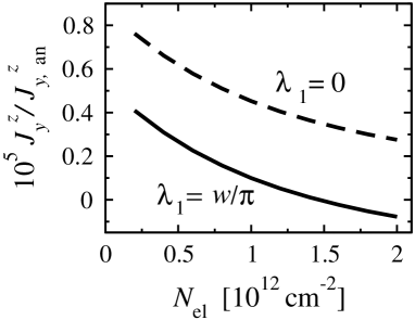
Figure 1: Spin current $J_{y}^{z}/J_{y,\mathrm{an}}^{z}$ as a function of the electron concentration $N_{\mathrm{el}}$. Dashed curve : $\lambda_{1}=0$, solid curve $\lambda_{1}=w/\pi$, the QW width $w=80$ Å. The parameters are: $\alpha_{D}^{[1]}$=-0.3$\times 10^{-9}$ eVcm, $\alpha_{R}^{[1]}$=-0.3$\alpha_{D}^{[1]}$, $k_{B}T$=25 meV, $m=0.066m_{0},$ where $m_{0}$ is a free electron mass.

where $\left.\langle\phi^{u_{1}}_{\bf k}\right|\sigma^{z}\left|\phi^{u_{1}}_{\bf k}\right.\rangle$ is defined in Eq.(3), and $J_{x}^{z}=0$ by symmetry. The contributions $J_{y,{\rm an}}^{z}$ and $J_{y,{\rm n}}^{z}$ (first and second term in Eq.(7), respectively) almost cancel each other. At $T=0$ each of them is close in absolute value to $\left|\alpha_{D}^{[1]}\right|N_{\mathrm{el}}/2\left(1-\pi N_{\mathrm{el}}\lambda_{[n]}^{2}/2\right)$, and $J_{y}^{z}/J_{y,\mathrm{an}}^{z}\approx\left(m\alpha_{R}^{[1]}/\hbar^{2}k_{F}\right)^{2}\ll 1$ where $\hbar k_{F}$ is the Fermi momentum (see also Rashba Rashba03 ). We show $J_{y}^{z}/J_{y,\mathrm{an}}^{z}$ as a function of $N_{\rm el}$ in Fig. 1.

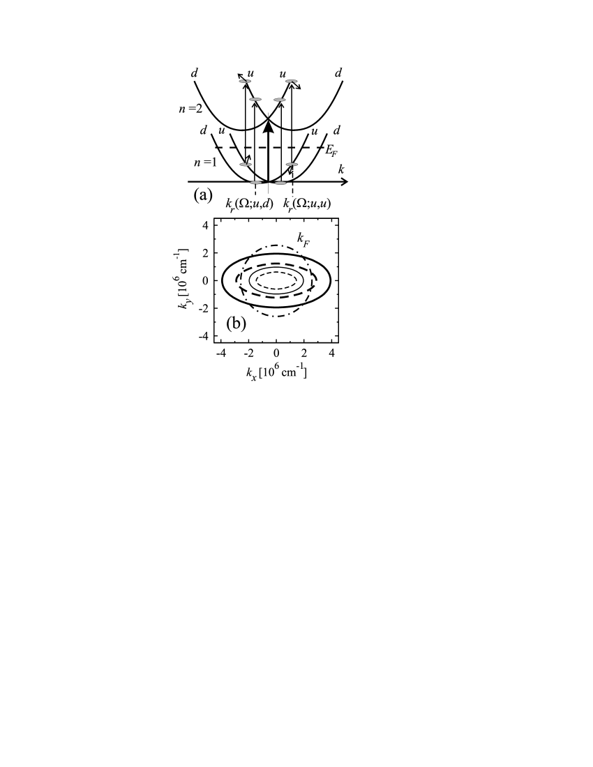
Figure 2: (a) The intersubband transitions leading to the injection of pure spin current. Thick arrow line corresponds to $\Omega=0$. Thin arrow lines correspond to transitions at $\Omega>0$. (b) Resonance curves $\mathbf{k}=\mathbf{k}_{r}^{s_{2},s_{1}}(\Omega)$. Solid (dash) lines describe the spin-conserving (spin-flip) transitions. In each case the outer curve is for $\hbar\Omega=2$ meV and the inner curve for $\hbar\Omega=1$ meV. The circle marked as $k_{F}$ is the Fermi line at $N_{\rm el}=10^{12}$ cm^-2. The parameters are: $\alpha_{D}^{[1]}$=-0.3$\times 10^{-9}$ eVcm, $\alpha_{R}^{[1]}$=-0.3$\alpha_{D}^{[1]}$, $\alpha_{D}^{[2]}$=4$\alpha_{D}^{[1]}$, $\alpha_{R}^{[2]}$=-0.5$\alpha_{D}^{[2]}$, and $\lambda_{[n]}=w/n\pi$.

Now we can investigate the spin current injection by linearly-polarized IR radiation due to the intersubband transitions, as shown in Fig. 2a. The external field is a pulse $\mathbf{E}(t)=\mathcal{E}(t)\exp\left(-i\omega t\right)+c.c.$ with the carrier frequency $\omega$, and slowly varying amplitude $\mathcal{E}(t)$ of duration $\tau$. We consider oblique incidence with $\mathcal{E}(t)$ lying in the plane of incidence. The radiation frequency $\omega$ is close to $\omega_{0}$, with a detuning $\Omega=\omega-\omega_{0}$, such that it can cause transitions between the subbands, with $\hbar\Omega$ being of the order of few meV. For $\tau\gg\omega^{-1}$ the exact shape of the pulse has no influence on our results; however, to have the possibility of momentum-selective excitations as shown in Fig.2a one needs sufficiently long pulses, with $\tau>\hbar/\alpha_{D}k_{F}\approx 1$ ps, for $\alpha_{D}$ $\approx 10^{-9}$ eV$\cdot$cm, a typical value of the Dresselhaus coupling Dyakonov86 . This condition also implies applicability of Fermi’s Golden Rule, since the pulse contains many periods of the field oscillations. Since $\alpha_{D}^{[n]},$ $\alpha_{R}^{[n]}$ and, in turn, the spin states and anomalous velocities depend on the subband, the intersubband transitions can cause the injection of a spin current. The ratio $\alpha_{D}^{[n]}F_{[n]}(\mathbf{k})/\alpha_{R}^{[n]}$, which determines the direction of the effective SO field acting on the spin, depends on the subband. Therefore, the spin states in different subbands are not mutually orthogonal, so $\left.\langle\phi^{s_{1}}_{\bf k}\right|\phi^{s_{2}}_{\bf k}\rangle\neq 0$, and, ”spin-flip” transitions $u\longleftrightarrow d$ are allowed with linearly polarized IR light absorption. The transitions $\phi^{s_{1}}_{\bf k}\rightarrow\phi^{s_{2}}_{\bf k}$ occur in the vicinity of the resonance curves in the momentum space, determined by the $\mathbf{k}=\mathbf{k}_{r}^{s_{2},s_{1}}(\Omega)$ where $\mathbf{k}_{r}^{s_{2},s_{1}}(\Omega)$ is specified by the constraint of energy conservation. For a given $\Omega$ there are in fact two such curves. In our case $E_{\mathrm{SO}}^{[2]}\left(\mathbf{k}\right)>E_{\mathrm{SO}}^{[1]}\left(\mathbf{k}\right)$ for all $k$. Therefore, for $\Omega>0$ the transitions $d\rightarrow u$ and $u\rightarrow u$ are allowed, while for $\Omega<0$ we obtain $d\rightarrow d$ and $u\rightarrow d$ transitions. As one can see in Figs. 2a and 2b, $k_{r}^{s_{2},s_{1}}(\Omega)$ is larger for the ”spin-conserving” than for the ”spin-flip”-transitions.

The transition matrix elements depend on the spin states in both subbands, and can be factorized in the dipole approximation as:

$$M\left(\mathbf{k}_{r}^{s_{2},s_{1}}(\Omega)\right)=\mathcal{E}e\frac{\sin 2\theta_{0}}{\epsilon\cos\theta_{0}+\sqrt{\epsilon}\cos\theta_{1}}\left\langle\varphi^{(2)}(z)\right|z\left|\varphi^{(1)}(z)\right\rangle\left\langle\phi^{s_{2}}_{\bf k}\right|\left.\phi^{s_{1}}_{\bf k}\right\rangle,\qquad$$ (8)

where $\theta_{0}$ and $\theta_{1}$ are, respectively, the incidence and refraction angles, $\sin\theta_{1}=\sin\theta_{0}/\sqrt{\epsilon}$, $\epsilon$ is the dielectric constant, $e$ is the electron charge, and $\varphi^{(1)}(z)$, $\varphi^{(2)}(z)$ are the envelope electron wavefunctions in the subbands $n=1$ and $n=2,$ respectively. A transfer of one electron to the second subband injects a spin current:

$$\Delta j_{y}^{z}\left(\mathbf{k;}s_{2},s_{1}\right)=j_{y}^{z}\left(\mathbf{k,}s_{2}\right)-j_{y}^{z}\left(\mathbf{k,}s_{1}\right),$$ (9)

where we neglect the small photon momentum. The incident radiation injects the concentration of electrons in the second subband $N_{2}$, with a rate $dN_{2}\left(\Omega\right)/dt$ and, correspondingly, drives the spin current density component with the rate $d\Delta J_{y}^{z}\left(\Omega\right)/dt.$ The injection rates can be written as:

$$\frac{d\Delta J_{y}^{z}\left(\Omega\right)}{dt}=\frac{\hbar}{2}\zeta(\Omega)\frac{dN_{2}\left(\Omega\right)}{dt},\qquad\frac{dN_{2}\left(\Omega\right)}{dt}=\frac{\xi(\Omega)}{\hbar\omega}\left\langle S\right\rangle,$$ (10)

where $\zeta(\Omega)$ characterizes the effective speed of electrons forming the pure spin current, $\left\langle S\right\rangle=(c/2\pi)\mathcal{E}^{2}$ is the radiation power per unit area, and $\xi(\Omega)$ is a dimensionless function.

Within Fermi’s Golden Rule the speed characterizing the spin injection is obtained as:

$$\frac{\hbar}{2}\zeta(\Omega)=\frac{\sum\limits_{s_{1},s_{2}}\displaystyle{\int}f_{s_{1}}\left(\mathbf{k}\right)\left|\langle\phi_{\bf k}^{s_{2}}\right|\left.\phi_{\bf k}^{s_{1}}\rangle\right|^{2}\Delta j_{y}^{z}\left(\mathbf{k;}s_{2},s_{1}\right)dk_{r}^{s_{2},s_{1}}(\Omega)/v^{s_{2},s_{1}}_{\mathbf{k}}}{\sum\limits_{s_{1},s_{2}}\displaystyle{\int}f_{s_{1}}\left(\mathbf{k}\right)\left|\langle\phi_{\bf k}^{s_{2}}\right|\left.\phi_{\bf k}^{s_{1}}\rangle\right|^{2}dk_{r}^{s_{2},s_{1}}(\Omega)/v^{s_{2},s_{1}}_{\mathbf{k}}},$$ (11)

with the velocity associated with the joint density of states given by:

$$\mathbf{v}^{s_{2},s_{1}}_{\mathbf{k}}=\frac{\partial}{\hbar\partial\mathbf{k}}\left(\varepsilon_{s_{2}}-\varepsilon_{s_{1}}\right).$$ (12)

The integration in Eq.(11) is performed along the resonance curves. With the increase of $\left|\Omega\right|$, $k_{r}^{s_{2},s_{1}}(\Omega)$ increases and eventually arrives at regions of small electron occupancy, as can be seen in Fig. 2b. Hence, $d\Delta J_{y}^{z}\left(\Omega\right)/dt$ and $dN_{2}/dt$ become small at $\hbar\left|\Omega\right|$ larger than some critical $\hbar\Omega_{\rm c}$ (a few meV) determined by the condition $\min k_{r}^{s_{2},s_{1}}(\Omega_{\rm c})>k_{0}$, where $k_{0}=k_{F}$ or $k_{0}=\sqrt{mk_{B}T}/\hbar$ in the degenerate and non-degenerate gas, respectively.

The photoinduced spin current is the sum of normal $\Delta J_{y,\mathrm{n}}^{z}$ and anomalous $\Delta J_{y,\mathrm{an}}^{z}$ contributions, each containing spin-flip $\left(s_{1}\neq s_{2}\right)$ and spin conserving $\left(s_{1}=s_{2}\right)$ terms. The anomalous spin-conserving term is of the order of $\left(\alpha_{D}^{[2]}-\alpha_{D}^{[1]}\right)N_{2},$ while the other terms depend on the difference of the ratio $\alpha_{R}^{[2]}/\alpha_{D}^{[2]}-\alpha_{R}^{[1]}/\alpha_{D}^{[1]}$ and $\lambda_{[n]}$. An estimate of the relative contributions is:

$$\frac{\Delta J_{y,\mathrm{n}}^{z}\left(s_{1}=s_{2}\right)}{\Delta J_{y,\mathrm{an}}^{z}\left(s_{1}=s_{2}\right)}\approx\frac{\hbar^{2}k_{F}}{m\alpha_{D}}\left[\left(\frac{\alpha_{R}^{[2]}}{\alpha_{D}^{[2]}}\right)^{2}-\left(\frac{\alpha_{R}^{[1]}}{\alpha_{D}^{[1]}}\right)^{2}\right].$$ (13)

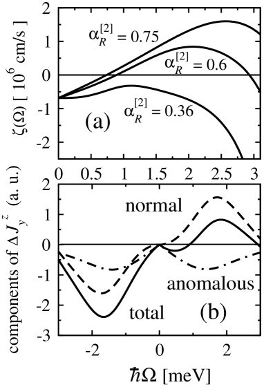
Figure 3: (a) The speed $\zeta(\Omega)$ for different Rashba coupling constants $\alpha_{R}^{[2]}$ (values in 10^-9 eVcm units are presented near the curves). Other parameters are the same as in Fig.2, $N_{\mathrm{el}}=10^{12}$ cm^-2, and $k_{B}T$=25 meV. The direction of the spin current can be altered by changing the Rashba parameter. (b) Components of the induced spin current as the function of the photon frequency for $\alpha_{R}^{[2]}=0.6\times 10^{-9}$ eVcm.

Due to a large prefactor $\hbar^{2}k_{F}/m\alpha_{D},$ which is the ratio of the normal and anomalous velocities, the normal term can be large and lead to a change in the sign of the spin current at particular light frequencies, as seen in Figs.3a and 3b. In Fig.3a we present the speed $\zeta(\Omega)$, while in Fig.3b we show the normal and anomalous parts of the injected spin current density. The spin-flip contribution in both the normal and anomalous terms is much smaller than the ”spin-conserving” one. Recently, Golub Golub03 demonstrated that the direction of electric current induced by interband light absorption in QWs can depend on the light frequency. In his scenario the change occurs as new subbands are accessed, and thus appears on a scale of 100 meV. In our scenario for pure spin current injection, the change occurs on a much smaller scale.

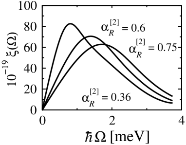
Figure 4: $\Omega$-dependence of $\xi(\Omega)$ for different Rashba parameters $\alpha_{R}^{[2]}$. The units of incident light power density are $\mathrm{W/cm}^{2}$. We take an incidence angle $\theta_{0}=\pi/4$, $\epsilon=12$, and $w=80$ Å. The infinite barrier approximation is used for the calculation.

Now we estimate the magnitude of the injected spin current assuming that the contributions of the anomalous and normal terms are of the same order of magnitude. Fig.4 presents the efficiency of the energy absorption $\xi(\Omega)$ (Eq.(10)). The concentration of the electrons excited to the second subband can be estimated from Eqs.(8)-(10) as $N_{2}\approx 2\pi(e^{2}w^{2}k_{F}/\epsilon^{2}\hbar c\alpha_{D})\langle S\rangle\tau$. At $\epsilon=12$, $k_{F}\approx 10^{6}$ cm${}^{-1},w=100$ Å, $\theta_{0}$ close to $\pi/4$ and $N_{\mathrm{el}}\approx 10^{12}$ cm^-2 we obtain: $N_{2}/N_{\mathrm{el}}\approx 10^{-6}$ $\left(\langle S\rangle/(\mathrm{W/cm}^{2})\right)\cdot\left(\tau/\mathrm{ps}\right)$. Under excitation of a 1% fraction of electrons, achieved at $\langle S\rangle\approx 10$ $\mathrm{kW/cm}^{2}$ and $\tau\approx 1$ $\mathrm{ps,}$ the corresponding effective current density $e\Delta J_{y}^{z}/\hbar\approx 1$ $\mathrm{mAmp/cm.}$ This is of the same magnitude as would be generated by the ac spin pumping in the $n=1$ subband, as proposed by Mal’shukov et al. Malshukov03 , but the effect would operate on a nanosecond time scale, as opposed to the picosecond time scale relevant here.

Having found the magnitude of the spin current, we discuss its experimental observation. A possible technique is the measurement of the voltage generated by the anomalous spin-Hall effect due to scattering of electrons by impurities. The spin current $\Delta J_{y}^{z}$ causes a spin-Hall bias $V_{sH}$ along the $x$ axis. Its magnitude can be estimated as $V_{sH}\approx\tan(\theta_{sH})V_{\mathrm{eff}}$, where $\theta_{sH}$ is the spin-Hall angle and $V_{\mathrm{eff}}$ is the effective lateral bias that would cause a current density $e\Delta J_{y}^{z}/\hbar$. As follows from the discussion preceding Eq.(13), the corresponding current density is of the order of $eN_{2}(\alpha_{D}/\hbar)$. The bias $V_{\mathrm{eff}}$ that would cause this current density is: $V_{\mathrm{eff}}\approx L\left(N_{2}/N_{\mathrm{el}}\right)\alpha_{D}/\hbar\mu$, where $\mu$ is the mobility, and $L\approx 1$ cm is the lateral size of the system. At $\mu\approx 10^{5}$ $\mathrm{cm}^{2}/(\mathrm{Vs})$, $N_{2}/N_{\mathrm{el}}\approx 10^{-3}$, and $\alpha_{D}/\hbar\approx 10^{6}$ cm/s we obtain: $V_{\mathrm{eff}}/L\approx 10^{-2}$ $\mathrm{V/cm.}$ The spin-Hall angle was estimated by Huang et al. Huang04 as $\theta_{sH}\approx 10^{-3}$, which would lead to $V_{sH}\approx 10^{-5}$ V. Their model assumed charged dopants embedded directly in the QW, which considerably overestimates the magnitude of the effect when only a remote doping is present. For this reason, $10^{-5}$ V is clearly an upper estimate of the spin Hall bias. Nonetheless, even a bias smaller by two orders of magnitude than this would be experimentally accessible Bakun85 .

Another possibility for observing the pure spin current is spatially resolved pump-probe spectroscopy, as applied by Hübner et al. Hubner03 and Stevens et al. Stevens03 to investigate the spin current injected by interband transitions. In those experiments the centers of the spin-up and spin-down of excited electron distribution were separated by approximately 20 nm. In the experimental situation considered here, the spin-polarized spots can be separated by distances of the order of the electron free path $\ell\approx\left(\hbar k_{F}/m\right)\tau_{k},$ with $\tau_{k}$ being the momentum relaxation time. At mobility $\mu\approx 10^{5}$ $\mathrm{cm}^{2}/(\mathrm{Vs}),$ one obtains $\ell\approx 10^{3}$ nm, and so a possible approach would be to observe this separation experimentally by using a linearly polarized IR light as a pump and circularly polarized light as a probe of the spin-dependent transmission. In a real sample, of course, we have to expect some inhomogeneity in the spin-orbit interaction due to quantum well thickness variations, dopant fluctuations, inhomogeneous strain, and the like Sherman03 . We are currently investigating the consequences of such inhomogeneity, and will return to it in a later communication.

To conclude, we have shown that a pure spin current can be injected in QWs by IR intersubband absorption, calculated its magnitude, and found that it could be measured experimentally. The dependence of the spin current on the light frequency, and on the Rashba SO coupling parameter, opens the possibility of its manipulation applying an external bias and by changing the light frequency. The spin current should be observable by anomalous spin-Hall effect measurements or by pump-probe optical spectroscopy.

E.Y.S is grateful to the Austrian Science Fund for financial support. A.N. acknowledges support from an Ontario Graduate Scholarship. This work was supported in part by the National Science and Engineering Research Council or Canada (NSERC) and the DARPA SpinS program. We thank P. Marsden, H. van Driel, and J. Sinova for useful discussions.

References

(1) E.I. Rashba, Phys. Rev. B 68, 241315 (2003).
(2) A. G. Mal’shukov, C. S. Tang, C. S. Chu, and K. A.Chao,
Phys. Rev. B 68, 233307 (2003).
(3) M. Governale, F. Taddei, and R. Fazio,
Phys. Rev. B 68, 155324 (2003).
(4) S. Murakami, N. Nagaosa, and S.-C. Zhang,
Science 301, 1348 (2003).
(5) J. Sinova, D. Culcer, Q. Niu, N. A. Sinitsyn,
T. Jungwirth, and A. H. MacDonald,
Phys. Rev. Lett. 92, 126603 (2004).
(6) R. D. R. Bhat and J. E. Sipe, Phys.
Rev. Lett.85, 5432 (2000).
(7) R. D. R. Bhat, F. Nastos, Ali Najmaie, and J. E. Sipe,
preprint cond-mat/0404066 (unpublished)
(8) M. J. Stevens, A. L. Smirl, R. D. R. Bhat,
J. E. Sipe, and H. M. van Driel,
J. Appl. Phys. 91, 4382 (2002).
(9) J. Hübner, W.W. Rühle, M. Klude, D. Hommel,
R.D.R. Bhat, J.E. Sipe, and H.M van Driel,
Phys. Rev. Lett. 90, 216601 (2003).
(10) M. J. Stevens, A. L. Smirl, R. D. R. Bhat, A. Najmaie,
J. E. Sipe, and H. M. van Driel, Phys. Rev. Lett. 90, 136603 (2003).
(11) S. D. Ganichev, P. Schneider, V. V. Bel’kov, E. L.
Ivchenko, S. A. Tarasenko, W. Wegscheider, D. Weiss, D. Schuh, B. N. Murdin,
P. J. Phillips, C. R. Pidgeon, D. G. Clarke, M. Merrick, P. Murzyn, E. V.
Beregulin, and W. Prettl, Phys. Rev. B 68, 081302(R) (2003). For a
review, see S. D. Ganichev and W. Prettl, J. Phys.: Condens. Matter, 15 R935 (2003).
(12) J. Nitta, T. Akazaki, H. Takayanagi, and T. Enoki, Phys.
Rev. Lett. 78, 1335 (1997).
(13) V.N. Abakumov and I.N. Yassievich,
Sov. Phys. JETPh 34, 1375 (1972),
P. Nozieres and C. Lewiner,
Journal de Physique, 10, 901 (1973).
(14) A.A. Bakun, B.P. Zakharchenya, A.A. Rogachev, M.N.
Tkachuk, and V.G. Fleisher, JETP Lett. 40, 1293 (1984)
(15) M.I. Dyakonov and Y.Yu. Kachorovskii, Sov. Phys.
Semicond. 20, 110 (1986). For holes, see: E.I. Rashba and E.Ya. Sherman, Phys. Lett.
A 129, 175 (1988).
(16) Yu. A. Bychkov and E. I. Rashba, JETP Lett. 39,
79 (1984), E.I. Rashba, Sov. Phys. - Solid State 2, 1874, (1964).
(17) K. Nomura, J. Sinova, T. Jungwirth, Q. Niu, and A. H. MacDonald,
Phys. Rev. B 71, 041304(R) (2005),
L. Sheng, D. N. Sheng, and C. S. Ting,
Phys. Rev. Lett. 94, 016602 (2005).
(18) L.E. Golub, Phys. Rev. B 67, 235320 (2003).
(19) H. C. Huang, O. Voskoboynikov, and C. P. Lee, J. Appl.
Phys. 95, 1918 (2004).
(20) E.Ya. Sherman,
Appl. Phys. Lett. 82, 209 (2003),
L. E. Golub and E. L. Ivchenko,
Phys. Rev. B 69, 115333 (2004).