Spin Polarization and Dichroism Effects by Electric Field

Abstract

We show that electric field can induce spin polarization and dichroism effects in angle resolved photoemission spectroscopy (ARPES) in spin orbit coupling systems. The physical origin behind the effects essentially is the same as the spin Hall effect induced by the electric field. Since the ARPES experiments have both energy and momentum resolutions, the spin Hall effect can be directly verified by the ARPES experiments for individual band even if there is no net spin current.

The field of spintronics, which manipulate the spin degree of freedom in solid state devices, has been an active field of research. One important research in this field is to create, control and detect spin current. Recently, a new spin current source has been suggestedMurakami2003 ; Sinova2004 . It is proposed theoretically that a spin Hall current can be generated in strongly spin-orbit coupling systems by external electric field. The spin Hall effect exists in a broader class of spin-orbit coupling models. It has been evolved into a subject of intense theoretical researchHu2003 ; Bernevig2004a ; Culcer2004a ; Rashba2003 ; Murakami2004a ; Murakami2004b ; Murakami2004c ; Rashba2004 ; Bernevig2004b ; Burkov2004a ; Chang2004 ; Hirsch2004 ; Schliemann2003 ; Schliemann2004a ; Sinitsyn2004a ; Shen2004a ; Sheng2004b ; Liu2004 .

The spin Hall effect can be easily derived from the single particle quantum mechanics. In real materials, due to disorder, theoretically it is still controversial whether the effect exists or not. Recently, two experimental groups Kato2004 ; Wunderlich2004 have reported that the spin Hall effect has been observed in two dimensional hole systems with Rashba spin-orbit coupling, which contradicts the theoretical analysis in the presence of disorderMishchenko2004 ; Ioue2004 . Therefore, independent experiment is still required to verify the effect.

In this paper, we propose that angle resolved photoemission spectroscopy(ARPES) can be used to detect the spin Hall effect in spin-orbit coupling systems. We show that electric field can induce spin polarization and dichroism effects in angle resolved photoemission spectroscopy (ARPES) in spin orbit coupling systems without any magnetization. The effects stem from the same physical origins as the spin Hall effect. The ARPES is a very powerful tool to study condensed matter materials, such as cupratesDamascelli2003 . Compared to other experimental techniques, there are several advantages. First, the ARPES experiments have both energy and momentum resolutions which provide the detailed electronic physics of individual band. In particular, we will show that it is not required to have spin current flowing in samples in order to verify the spin Hall effect. Therefore, there could be no magnetization at the edges of samples. The signal is induced purely by electric field. Secondly, the ARPES has been used to measure the spin-orbit couplingMizokawa2001 ; Rotenberg1999 . The experimental setup discussed here is straightforward. Finally, there are several independent quantities which can be measured to test the physics of the spin Hall effect.

Before discussing ARPES measurements, let’s consider the original physics of the spin Hall effect. The result that we want to emphasize is that, in general, there is dissipationless spin Hall current in each band in spin-orbit coupling systems even if the total net spin Hall current is zero. Imagining two bands which is split by the spin-orbit coupling from a spin-degenerated band, there is no net spin current created by external electric field if both bands are completely filled. However, in each band, there is a spin Hall current. The net spin Hall current is zero because the contributions from two filled bands cancel each other. This result is obvious if one follows the argument that the spin Hall current is not generated by the displacement of electron distribution function, but by anomalous velocity due to the Berry curvature of Bloch statesMurakami2003 ; Hu2003 . The consequence from this picture is very important to experimental techniques such as the ARPES which can access the physics of individual band.

To show the above analysis, let’s follow the formulism given in ref.Hu2003 . Let us consider a general spin-orbit coupling model described by Hamiltonian, $H(P,S)$. In the presence of a constant external electric field, we choose vector potential, $\vec{A}=-\vec{E}t$. The total Hamiltonian becomes time dependent, $H(t)=H(P-e\vec{E}t,S)$. Let $|G,t>$ be an instantaneous ground state of the time-dependent Hamiltonian,

$$H(t)|G,t>=E_{G}(t)|G,t>.$$ (1)

By first-order time-dependent perturbation theory, we have

$$|\Psi_{G}(t)\rangle=\exp\{-i\int_{0}^{t}dt^{\prime}E_{G}(t^{\prime})\}\Big{\{}|G,t\rangle+i\sum_{n}\frac{|n,t\rangle\langle n,t|\frac{\partial}{\partial t}|G,t\rangle}{E_{n}(t)-E_{G}(t)}(1-e^{i(E_{n}(t)-E_{G}(t))t})\Big{\}},$$ (2)

where $|n,t\rangle$ are excited instantaneous eigenstates. Now, let many body ground state be two bands split by spin orbital coupling. The ground state wavefunction for each band is given by $|G_{1}>=\prod_{k<k_{F1}}|k,\lambda_{1}>$ and $|G_{2}>=\prod_{k<k_{F2}}|k,\lambda_{2}>$ respectively, where $|k,\lambda_{1,2}>$ label single particle states. Thus, in adiabatic approximation in the presence of electric field $\vec{E}$, we have new ground state wave functions $|G_{1}(\vec{E})>$ and $|G_{2}(\vec{E})>$,

$$|G_{1}(\vec{E})>=|G_{1}>+ie\vec{E}\cdot\sum_{k<k_{F1}}\vec{B}(\vec{k})|k,\lambda_{2}>\prod_{k^{\prime}\neq k,k^{\prime}<k_{F1}}|k^{\prime},\lambda_{1}>$$

$$|G_{2}(\vec{E})>=|G_{2}>-ie\vec{E}\cdot\sum_{k<k_{F2}}\vec{B}^{*}(\vec{k})|k,\lambda_{1}>\prod_{k^{\prime}\neq k,k^{\prime}<k_{F2}}|k^{\prime},\lambda_{2}>$$ (3)

where $\vec{B}(\vec{k})$ is given by $\vec{B}(\vec{k})=\frac{1}{\Delta(k)}<k,\lambda_{2}|\frac{\partial}{\partial_{\vec{k}}}|k,\lambda_{1}>$, and $\Delta(k)$ is spin-orbit splitting energy. The adiabatic approximation is valid when $\frac{\hbar eE}{k\Delta(k)}<<1$. $\vec{B}(\vec{k})$ is precisely the Berry curvature of the Bloch states and is non-vanishing in spin-orbit coupling systems in general. The second term in eq.3 is responsible for the spin Hall effectHu2003 . From the wavefunctions, it is clear that the spin Hall current is contributed by all the particles in the bands. Even if the two bands are completely filled, the physics of the spin Hall effect still exists in each band although the total spin current is zero because the spin currents in the two bands run in opposite directions with equal amplitude and cancel each otherMurakami2003 ; Hu2003 . Therefore, we can detect the spin Hall effect independently if we can manage to observe the second part of wavefunctions. Moreover, the detection can be done even in completely occupied bands if the individual band can be access separately. Modern photoemission experiments have achieved remarkable energy and momentum resolution. It should be an ideal technique to measure such effects.

In the photoemission experiment, the transition probability between an initial state $\Psi_{i}(N)$ and final state $\Psi_{f}(N)$ is given by

$$\Omega_{fi}=\frac{2\pi}{\hbar}|<\Psi_{f}(N)|\hat{\Delta}|\Psi_{i}(N)>|^{2}\delta(\hbar\omega_{f}-\hbar\omega_{i}-\hbar\omega)$$ (4)

where $\hat{\Delta}$, under dipole approximation, is given by

$$\hat{\Delta}=\frac{e}{2mc}(\hat{A}\cdot\hat{P}+\hat{P}\cdot\hat{A})=\frac{e}{mc}\hat{A}\cdot\hat{P}$$ (5)

where $\hat{A}$ is the electromagnetic vector potential and we have assumed that $\bigtriangledown\cdot\hat{A}=0$, and $\hat{P}$ is the electron momentum operator. The total intensity is obtained by sum over all the initial and final states in the system. In principle, the photoemission experiments can provide information specified by four quantities, including energy $\omega$, momentum $\vec{k}$, spin $\sigma(\vec{m})$ which is associated to a specified direction $\vec{m}$ and the polarization of photon source, $h$. The total intensity of photoelectrons can be viewed as a function of the above quantities, i.e. $I^{h}(\omega,\vec{k},\sigma_{\vec{m}})=\sum_{fi}\Omega_{fi}$. To simplify the discussion, we would like to take familiar three step approximation of photoemission which is a good approximation in general. In this approximation, the total intensity is proportional to the product of matrix element and single spectral function $A(\vec{k},\omega)$ which provides the information of the band structure, namely

$$I^{h}(\omega,\vec{k},\sigma(\vec{m}))\propto M^{h}(\vec{k},\sigma(\vec{m}))A(\vec{k},\omega),$$ (6)

where the matrix element is given by

$$M^{h}(\vec{k},\sigma(\vec{m}))=\sum_{fi}|<\psi_{f}|\hat{\Delta}|\psi_{i}>|^{2}.$$ (7)

In spin-orbit coupling systems, the matrix element includes the important information of the spin Hall effect. Let’s consider the model discussed earlier. In the presence of electric field, plugging eq.3 into the above equation, we obtain

$$\Delta M^{h}(\vec{k},\sigma(\vec{m}),\lambda)=M^{h}(\vec{k},\sigma(\vec{m}))-M_{0}^{h}(\vec{k},\sigma(\vec{m}))=-ie\vec{E}\cdot\vec{B}(\vec{k},\lambda)\sum_{f,\lambda^{\prime}\neq\lambda}Re<\psi_{f}|\hat{\Delta}|\vec{k}_{i},\lambda><\psi_{f}|\hat{\Delta}|\vec{k}_{i},\lambda^{\prime}>^{*}).$$ (8)

where $M_{0}^{h}(\vec{k},\sigma(\vec{m}))$ is the matrix element without the external electric field. $\Delta M^{h}(\vec{k},\sigma(\vec{m}),\lambda)$ describes the response to the external electric field and is proportional to the Berry curvature of Bloch states in momentum space due to the spin orbit coupling. This is the main result of the paper. $\vec{B}(\vec{k}_{i})$ is purely imaginary. In principle, we should be able to calculate the terms in the above equation theoretically for different materials and measure the quantities in the photoemission experiments. In the following, we would like to simplify the results for several spin-orbit Hamiltonians first and discuss the qualitative measurements which can be done to test the prediction while the detailed calculation for different materials is left to be reported elsewhere.

Before we discuss specific models, we would like to state the general properties from eq.8 for a band which is split to two bands by spin orbit coupling: (1) $\Delta M^{h}(\vec{k},\sigma(\vec{m}),\lambda)$ is directly proportional to the external electric field and Berry curvature. Therefore, it carries the sign (or direction) information of the wavevector $\vec{k}$; (2) for two bands which are labeled by $\lambda=\pm$, $\Delta M^{h}(\vec{k},\sigma(\vec{m}),+)=-\Delta M^{h}(\vec{k},\sigma(\vec{m}),-)$ which reflects the same nature of the spin Hall current, namely, the spin Hall currents are exactly opposite in two bands; (3)defining

$$g(\vec{k})=\sum_{f}Re<\psi_{f}|\hat{\Delta}|\vec{k},+><\psi_{f}|\hat{\Delta}|\vec{k},->^{*},$$ (9)

which is determined by the detailed properties of the band. Although it is not easy to calculate $g(\vec{k})$, we can make use of its symmetry properties. We will illustrate this point later.

Let us now consider the Rashba spin orbit coupling Hamiltonian, which is given by

$$H_{R}=\frac{P^{2}}{2m}+\gamma(P_{x}S_{y}-P_{y}S_{x}).$$ (10)

The eigenstates are given by

$$|\vec{k},\lambda>=U_{R}|\lambda>,$$ (11)

with eigenvalues given by $\epsilon(\vec{k},\lambda)=\frac{\hbar^{2}k^{2}}{2m}+\gamma\lambda\hbar|\vec{k}|$, $\lambda=\pm$. $U_{R}=e^{-i\phi S_{z}},\phi=\tan^{-1}\frac{k_{y}}{k_{x}}$. We obtain

$$\Delta M^{h}(\vec{k},\sigma(\vec{m}),+)=\frac{e\epsilon_{ij}E_{i}k_{j}}{\gamma k^{3}}\cdot g(\vec{k})$$ (12)

where $\epsilon_{ij}$ is a rank-2 antisymmetric tensor. If there is a Dresselhaus spin orbit coupling term due to the lack of inversion symmetry in bulk, which is given by

$$H_{d}=\beta(P_{x}S_{x}-P_{y}S_{y}).$$ (13)

The result for $\Delta M^{h}(\vec{k},\sigma(\vec{m}),+)$ in the presence of both spin orbit coupling terms is given by

$$\Delta M^{h}(\vec{k},\sigma(\vec{m}),+)=(\gamma^{2}-\beta^{2})\frac{e\epsilon_{ij}E_{i}k_{j}}{\epsilon_{rd}(k)^{3}}\cdot g(\vec{k})$$ (14)

where $\epsilon_{rd}(k)=k\sqrt{(\gamma^{2}+\beta^{2})+2\gamma\beta sin(2\phi)}$.

For the Luttinger spin orbit coupling modelMurakami2003 , which is given by

$$H_{L}(t)=\frac{1}{2m}[(\gamma_{1}+\frac{5}{2}\gamma_{2})(P)^{2}+2\gamma_{2}(P\cdot S)^{2}].$$ (15)

For a given $\vec{P}=\hbar\vec{k}$, the Hamiltonian has four eigenstates,

$$H|k,\lambda>=\epsilon_{\lambda}(k)|k,\lambda\rangle,$$

$$\frac{\vec{k}\cdot S}{|k|}|k,\lambda>=\lambda|k,\lambda\rangle.$$ (16)

where $\epsilon_{\lambda}(k)=\frac{\hbar^{2}k^{2}}{2m}(\gamma_{1}+(\frac{5}{2}-2\lambda^{2})\gamma_{2})$. For $\lambda=\pm\frac{3}{2}$ and $\lambda=\pm\frac{1}{2}$, they are referred to as the heavy hole band and light hole band respectively. Without losing the generality, we set the electric field along $z$ direction. For the light hole band, we obtain

$$\Delta M^{h}(\vec{k},\sigma(\vec{m}),\pm\frac{1}{2})=\frac{eE\sqrt{(k_{x}^{2}+k_{y}^{2})}}{\gamma_{2}k^{4}}\cdot g(\vec{k})$$ (17)

$\Delta M^{h}(\vec{k},\sigma(\vec{m}),\lambda)$ is the change of matrix elements induced by external electric field. Instead of measuring the direct value of the change, which is rather difficult to do experimentally, we propose several quantities which are relatively easier to be measured. We consider a lattice with a mirror plane. Let $\vec{n}$ denote the mirror plane of the lattice and $\hat{R}_{\vec{n}}$ be the reflection operator associated to it. For a general purpose, we also consider polarized light. If the direction of the light is in the mirror plane, we have the following identity,

$$\hat{R}_{\vec{n}}\Delta^{r}\hat{R}_{\vec{n}}^{-1}=\Delta^{l},$$ (18)

where $\Delta^{r,l}$ denote the dipole coupling operators for the right and left polarized photon sources respectively. Under the reflection, the final state $\psi_{f}(\vec{k},E,\sigma(\vec{m}))$ is changed to $\psi_{f}(\hat{R}_{\vec{n}}k,E(\hat{R}_{\vec{n}}k),\hat{R}_{\vec{n}}\sigma(\vec{m}))$. There are several special cases. $\hat{R}_{\vec{n}}\vec{k}=\vec{k}$ when $k$ is in the mirror plane and $\hat{R}_{\vec{n}}\vec{k}=-\vec{k}$ when $\vec{k}$ is perpendicular to the mirror plane. $\hat{R}_{\vec{n}}\sigma(\vec{m})=\sigma(\vec{m})$ when the direction for the spin measurement, $\vec{m}$, is perpendicular to the mirror plane and $\hat{R}_{\vec{n}}\sigma(\vec{m})=-\sigma(\vec{m})$ when it is in the mirror plane. Associated with these special cases, we can define the corresponding quantities, $D_{i}$, as follows:
(a). $\vec{k},\vec{m}$ is in the mirror plane:

$$D_{0}(\vec{k},\sigma(\vec{m}))=I^{r}(\vec{k},\sigma(\vec{m}))-I^{l}(\vec{k},-\sigma(\vec{m}));$$ (19)

(b). $\vec{k}$ is in the mirror plane and $\vec{m}$ is perpendicular to the mirror plane:

$$D_{1}(\vec{k},\sigma(\vec{m}))=I^{r}(\vec{k},\sigma(\vec{m}))-I^{l}(\vec{k},\sigma(\vec{m}));$$ (20)

(c). $\vec{m}$ is in the mirror plane and $k$ is perpendicular to the mirror plane:

$$D_{2}(\vec{k},\sigma(\vec{m}))=I^{r}(\vec{k},\sigma(\vec{m}))-I^{l}(-\vec{k},-\sigma(\vec{m}));$$ (21)

(d). $\vec{k},\vec{m}$ both are perpendicular to the mirror plane:

$$D_{3}(\vec{k},\sigma(\vec{m}))=I^{r}(\vec{k},\sigma(\vec{m}))-I^{l}(-\vec{k},\sigma(\vec{m}));$$ (22)

Without the external electric field, the above four quantities are zero due to the refection symmetry. Now, we consider an experimental setup as sketched in fig.1 where the applied electric field is normal to the mirror plane.

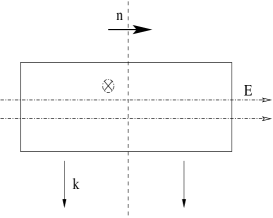
Figure 1: The experimental setup for detecting spin polarization and dichroism. The electric field, $E$, is normal to the Mirror plane. Both measured direction $k$ and the light are in the mirror plane.

All of the above four quantities are proportional to $\Delta M^{h}(\vec{k},\sigma(\vec{m}),\lambda)$ for each given band. In particular, we define the spin polarization when both $\vec{k}$ and $\vec{m}$ are in the mirror plane

$$P(\vec{k})=\sum_{a=r,l}I^{a}(\vec{k},\sigma(\vec{m}))-I^{a}(\vec{k},-\sigma(\vec{m}))$$ (23)

and the dichroism when $\vec{k}$ is in the mirror plane,

$$D(\vec{k})=\sum_{\sigma}(I^{r}(\vec{k},\sigma)-I^{l}(\vec{k},\sigma))$$ (24)

Both $P$ and $D$ are proportional to $\Delta M^{h}(\vec{k},\sigma(\vec{m}),\lambda)$, i.e.

$$P(\vec{k}),D(\vec{k})\propto\Delta M^{h}(\vec{k},\sigma(\vec{m}),\lambda)$$ (25)

Since both above quantities are proportional to external electric field, it is easy to verify whether the spin polarization and dichroism can be induced by the electric field experimentally. In a material without a mirror plane, it is still possible to detect the effect by observing the change of $P$ and $D$ according to the electric field although their values are not zero in general at zero field.

In conclusion, we have shown that electric field can induce spin polarization and dichroism effects in spin orbit coupling systems in ARPES. They share the same physical origins as the spin Hall effect. The values of the effects are exact opposite in the two bands which are split by spin orbit coupling. Since the spin polarization and dichroism effects are detected by completely different ARPES experiments, our predictions can be independently checked, which is crucial to resolve the present controversy regarding the existence of the spin Hall effect.

The author would like to thank Z. X. Shen, D. L. Feng and N. P. Armitage for valuable discussions. This work is supported by Purdue research funding.

References

- (1) S. Murakami, N. Nagaosa, and S.-C. Zhang, Science 301, 1348 (2003).
- (2) J. Sinova et al., Phys. Rev. Lett. 92, 126603 (2004).
- (3) J. Hu, B. A. Bernevig, and C. J. Wu, Int. J. Mod. Phys. B 17, 5991 (2003).
- (4) B. A. Bernevig, J. Hu, E. Mukamel, and S.-C. Zhang, Phys.Rev. B 70, 113301 (2004).
- (5) D. Culcer et al., Phys. Rev. Lett 93, 046602 (2004).
- (6) E. I. Rashba, Phys. Rev. B 68, 241315 (2003).
- (7) S. Murakami, N. Nagaosa, and S.-C. Zhang, Phys. Rev. B 69, 235206 (2004).
- (8) S. Murakami, N. Nagaosa, and S.-C. Zhang, Phys. Rev. Lett. 93, 156804 (2004).
- (9) S. Murakami, Phys. Rev. B 69, 241202 (2004).
- (10) E. I. Rashba, Phys. Rev. B 70, 201309 (2004).
- (11) B. A. Bernevig and S.-C. Zhang, cond-mat/0412550 (2004).
- (12) A. A. Burkov, A. S. Nunez, and A. H. MacDonald, Phys. Rev. B 70, 155308 (2004).
- (13) M.-C. Chang, cond-mat/0411697 (2004).
- (14) J. E. Hirsch, cond-mat/0406489 (2004).
- (15) J. Schliemann and D. Loss, Phys. Rev. B 68, 165311 (2003).
- (16) J. Schliemann and D. Loss, Phys. Rev. B 69, 165315 (2004).
- (17) N. A. Sinitsyn, E. M. Hankiewicz, W. Teizer, and J. Sinova, Phys. Rev. B 70, 081312 (2004).
- (18) S.-Q. Shen, Y.-J. Bao, M. Ma, X. Xie, and F. C. Zhang, cond-mat/0410169 (2004).
- (19) L. Sheng, D. N. Sheng, and C. S. Ting, cond-mat/0409038 (2004).
- (20) S. Y. Liu and X. L. Lei, cond-mat/0411629 (2004).
- (21) Y. K. Kato, R. C. Myers, A. C. Gossard, and D. Awschalom, Science (online) (2004).
- (22) J. Wunderlich, B. Kaestner, J. Sinova, and T. Jungwirth, cond-mat/0410295 (2004).
- (23) E. Mishchenko, A. Shytov, and B. Halperin, phys. Rev. Lett 93, 226602 (2004).
- (24) J. Inoue, G. Bauer, and L. Molenkamp, Phys. Rev. B 70, 41303 (2004).
- (25) A. Damascelli, Z. Hussain, and Z.-X. Shen, Rev. Mod. Phys 75, 473 (2003).
- (26) T. Mizokawa et al., Phys. Rev. Lett 87, 77202 (2001).
- (27) E. Rotenberg, J. W. Chung, and S. D. Kevan, Phys. Rev. Lett 82, 4066 (1999).