Effective charging energy for a regular granular metal array

Abstract

We study the Ambegaokar-Eckern-Schön (AES) model for a regular array of metallic grains coupled by tunnel junctions of conductance $g$ and calculate both paramagnetic and diamagnetic terms in the Kubo formula for the conductivity. We find analytically, and confirm by numerical path integral Monte Carlo methods, that for $0<g<4$ the conductivity obeys an Arrhenius law $\sigma(T)\sim\exp[-E^{*}(g)/T]$ with an effective charging energy $E^{*}(g)$ when the temperature is sufficiently low, due to a subtle cancellation between $T^{2}$ inelastic-cotunneling contributions in the paramagnetic and diamagnetic terms. We present numerical results for the effective charging energy and compare the results with recent theoretical analyses. We discuss the different ways in which the experimentally observed $\sigma(T)\sim\exp[-\sqrt{T_{0}/T}]$ law could be attributed to disorder.

The novel aspect of granular metals, which has attracted much experimentalSheng et al. (1973); Chui et al. (1981); Simon et al. (1987); Gerber et al. (1997); Beverly et al. (2002) and theoreticalEfetov and Tschersich (2002, 2003); Altland et al. (2004) interest, is the interplay between charging effects and incoherent intergrain hopping. One of the main questions concerns the manner and extent to which intergrain tunneling delocalizes the charge in the low-temperature limit. In the limit of $g\rightarrow 0,$ charging effects are dominant, implying an Arrhenius law for $\sigma(T)$. Furthermore, even in the case of large $g$ and low temperatures, heuristic arguments for a one-dimensional chain based on the partition function of the AES modelAltland et al. (2004) suggested an Arrhenius conductivity $\sigma(T)\sim\exp[-E^{*}(g)/T]$ at low temperatures with an effective charging energy $E^{*}(g)\sim E_{c}\exp[-\pi g/2].$ On the other hand, the conductance of a single quantum dot between two leads is dominated at low temperatures by inelastic cotunnelingAverin and Nazarov (1990), which gives a power-law temperature dependence.

We report several findings in this paper. First, for an ordered granular array we find that even as $g$ becomes large, the conductivity in the AES model remains Arrhenius-like although the Coulomb gap is exponentially small in $g$, and therefore, the localization length of the charge shows no increase with decrease in temperature. This is despite the fact that intergrain correlation functions indeed have a power-law temperature dependence due to inelastic cotunneling processes. We explicitly trace this apparent paradox to a subtle cancellation of the anomalous power-law dependences in the Kubo formula for conductivity. This result is expected to hold for any dimensionality of the ordered array, and has been verified numerically for a 1D array for $0<g<4$. Our results are consistent with experimentBeverly et al. (2002) and with recent theoretical workAltland et al. (2004); Arovas et al. (2003). Second, in view of the recent theoretical differences in the literature regarding the magnitude of $E^{*}(g)$, we also report the first numerical estimates for $E^{*}(g)$ for a regular array, extracted directly from the Kubo formula, which we expect will help resolve the theoretical issues. Finally, we also discuss the manner in which strong disorder in the grains’ background potential and in intergrain tunneling conductance affect our conclusions, especially in light of the experimentally observed soft-activation behavior $\sigma(T)\sim\exp[-\sqrt{T_{0}/T}]$ in disordered granular systems.

The Ambegaokar-Eckern-Schön (AES) modelAmbegaokar et al. (1982); Efetov and Tschersich (2002, 2003) is a valid description of a granular metal at temperatures higher than $\text{max}(g\delta,\delta)$ where $\delta$ is the mean level spacing at the Fermi energy in each grain. We begin with the AES model for a regular array of metallic grains,

$$S[\varphi] = S_{c}[\varphi]+S_{t}[\varphi]=\frac{1}{4E_{c}}\sum_{\text{{{x}}}}\int_{\tau}(\partial_{\tau}\varphi_{\tau\text{{{x}}}})^{2}+$$ (1)

$$+ \pi g\sum_{\text{{{xa}}}}\int_{\tau\tau^{\prime}}\alpha_{\tau-\tau^{\prime}}\sin^{2}\frac{\varphi_{\tau\text{{{x}}a}}-\varphi_{\tau^{\prime}\text{{{xa}}}}}{2},$$

where $\tau$ is imaginary time, x labels the grain positions, a is a unit lattice vector, $\varphi_{\tau\text{{{xa}}}}=\varphi_{\tau\text{{{x}}}}-\varphi_{\tau\text{{{x+a}}}},$ and the dissipation kernel $\alpha_{\tau}=T^{2}/\sin^{2}[\pi T(\tau+i\epsilon)].$ The Matsubara fields $\varphi_{\tau\text{{{x}}}}$ satisfy bosonic boundary conditions, $\varphi_{\beta\text{{{x}}}}=2\pi k_{\text{{{x}}}}+\varphi_{0\text{{{x}}}},$ where $k_{\text{{{x}}}}\in\mathbb{Z}$ is the winding number at site $\mathbf{x}.$ The model describes transport in a granular metal as a competition of charging ($S_{c}[\varphi]$) and dissipative intergrain tunneling ($S_{t}[\varphi]$).

For convenience we now define the site correlator ${\mathcal{C}}_{\tau_{1}\tau_{2}}={\mathcal{C}}_{\tau_{1}-\tau_{2}}=\langle\cos(\varphi_{\tau_{1}\text{{{x}}}}-\varphi_{\tau_{2}\text{{{x}}}})\rangle$ and the bond correlator $\Pi_{\tau_{1}\tau_{2}}=\Pi_{\tau_{1}-\tau_{2}}=\langle\cos(\varphi_{\tau_{1}\text{{{xa}}}}-\varphi_{\tau_{2}\text{{{xa}}}})\rangle.$

The electromagnetic response function ${\mathcal{K}}=d\langle j\rangle/dA$ is given by the Kubo formula. It consists of diamagnetic (${\mathcal{K}}^{d}$) and paramagnetic (${\mathcal{K}}^{p}$) contributions (${\mathcal{K}}={\mathcal{K}}^{d}+{\mathcal{K}}^{p}$). In units of $a^{2-d}(e^{2}/h),$

$${\mathcal{K}}_{\tau}^{d} = \pi g\left[{\mathcal{D}}_{\tau_{0},\tau_{0}+\tau}-\delta(\tau^{\prime})\int_{\tau^{\prime}}{\mathcal{D}}_{\tau_{0},\tau_{0}+\tau^{\prime}}\right],$$

where $${\mathcal{D_{\tau}}}=\alpha_{\tau}\Pi_{\tau},$$ (2)

$${\mathcal{K}}_{\tau}^{p} = \sum_{\text{{{x}}}}\left\langle\hat{j}_{\tau_{0},\mathbf{x}_{0},\mathbf{a}_{0}}\hat{j}_{\tau_{0}+\tau,\mathbf{x}_{0}+\mathbf{x},\mathbf{a}_{0}}\right\rangle,$$

where $$\hat{j}_{\tau_{1},\mathbf{x},\mathbf{a}}=\pi g\int_{\tau}\alpha_{\tau-\tau_{1}}\sin(\varphi_{\tau\mathbf{xa}}-\varphi_{\tau_{1}\mathbf{xa}}),$$ (3)

where $\Pi$ is the bond correlator of phases on adjacent grains at different times, and $\tau_{0},\mathbf{x}_{0},\mathbf{a}_{0}$ may be chosen arbitrarily. The real part of the conductivity is related to the imaginary part of the response function,

$$\text{Re }\sigma_{\omega} = \text{Im }\left[\frac{{\mathcal{K}}_{\omega}^{d}+{\mathcal{K}}_{\omega}^{p}}{\omega}\right].$$ (4)

The Kubo formula Eq.(4) only gives the part of the conductivity that is Ohmic and “extensive”, i.e., $\sigma=\lim_{L,A\rightarrow 0}(GL/A),$ where $G=\lim_{V\rightarrow 0}(I/V)$ is the zero bias conductance of the sample of length $L$ and cross section area $A.$ In a specimen of finite size, there are other contributions to the current (e.g., inelastic cotunneling) that are missed out by the Kubo formula.

Next we proceed to calculate the conductivity beginning with small values of intergrain conductance $g.$ In this case, the conductivity may be expanded in a perturbation series in $g.$ To the lowest order in $g$, only the diamagnetic part of the electromagnetic response matters, and it is straightforward to show using Eq.(2) and Eq.(4) that the d.c. conductivity is

$$\frac{\sigma^{d}}{\sigma_{0}}\approx 2e^{-\beta E_{c}}+2\beta E_{c}\,e^{-2\beta E_{c}}.$$ (5)

We now perform perturbation theory in $g$ for the site and bond correlators, taking $S_{c}[\varphi]$ as the bare action and $S_{t}[\varphi]$ as the perturbation. The first-order correction to the site correlator can be expressed in terms of bare correlators (the angle brackets represent expectations under the bare action):

$$\!\!\!\!\mathcal{C}_{\tau_{1}\tau_{2}\mathbf{x}_{1}}^{(1)} = \frac{\pi g}{2}\sum_{\mathbf{x}_{3}\mathbf{a}_{3}}\int\!\!\!\!\int_{\tau_{3}\tau_{4}}\alpha_{\tau_{3}-\tau_{4}}\times$$ (6)

$$\times \left[\left\langle e^{i(\varphi_{\tau_{1}\mathbf{x}_{1}}-\varphi_{\tau_{2}\mathbf{x}_{1}})}e^{i(\varphi_{\tau_{3}\mathbf{x}_{3}\mathbf{a}_{3}}-\varphi_{\tau_{4}\mathbf{x}_{3}\mathbf{a}_{3}})}\right\rangle-\right.$$

$$- \left.\left\langle e^{i(\varphi_{\tau_{1}\mathbf{x}_{1}}-\varphi_{\tau_{2}\mathbf{x}_{1}})}\right\rangle\left\langle e^{i(\varphi_{\tau_{3}\mathbf{x}_{3}\mathbf{a}_{3}}-\varphi_{\tau_{4}\mathbf{x}_{3}\mathbf{a}_{3}})}\right\rangle\right].$$

The first exponential in Eq.(6) involves phases on grain $\mathbf{x}_{1}$ while the second exponential involves phases on grains $\mathbf{x}_{3}$ and $\mathbf{x}_{4}=\mathbf{x}_{3}+\mathbf{a}_{3}.$ The averages in Eq.(6) can be factorized into averages over phases on separate grains.

(a) If $\mathbf{x}_{1},\,\mathbf{x}_{3}\,\,\text{and }\mathbf{x}_{4}$ are all distinct, the two expectations cancel each other exactly.

(b) If $\mathbf{x}_{1}=\mathbf{x}_{3}$ (or equivalently, if $\mathbf{x}_{1}=\mathbf{x}_{4}$), the integrand becomes $(\mathcal{C}_{\tau_{1}\tau_{2}\tau_{3}\tau_{4}}-\mathcal{C}_{\tau_{1}\tau_{2}}\mathcal{C}_{\tau_{3}\tau_{4}})\mathcal{C}_{\tau_{3}\tau_{4}},$ in terms of the bare single-grain correlators $\mathcal{C}$ and $\mathcal{C}_{\tau_{1}\tau_{2}\tau_{3}\tau_{4}}=\left\langle e^{i(\varphi_{\tau_{1}}-\varphi_{\tau_{2}}+\varphi_{\tau_{3}}-\varphi_{\tau_{4}})}\right\rangle$.

$\mathcal{C}_{\tau_{1}\tau_{2}\tau_{3}\tau_{4}}$ takes its largest value, 1, when $\tau_{1}\approx\tau_{2}$ and $\tau_{3}\approx\tau_{4}$, or when $\tau_{1}\approx\tau_{4}$ and $\tau_{3}\approx\tau_{2}$; it decays exponentially with $|\tau_{1}-\tau_{2}|$, etc. This behavior is approximately described by Wick’s theorem, $\mathcal{C}_{\tau_{1}\tau_{2}\tau_{3}\tau_{4}}\approx\mathcal{C}_{\tau_{1}\tau_{2}}\mathcal{C}_{\tau_{3}\tau_{4}}+\mathcal{C}_{\tau_{1}\tau_{4}}\mathcal{C}_{\tau_{3}\tau_{2}};$ however, when all the time indices are equal, $\mathcal{C}_{\tau_{1}\tau_{2}\tau_{3}\tau_{4}}=1$ (not $2$). We handle this by defining $\alpha_{\tau_{3}-\tau_{4}}^{\text{reg}}$ as $\alpha_{\tau_{3}-\tau_{4}}$ times a regularizing factor that vanishes at $\tau_{3}=\tau_{4}$:

$$\mathcal{C}_{\tau_{1}\tau_{2}\mathbf{x}_{1}}^{(1)} = \frac{\pi gz}{2}\int\!\!\!\!\int_{\tau_{3}\tau_{4}}\alpha_{\tau_{3}-\tau_{4}}^{\text{reg}}\mathcal{C}_{\tau_{1}\tau_{4}}\mathcal{C}_{\tau_{3}\tau_{2}}\mathcal{C}_{\tau_{3}\tau_{4}}$$ (7)

$$\approx \frac{\pi gz}{2}\left(\frac{2}{E_{c}}\right)^{2}\alpha_{\tau_{1}-\tau_{2}}^{\text{reg}}\mathcal{C}_{\tau_{1}\tau_{2}}.$$

where $z$ is the coordination number of the grain. This is exponentially small ($\sim\exp[-E_{c}|\tau_{1}-\tau_{2}|]$). Thus to first order in $g,$ the exponential decay of the site correlator is not changed, in contrast with the case of the bond correlator that we now discuss.

The first correction to the bond correlator is

$$\!\!\!\!\!\!\!\!\!\mathcal{C}_{\tau_{1}\tau_{2}\mathbf{x}_{1}\mathbf{a}}^{(1)} = \frac{\pi g}{2}\sum_{\mathbf{x}_{3}\mathbf{a}_{3}}\int\!\!\!\!\int_{\tau_{3}\tau_{4}}\alpha_{\tau_{3}-\tau_{4}}\times$$ (8)

$$\!\!\!\!\!\!\!\!\!\!\times \!\!\!\!\!\!\!\left[\left\langle e^{i(\varphi_{\tau_{1}\mathbf{x}_{1}\mathbf{a}_{1}}-\varphi_{\tau_{2}\mathbf{x}_{1}\mathbf{a}_{1}})}e^{i(\varphi_{\tau_{3}\mathbf{x}_{3}\mathbf{a}_{3}}-\varphi_{\tau_{4}\mathbf{x}_{3}\mathbf{a}_{3}})}\right\rangle-\!\!\!\!\right.$$

$$\!\!\!\!\!\!\!\!\!\!- \!\!\!\!\!\!\!\!\!\left.\left\langle e^{i(\varphi_{\tau_{1}\mathbf{x}_{1}\mathbf{a}_{1}}-\varphi_{\tau_{2}\mathbf{x}_{1}\mathbf{a}_{1}})}\right\rangle\!\!\left\langle e^{i(\varphi_{\tau_{3}\mathbf{x}_{3}\mathbf{a}_{3}}-\varphi_{\tau_{4}\mathbf{x}_{3}\mathbf{a}_{3}})}\right\rangle\right].$$

The first exponential in Eq.(8) involves phases on grains $\mathbf{x}_{1}$ and $\mathbf{x}_{2}=\mathbf{x}_{1}+\mathbf{a}_{1},$ while the second exponential involves phases on grains $\mathbf{x}_{3}$ and $\mathbf{x}_{4}=\mathbf{x}_{3}+\mathbf{a}_{3}.$ This is illustrated in Fig.1.

(a) If the two bonds do not share a common site, the expectation of the product of the cosines of the phases on these bonds factorizes. Hence the two terms cancel and there is no expectation.

(b) If the two bonds have one site in common, such that $\mathbf{x}_{1}=\mathbf{x}_{3}$ for example, then the integrand becomes $({\cal C}_{\tau_{1}\tau_{2}\tau_{3}\tau_{4}}-{\cal C}_{\tau_{1}\tau_{2}}{\cal C}_{\tau_{3}\tau_{4}}){\cal C}_{\tau_{3}\tau_{4}}.$

(c) If the two bonds have both sides in common, i.e., $\mathbf{x}_{1}=\mathbf{x}_{3}$ and $\mathbf{x}_{2}=\mathbf{x}_{4}$ (and $\mathbf{a}_{1}=\mathbf{a}_{3}$), then the integrand is $({\cal C}_{\tau_{1}\tau_{2}\tau_{3}\tau_{4}})^{2}-({\cal C}_{\tau_{1}\tau_{2}})^{2}({\cal C}_{\tau_{3}\tau_{4}})^{2}.$

Figure 1: Contributions to the bond correlator $\Pi_{\tau\mathbf{a}}.$ (a) No sites in common, (b) one common site, and (c) two common sites.

The second term in case (c) is always small ($\sim\exp[-2E_{c}|\tau_{1}-\tau_{2}|]$), but the first contains peaks when its four arguments can be partitioned into even-odd pairs of $\tau$’s that are close to each other. Hence when performing the integral over $\tau_{3}$ and $\tau_{4},$ one finds an important contribution from the region where $|\tau_{1}-\tau_{4}|$ and $|\tau_{2}-\tau_{3}|$ are small:

$$\mathcal{C}_{\tau_{1}\tau_{2}\mathbf{x}_{1}\mathbf{a}_{1}}^{(1c)}=\frac{\pi g}{2}\int\!\!\!\!\int_{\tau_{3}\tau_{4}}\!\!\!\!\alpha_{\tau_{3}-\tau_{4}}(\mathcal{C}_{\tau_{1}\tau_{2}\tau_{3}\tau_{4}})^{2}\approx\frac{2\pi g}{E_{c}^{2}}\alpha_{\tau_{1}-\tau_{2}}.$$ (9)

In accordance with Griffiths’ theorem Griffiths (1967); Ginibre (1970), the long-ranged interaction produces a qualitative change in the behavior of the correlation function.

Putting $\Pi_{\tau\mathbf{a}}$ into the expression for the diamagnetic response $\mathcal{K}^{d}$ gives the second order correction to $\mathcal{K}^{d}:$

$$\mathcal{K}_{\tau}^{d(2)} \approx \frac{2\pi^{2}g^{2}}{E_{c}^{2}}\left[\alpha_{\tau}^{2}-\delta(\tau)\int_{\tau^{\prime}}\alpha_{\tau^{\prime}}^{2}\right].$$ (10)

This contributes to the conductivity a term proportional to $g^{2}T^{2}$ at low temperatures — a much weaker insulating behavior than both Arrhenius ($\exp[-E_{c}/T]$) and soft activation ($\exp[-\sqrt{T_{0}/T}]$) laws commonly encountered in experiment. This is reminiscent of inelastic cotunneling processes, which are known to give a conductance proportional to $T^{2}$ for a single quantum dotAverin and Nazarov (1990); however, the conductivity of a granular metal is related to the conductance of a macroscopic specimen, and in order to contribute to this conductance, $L$ electrons would have to cotunnel simultaneously along each segment of the path linking one electron to the other, which would give a negligible conductance proportional to $T^{2L}.$ In order to obtain the correct behavior one must also consider the paramagnetic contribution.

The first term of $\mathcal{K}^{p}$ is also proportional to $g^{2}$ and can be calculated from the bare action. From Eq.(3),

$$\mathcal{K}_{\tau_{1}\tau_{3}\mathbf{x}_{1}\mathbf{x}_{3}\mathbf{a}_{1}\mathbf{a}_{3}}^{p}=\pi^{2}g^{2}\int\!\!\!\!\int_{\tau_{2}\tau_{4}}\alpha_{\tau_{1}-\tau_{2}}\alpha_{\tau_{3}-\tau_{4}}\times\qquad$$

$$\times\langle\sin(\varphi_{\tau_{1}\mathbf{x}_{1}\mathbf{a}_{1}}-\varphi_{\tau_{2}\mathbf{x}_{1}\mathbf{a}_{1}})\sin(\varphi_{\tau_{3}\mathbf{x}_{3}\mathbf{a}_{3}}-\varphi_{\tau_{4}\mathbf{x}_{3}\mathbf{a}_{3}})\rangle.$$ (11)

The first sine involves phases on grains $\mathbf{x}_{1}$ and $\mathbf{x}_{2}=\mathbf{x}_{1}+\mathbf{a}_{1},$ while the second sine involves the phases on grains $\mathbf{x}_{3}$ and $\mathbf{x}_{4}=\mathbf{x}_{3}+\mathbf{a}_{3}.$ Marking these bonds on the lattice gives the same picture as Fig.1.

(a) If these bonds do not share a common site, the average is zero by symmetry.

(b) If the bonds share one common site, the average is still zero.

(c) The only finite contribution arises when these bonds have both sites in common. In this case, the term in the angle brackets in Eq.(11) gives

$$\mathcal{K}_{\tau_{1}\tau_{3}\mathbf{x}_{1}\mathbf{x}_{3}\mathbf{a}_{1}\mathbf{a}_{3}}^{p} = -\frac{\pi^{2}g^{2}}{2}\int\!\!\!\!\int_{\tau_{2}\tau_{4}}\alpha_{\tau_{1}-\tau_{2}}\alpha_{\tau_{3}-\tau_{4}}\times$$ (12)

$$\times[(\mathcal{C}_{\tau_{1}\tau_{2}\tau_{3}\tau_{4}})^{2}-(\mathcal{C}_{\tau_{1}\tau_{2}\tau_{4}\tau_{3}})^{2}].$$

When $|\tau_{1}-\tau_{2}|$ and $|\tau_{3}-\tau_{4}|$ are small, the two correlators in Eq.(12) cancel out. When $|\tau_{1}-\tau_{4}|$ and $|\tau_{2}-\tau_{3}|$ are small, integration over $\tau_{2}$ and $\tau_{4}$ gives $-(2\pi^{2}g^{2}/E_{c}^{2})\alpha_{\tau_{1}-\tau_{3}}.$ When $|\tau_{1}-\tau_{3}|$ and $|\tau_{2}-\tau_{4}|$ are small, performing the integration gives $(2\pi^{2}g^{2}/E_{c}^{2})\delta(\tau_{1}-\tau_{3})\int_{\tau^{\prime}}\alpha_{\tau^{\prime}}^{2}.$ Gathering these results, the correction to $\mathcal{K}_{\tau}^{p}$ at large $\tau$ is

$$\mathcal{K}_{\tau}^{p(2)} \approx -\frac{2\pi^{2}g^{2}}{E_{c}^{2}}\left[\alpha_{\tau}^{2}-\delta(\tau)\int_{\tau^{\prime}}\alpha_{\tau^{\prime}}^{2}\right].$$ (13)

This is equal and opposite to the correction to $\mathcal{K}^{d},$ Eq.(10). Hence the anomalous $T^{2}$ terms in the conductivity cancel out when all contributions are taken into account.

For $1\lesssim g<4$, where perturbation theory in $g$ is not justified, we have computed $\mathcal{K}_{\tau}^{d}$ and $\mathcal{K}_{\tau}^{p}$ using a path integral Monte Carlo approach (see Fig.2). At sufficiently long times, $E_{c}^{*}(g)\tau\gg 1,$ both these functions have anomalous $1/\tau^{2}$ dependences, but these cancel, leaving behind an exponentially small $\mathcal{K}_{\tau}.$

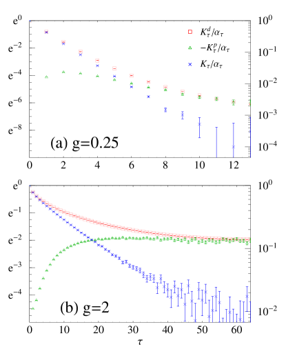
Figure 2: (Color online) Monte Carlo estimates of electromagnetic response functions (scaled by $\alpha_{\tau}$) for a ring of 16 grains with $E_{c}=\frac{1}{2}$ and $\beta=128$. The anomalous power-law contributions in ${\cal K}_{\tau}^{d}/\alpha_{\tau}$ and ${\cal K}_{\tau}^{p}/\alpha_{\tau}$ exactly cancel out in ${\cal K}_{\tau}/\alpha_{\tau}$, leaving behind a small difference that obeys the Arrhenius law, $\exp[-E_{*}(g)\tau].$

The numerical data show that $\mathcal{C}_{\tau}$ and $\mathcal{K}_{\tau}/\alpha_{\tau}$ decay exponentially, but the effective charging energies ($E^{**}$ and $E^{*}$ respectively) are reduced from $E_{c}$. Fig. 3 shows our estimates of $E^{*}$ and $E^{**}$. The site correlator has a gap that approximately obeys $E^{**}(g)\approx E_{c}e^{-\pi g/4}$. In our earlier papersTripathi et al. (2004); Loh et al. (2005), we have proposed that for a single junction, the characteristic energy is $T_{*}\sim E_{c}e^{-\pi g/2}$. This has a simple physical interpretation. Delocalization of the charge over $N$ grains reduces the charging energy to $E_{c}/N$, however the probability of correlating the phases on $N$ neighboring grains decreases exponentially as $p_{N}\sim p_{1}^{N}\sim e^{-NT_{*}/T}$. Optimizing with respect to $N$ gives the probability of single-charge excitation for a granular chain, $p\sim e^{-2\sqrt{T_{*}E_{c}}}$, i.e., $E^{**}(g)=\sqrt{T_{*}E_{c}}\sim E_{c}e^{-\pi g/4}$. This result of ours for $E^{**}(g)$ would agree with the analysis in Ref.Altland et al. (2004) if the single-junction characteristic energy is taken to be $T_{*}\sim E_{c}e^{-\pi g/2}$ instead of $E_{c}e^{-\pi g}$ used in Ref.Altland et al. (2004). The characteristic energy for a 1D granular chain thus differs from that inferred from the analysis in Ref.Efetov and Tschersich (2002). The effective Arrhenius gap for the conductivity, $E^{*}(g)$ fits well to $E^{*}(g)\approx E_{c}e^{-g}$ and differs from existing analytical predictions. We cannot rule out numerical subtleties causing the difference between $E^{*}(g)$ and $E^{**}(g)$.

Renormalization group calculations (Refs.Efetov and Tschersich (2003); Falci et al. (1995)) for a single electron box show that the conductance $g>1$ always renormalizes to lower values as temperature is reduced. If the same statement holds for the AES model for the granular array, and there is no a priori reason why it should, the implication is that the regular AES model has an Arrhenius conductivity at low temperatures regardless of how large $g$ is.

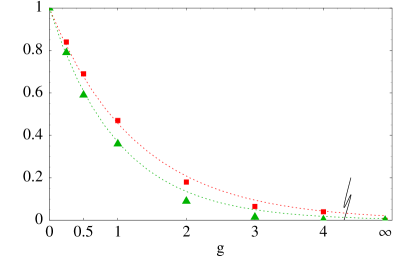
Figure 3: (Color online) Effective charging energies $E^{**}(g)$ (squares) and $E^{*}(g)$ (triangles), estimated from decay constants of $\mathcal{C}_{\tau}$ and $\mathcal{K}_{\tau}/\alpha_{\tau}$ respectively. Dotted lines are $e^{-\pi g/4}$ and $e^{-g}$. At large $g$ ($\geq 3$), estimates suffer from error due to (i) discretization, (ii) insufficiently large $\beta$.

The physical picture emerging from our calculation is that for an ordered array, sequential cotunneling processes which take charge around a loop make anomalous contributions to certain intergrain correlation functions but not to the conductivity. The conclusion is that anomalous behavior in conductivity, such as soft activation or $T^{2}$, should not be automatically inferred from anomalous behavior in certain correlation functions or in the partition function.

We conclude with a discussion of disorder effects. Experiments on disordered 2D and 3D granular metalsSheng et al. (1973); Chui et al. (1981); Simon et al. (1987); Gerber et al. (1997) often reveal a ‘soft-activation’ law $\sigma(T)\sim\exp[-\sqrt{T_{0}/T}]$. More recently, the conductivity of carefully prepared nanoparticle arrays with controllable disorder Beverly et al. (2002) has been found to follow an Arrhenius law $\sigma(T)\sim\exp[-E^{*}/T]$ for ordered arrays, crossing over to soft-activation behavior with increased disorder in the position and size of the grains. Another relevant source of disorder is impurities in the insulating substrate which create random gate voltages $V_{g\mathbf{i}}$ at the grains. The presence of such disorder reduces the typical charging energy of the grains; in particular, the charging energy vanishes when the grain background charge $Q_{0\mathbf{i}}=C_{\mathbf{i}}V_{g\mathbf{i}}=\frac{1}{2}$. This in turn makes energy levels available in the entire range $[-E_{c}/2,E_{c}/2]$. In combination with inelastic cotunneling, variable-range hopping can lead to a Mott or Efros-ShklovskiiEfros and Shklovskii (1975) law for conductivity. This differs from the original Efros-Shklovskii mechanism in that variable-range hopping due to wavefunction overlap is replaced by variable-length sequences of inelastic cotunneling eventsFeigel’man and Ioselevich (2005). In our previous workTripathi et al. (2004), we recognized the importance of cotunneling over many grains in an eventual explanation for the soft-activation behavior. However, as we have shown in this paper, cotunneling by itself is insufficient, and only Arrhenius conductivity is possible for arrays without disorder.

It is also possible to create a range of energy levels in the interval $[-E_{c}/2,E_{c}/2]$ through strong disorder in intergrain tunneling. In particular, if in some part of the system, the intergrain tunneling is large, then, as we have just shown, the charging energy is exponentially small, $E^{**}(g)\sim E_{c}e^{-\pi g/4}$ for a chain and even smaller for higher dimensional arrays. Since actual experiments are performed at not too low temperatures $T>\delta\sim O(1K)$, we only need to make puddles available up to charging energies as low as $E^{**}(g)=\delta$. This is plausible if tunneling disorder is strong so that all conductances in the puddle are larger than $g>(4/z\pi)\ln(E_{c}/\delta)$. Once again, variable-range hopping arguments in combination with inelastic cotunneling will lead to a soft activation law. This could be an independent possibility in the position-disordered arrays in Ref. Beverly et al., 2002. In the presence of background charge disorder, even positionally regular arrays will show soft-activation behavior. An explicit calculation of the conductivity for the disordered AES model will be taken up in a forthcoming work.

YLL thanks Trinity College, Cambridge and the Cavendish Laboratory for support. VT thanks Trinity College for a JRF.

References

• Sheng et al. (1973) P. Sheng, B. Abeles, and Y. Arie, Phys. Rev. Lett. 31, 44 (1973).
• Chui et al. (1981) T. Chui, G. Deutscher, P. Lindenfeld, and W. L. McLean, Phys. Rev. B 23, R6172 (1981).
• Simon et al. (1987) R. W. Simon, B. J. Dalrymple, D. Van Vechten, W. W. Fuller, and S. A. Wolf, Phys. Rev. B 36, 1962 (1987).
• Gerber et al. (1997) A. Gerber, A. Milner, G. Deutscher, M. Karpovsky, and A. Gladkikh, Phys. Rev. Lett. 78, 4277 (1997).
• Beverly et al. (2002) K. C. Beverly, J. F. Sampaio, and J. R. Heath, J. Phys. Chem. B 106, 2131 (2002).
• Efetov and Tschersich (2002) K. B. Efetov and A. Tschersich, Europhysics Lett. 59, 114 (2002).
• Efetov and Tschersich (2003) K. B. Efetov and A. Tschersich, Phys. Rev. B 67, 174205 (2003).
• Altland et al. (2004) A. Altland, L. I. Glazman, and A. Kamenev, Phys. Rev. Lett. 92, 026801 (2004).
• Averin and Nazarov (1990) D. V. Averin and Y. V. Nazarov, Phys. Rev. Lett. 65, 2446 (1990).
• Arovas et al. (2003) D. P. Arovas, F. Guinea, C. P. Herrero, and P. San Jose, Phys. Rev. B 68, 085306 (2003).
• Ambegaokar et al. (1982) V. Ambegaokar, U. Eckern, and G. Schön, Phys. Rev. Lett. 48, 1745 (1982).
• Griffiths (1967) R. B. Griffiths, J. Math. Phys. 8, 478 (1967).
• Ginibre (1970) J. Ginibre, Commun. Math. Phys. 16, 310 (1970).
• Tripathi et al. (2004) V. Tripathi, M. Turlakov, and Y.L.Loh, J. Phys. Cond. Mat. 16, 4867 (2004).
• Loh et al. (2005) Y. L. Loh, V. Tripathi, and M. Turlakov, Phys. Rev. B 71, 024429 (2005).
• Falci et al. (1995) G. Falci, G. Schön, and G. T. Zimanyi, Phys. Rev. Lett. 74, 3257 (1995).
• Efros and Shklovskii (1975) A. L. Efros and B. I. Shklovskii, J. Phys. C 8, L49 (1975).
• Feigel’man and Ioselevich (2005) M. V. Feigel’man and A. S. Ioselevich, cond-mat/0502481 (2005).