Surface-enhanced Raman scattering and fluorescence near metal nanoparticles

Abstract

We present a general model study of surface-enhanced resonant Raman scattering and fluorescence, focusing on the interplay between electromagnetic (EM) effects and the molecular dynamics as treated by a density matrix calculation. The model molecule has two electronic levels, is affected by radiative and non-radiative damping mechanisms, and a Franck-Condon mechanism yields electron-vibration coupling. The coupling between the molecule and the electromagnetic field is enhanced by placing it between two Ag nanoparticles. The results show that the Raman scattering cross section can, for realistic parameter values, increase by some 10 orders of magnitude (to $\sim 10^{-14}$ cm²) compared with the free-space case. Also the fluorescence cross section grows with increasing EM enhancement, however, at a slower rate, and this increase eventually stalls when non-radiative decay processes become important. Finally, we find that anti-Stokes Raman scattering is possible with strong incident laser intensities, $\sim 1$ mW/$\mu$m.

I Introduction

Surface-enhanced Raman scattering (SERS) was discovered three decades ago. SERS attracted a lot of attention through the mid-1980’s.Review1 ; Review2 ; SPIE During this period the basic mechanisms behind the effect were studied, explained, and debated. The advent of single-molecule (SM) SERSNie:97 ; Kneipp:97 ; Xu:99 ; Brus:99 started a second period of intense research. Now probably the prospect of utilizing SERS and related spectroscopic techniques as an extremely sensitive analytic tool, possibly combined with scanning probe techniques,TERS in a variety of life-science applicationsLakowicz:01 provides the main motivation for research in the field. But SM SERS experiments performed with intense lasers has also raised new questions about the fundamental mechanisms involved.Kneipp:96 ; Kneipp:98 ; Haslett:00 ; Brolo:04

It is generally agreed that electromagnetic (EM) enhancement effects are the most important reason for the dramatic increase of the Raman scattering cross-section $\sigma_{R}$ seen in SERS experiments. Mosk:78 ; Gersten:80 ; Takemori:87 ; GV:96 ; Xu:00 ; Corni:02 ; Stockman:03 In addition to this, $\sigma_{R}$ may also be enhanced due to charge transfer effects.Persson:81 ; Pettinger:86 ; Otto:89 ; Brus:99 ; Otto:02 The EM enhancement effects received a lot of attention from the theory side in the early days of SERS and has continued to do so until now. The electromagnetic enhancement has in the general case not one single reason, but involves several, more or less closely related aspects such as plasmon resonances, lightning rod effects, and the formation of “hot-spots” in fractal clusters.

However, single-molecule Raman scattering is not possible without a molecule that scatters the laser light inelastically. In this paper we focus on the interplay between the EM enhancement and molecular dynamics, a topic that has received relatively limited attention in the literature so far. A brief account of this work was published in Ref. Xu:04, . We treat the molecule as an electronic two-level system. Thus, we make no attempt of calculating ab initio molecular properties, and charge transfer processes are also outside the scope of this work. The focus is instead on calculating how the molecule’s different states are populated and how its coherent dipole moment develops given a certain energy-level structure, electron-vibration coupling, electromagnetic enhancement and laser intensity. By treating the molecule dynamics within a density-matrix calculation, we can evaluate a combined fluorescence and Raman spectrum where also effects of electromagnetic enhancement are directly included. Density-matrix methods were employed by ShenYRShen:74 to distinguish between Raman scattering and hot luminescence, but to the best of our knowledge they have not been used in the context of SERS.

The results show how, for a molecule placed between two metallic nanoparticles, both the fluorescence and in particular the Raman cross sections are much larger than for a molecule in free space. This can be discussed in terms of two EM enhancement factors, $M$ and $|M_{d}|$. Given an electric-field enhancement $M(\omega)$ at the position of the molecule, the Raman cross section increases by a factor $\sim|M|^{4}$ compared with in free space, whereas the fluorescence cross section increases by the factor $\sim|M|^{4}/|M_{d}|^{2}$. $|M_{d}|^{2}$ is a measure of how much the decay rate of an excited state of the molecule is amplified near one or several metal particles. For moderate to large molecule-particle distances $M$ and $|M_{d}|$ are almost equal, but when the molecule gets very close to a particle (a few nm or less) $|M_{d}|$ can be much larger than $M$. Thus, surface enhancement of fluorescence is much less marked than that of Raman scattering, and for small enough molecule-particle separations the fluorescence cross section saturates. When studying a molecule next to a single metal particle, $M$ does not reach at all as high values as in the two-particle case, but $|M_{d}|$ still does. Consequently, the SERS effect is largely absent in this case, and fluorescence is strongly quenched when the molecule is placed close to the particle. Distancing the molecule from the particle, $|M_{d}|$ drops and the fluorescence goes through a maximum and then eventually falls back to the free-molecule value.

We have also studied how the Raman spectrum develops when the intensity of the driving laser field is increased to relatively large values of order $1\mathrm{\,mW/(\mu m^{2})}$. In this case we find that anti-Stokes Raman scattering becomes possible even if the molecule vibrations are not thermally excited. Such effects have been observed in a number of SERS experiments, but the issue has been quite controversial.Kneipp:96 ; Kneipp:98 ; Haslett:00 We find that anti-Stokes Raman scattering in our model occurs because a vibrationally excited level in the electronic ground state is populated by (possibly repeated) excitation from the laser and subsequent deexcitation. We also find that when the laser intensity is increased to values where Rabi oscillations become important, the anti-Stokes Raman cross section decreases, and the corresponding peak in the spectrum broadens.

The rest of the paper is organized as follows. In Sec. II we describe the model for the molecule that we use. As already stated, the electromagnetic enhancement plays an important role in SERS, and Sec. III describes how the EM enhancement of the incident laser field, the emitted light, and the deexcitation of the molecule is calculated. Moreover, we also present numerical results for some representative cases. Then in Sec. IV we go back to the model molecule and investigate how the parameter values entering the model affect the absorption and Raman scattering cross sections for the molecule in free space. In Sec. V we use density-matrix theory to derive a general expression from which the combined fluorescence and Raman scattering spectrum can be calculated for a molecule placed near metal nanoparticles, and driven by, in principle, an arbitrarily strong laser field. The so calculated spectra are presented in Sec. VI, and Sec. VII concludes the paper with a brief comparison with experiments. Finally, Appendix A gives some background information about the electromagnetic calculations, and Appendix B presents a derivation of the non-radiative damping of the molecule due to electron-hole pair creation in the metal particles.

II Model

A schematic illustration of our model, both in terms of molecule-nanoparticle geometry and the main features of the molecule model is given in Fig. 1. In this figure we also indicate the main steps involved in different Raman and fluorescence processes.

Figure 1: Schematic illustration of the model we use. (a) Electromagnetic enhancement is achieved by (usually) placing the model molecule between two metallic nanoparticles. (b) The molecule has two electronic states (sometimes called bands in the following) each with a number of vibrational sublevels. The equilibrium position for the vibrational coordinate is displaced by $x_{0}$ upon electronic excitation; this mechanism provides electron-vibration coupling. The arrows indicate typical pathways for the molecule state in fluorescence and Raman processes.

We model the electronic degrees of freedom of the molecule as a two-level system with states $|g\rangle$ and $|e\rangle$. The frequency $\Omega_{ge}$, defined from the energy-level separation $E_{e}-E_{g}$ as

$$\hbar\Omega_{ge}=E_{e}-E_{g},$$ (1)

and the dipole matrix element, expressed as the product of the elementary charge $e_{e}$ and a dipole length $\ell_{\mathrm{dip}}$, $p_{0}=e_{e}\ell_{\mathrm{dip}}$, (to be further discussed below) are the only parameters we need in this context to characterize the essential electronic properties of the molecule.

To deal with Raman scattering we must of course introduce vibrational degrees of freedom and an electron-vibration coupling. We consider only one symmetric, vibrational mode, and let $Q$ denote the corresponding coordinate. The vibrational mode is characterized by its angular frequency $\Omega_{\mathrm{vib}}$ and reduced mass $\mu$. The purely vibrational Hamiltonian can thus be written

$$H_{\mathrm{vib}}=\hbar\Omega_{\mathrm{vib}}(b^{{\dagger}}b+\frac{1}{2}),$$ (2)

where $b$ and $b^{{\dagger}}$ are annihilation and creation operators for a vibrational quantum. We assume that the vibrational frequency is independent of the electron state, but the equilibrium position is displaced a distance $x_{0}$ in the excited state. Moreover, the transition dipole moment introduced above is actually a function of $Q$: in the Born-Oppenheimer approximation we get the Taylor expansion

$$p\equiv p(Q)=\langle e(Q)|e_{e}z|g(Q)\rangle=p_{0}+\left(\frac{dp}{dQ}\right)Q+\ldots,$$

around $Q=0$. (Thus, we focus on the $z$ components of the electric fields and dipole moments, since they are the ones enhanced in the nanoparticle geometry we study.) Then the dipole matrix element between two electron-vibration product states yields

$$\langle x_{0};m|\langle e|e_{e}z|g\rangle 0;n\rangle$$

$$=p_{0}\,\langle x_{0};m|0;n\rangle+\left(\frac{dp}{dQ}\right)\,\langle x_{0};m|Q|0;n\rangle+\ldots,$$ (3)

where $|x_{0};n\rangle$ denotes vibrational state $n$ in an oscillator potential with the equilibrium position displaced to $Q=x_{0}$, etc. We adopt the Condon approximation, thus retaining only the first (Albrecht $A$) termLombardi:86 in Eq. (3). It gives the dominating contribution in situations where the incident light is close to resonance with the electronic transition. We thus get

$$\langle x_{0};m|\langle e|e_{e}z|g\rangle 0;n\rangle=p_{0}f(n,m),$$ (4)

where the Franck-Condon factor

$$f(n,m)=\,\langle 0;n|x_{0};m\rangle=\,\langle x_{0};m|0;n\rangle$$

$$=\sqrt{n!m!}\,\,e^{-\alpha^{2}/2}\sum_{k=0}^{min(n,m)}\frac{(-1)^{(m+k)}\alpha^{n+m-2k}}{k!(n-k)!(m-k)!},$$ (5)

and the ratio $\alpha$ between $x_{0}$ and the average zero-point vibration, $(\langle(2Q)^{2}\rangle)^{1/2}=(2\hbar/(\mu\Omega_{\mathrm{vib}}))^{1/2}$,

$$\alpha=x_{0}\,\sqrt{\frac{\mu\Omega_{\mathrm{vib}}}{2\hbar}},$$ (6)

serves as a measure of the electron-vibration coupling in the model.

The molecule is furthermore interacting with the electromagnetic field, both with the incident laser field and the electromagnetic vacuum fluctuations that cause spontaneous emission. The electric field originating from the laser can be written

$$\vec{E}_{L}=\hat{z}E_{0}\cos{\Omega_{L}t}=\hat{z}({E_{0}}/{2})\,[e^{i\Omega_{L}t}+e^{-i\Omega_{L}t}],$$ (7)

so that the nominal incident intensity is $I_{\mathrm{in}}=c\varepsilon_{0}E_{0}^{2}/2.$ We model the laser-molecule interaction within the dipole approximation by a $-e_{e}\,\vec{r}\cdot\vec{E}$ term, $H^{\prime}=-e_{e}E_{0}z[e^{i\Omega_{L}t}+e^{-i\Omega_{L}t}]/2$ in the Hamiltonian. When evaluating matrix elements due to $H^{\prime}$ we adopt the rotating wave approximation (RWA). Only the part of the field varying with time as $e^{-i\Omega_{L}t}$ is kept in the matrix elements when the molecule is excited, and vice versa when it is deexcited. This yields

$$\langle x_{0};m|\langle e|H^{\prime}|g\rangle|0;n\rangle=-(p_{0}E_{0}/2)e^{-i\Omega_{L}t}\,f(n,m),$$ (8)

and

$$\langle 0;n|\langle g|H^{\prime}|e\rangle|x_{0};m\rangle=-(p_{0}E_{0}/2)e^{i\Omega_{L}t}\,f(n,m).$$ (9)

(In the following, when the local field at the molecule is modified by the nearby metallic particles, these matrix elements must be corrected by an enhancement factor.)

The interaction between the molecule and the vacuum fluctuations of the electromagnetic field can be described by a Hamiltonian $H_{\mathrm{fluct}}=-e_{e}zE_{\mathrm{vac}}\cdot\hat{z},$ where the corresponding electric field must be given on second-quantized form. In free space we have

$$\vec{E}_{\mathrm{vac}}(\vec{r},t)=\sum_{{\bf k},\alpha}\sqrt{\frac{\hbar}{2\epsilon\omega_{k}}}\frac{i\omega_{k}}{L^{3/2}}{\bf\varepsilon}_{{\bf k},\alpha}e^{i{\bf k}\cdot{\bf r}}[a_{{\bf k},\alpha}(t)-a_{{\bf k},\alpha}^{{\dagger}}(t)],$$ (10)

where the electromagnetic field has been normalized in a box with side $L$, and $a_{{\bf k},\alpha}$ and $a_{{\bf k},\alpha}^{{\dagger}}$ are annihilation and creation operators for photons. For a molecule in free space the interaction with the vacuum fluctuations gives a transition rate

$$\gamma_{\mathrm{rad},0}(n,m)=\frac{\omega^{3}}{3\pi\hbar\varepsilon_{0}c^{3}}|p_{0}|^{2}|f(n,m)|^{2},$$ (11)

where $\omega$ is the angular frequency corresponding to the transition energy, i.e.

$$\omega=\Omega_{ge}+(m-n)\omega_{\mathrm{vib}}.$$ (12)

With a dipole moment corresponding to $\ell_{\mathrm{dip}}=1$ Å, a transition energy of 2.5 eV, and $|f|^{2}=1$, we get numerically $\gamma_{\mathrm{rad},0}\approx 5.9\times 10^{7}\mathrm{\,s^{-1}}$.

This transition rate is enhanced when the molecule is placed near metallic nanoparticles; the radiative losses increase and in addition energy can be dissipated in the particles, thus

$$\gamma_{\mathrm{rad},0}(n,m)\rightarrow|M_{d}(\omega)|^{2}\gamma_{\mathrm{rad},0}(n,m).$$

We will discuss the dissipation enhancement factor $|M_{d}(\omega)|^{2}$ further in Sec. III.

Our model also includes, at a phenomenological level, a few more relaxation mechanisms. Vibrational damping is described by the parameters $\gamma_{\mathrm{vib}}^{(g)}$ and $\gamma_{\mathrm{vib}}^{(e)}$. The transition rate from a state with $n$ vibrational quanta to the one with $n-1$ is given by $n\gamma_{\mathrm{vib}}^{(g)}$ and $n\gamma_{\mathrm{vib}}^{(e)}$, in the electronic ground and excited states, respectively. The electronic state of the molecule does not change in this process. Finally, we include a dephasing rate $\gamma_{ph}$ affecting the coherent dipole moment of the molecule. The primary effect of the dephasing rate on the calculated results is to broaden the fluorescence resonances of the molecule. In reality an organic molecule has many vibration modes, and therefore an almost continuous fluorescence spectrum. Dephasing gives us a broadened fluorescence spectrum even though the model molecule has only one vibrational mode. Similar broadening parameters are also used in Raman cross section calculations that account for molecular structure in more detail.Kelley:03

III Electromagnetic enhancement

III.1 Theory

In this section we address the calculation of the electromagnetic enhancement factors $M$ and $|M_{d}|$ introduced above. We first assume that the system of metal particles and the molecule is illuminated by a $p$ polarized plane wave with angular frequency $\omega$ and wave number $k=\omega/c$ incident from a direction specified by the angles $\theta$ and $\varphi$. The corresponding incident electric field can be written

$$\vec{E}_{\mathrm{in}}(\vec{r})=\vec{E}_{0}e^{i(\vec{k}\cdot\vec{r}-\omega t)},$$ (13)

with

$$\vec{E}_{0}=E_{0}(\hat{x}\cos{\theta}\cos{\varphi}+\hat{y}\cos{\theta}\sin{\varphi}-\hat{z}\sin{\theta}),$$ (14)

(in the following we assume the time-dependence of all fields to be $e^{-i\omega t}$). When this field impinges on the metal particles they are polarized, plasmons may be excited, and, most importantly, the electromagnetic interaction between the spheres will cause a field enhancement in the region of space in between them. We are mainly interested in calculating the $z$ component of the electric field at the position of the molecule ($\vec{r}=\vec{0}$); it is this field that excites the dipole moment of the molecule when a laser beam illuminates the system. We define the enhancement factor $M(\omega)$ in terms of the induced total field at the position of the molecule, through the relation

$$M(\omega,\theta)={\hat{z}\cdot\vec{E}_{\mathrm{tot}}(\vec{0})}/{|\vec{E}_{0}|}.$$ (15)

The enhancement of the incident laser field is thus given by $M(\Omega_{L},\theta_{\mathrm{in}})$. Moreover, as a consequence of electromagnetic reciprocity, the field sent out in the direction of $\theta$ and $\varphi$ by an oscillating dipole (angular frequency $\omega$) placed at $\vec{r}=\vec{0}$ is equally enhanced by a factor $M(\omega,\theta)$.

To calculate the local field and $M$ we must find the electric field around the nanoparticles. To this end we employ extended Mie theory, expanding the field around each of the two spheres in terms of vector spherical harmonics representing magnetic and electric multipoles,Jackson ; Waterman

$$\vec{E}(\vec{r})=\sum_{\tau,\ell,m}\left[a_{\tau\ell m}^{s}\vec{\psi}_{\tau\ell m}^{(R)}(\vec{r}-\vec{r}_{s})+b_{\tau\ell m}^{s}\vec{\psi}_{\tau\ell m}^{(O)}(\vec{r}-\vec{r}_{s})\right].$$ (16)

Here the functions $\vec{\psi}^{(R)}$ and $\vec{\psi}^{(O)}$ represent waves that are regular at the origin and outgoing from the sphere, respectively. The index $s$ tells whether we are referring to the upper ($s=1$) sphere, centered at $\vec{r}_{1}$, or the lower one ($s=2$). The rest of the indices indicate the values of the angular momentum of the multipole $\ell$ and $m$, and whether it is a magnetic ($\tau=1$) or electric multipole ($\tau=2$). The corresponding basis functions are given in terms of vector spherical harmonics $\vec{X}_{\ell m}$,Jackson

$$\vec{\psi}_{1\ell m}=\vec{X}_{lm}(\theta,\varphi)z_{l}(kr)$$ (17)

and

$$\vec{\psi}_{2\ell m}=k^{-1}\nabla\times\left\{\vec{X}_{lm}(\theta,\varphi)z_{l}(kr)\right\},$$ (18)

where $z_{l}$ is either a spherical Bessel function $j_{l}$ for the regular waves, or a spherical Hankel function $h_{\ell}$, for the outgoing waves. The expression in Eq. (16) is valid for points situated between sphere $s$ and a larger concentric sphere that just touches the other sphere. For a general point outside the two spheres, on the other hand, the field must be written as a sum of the outgoing waves generated by both the spheres, plus the incident wave driving the system.

The $a$ and $b$ coefficients appearing in Eq. (16) are related by sphere response functions $s_{1\ell}$ and $s_{2\ell}$ depending on the radius $R$ of the sphere and its dielectric properties characterized by the local dielectric function $\epsilon$ (taken from Ref. Palik, ) and wave number $k_{r}=\sqrt{\epsilon}\omega/c$. We get

$$s_{1\ell}=\frac{b_{1\ell}}{a_{1\ell}}=-\frac{kR\,j_{l}^{\prime}(kR)-j_{l}(kR)\,\mathcal{J}_{l}}{kR\,h_{l}^{\prime}(kR)-h_{l}(kR)\,\mathcal{J}_{l}},$$ (19)

for the magnetic multipoles, and

$$s_{2\ell}=\frac{b_{2\ell}}{a_{2\ell}}=-\,\frac{\epsilon\,kR\,j_{l}^{\prime}(kR)+j_{l}(kR)\,(\epsilon-1-\mathcal{J}_{l})}{\epsilon\,kR\,h_{l}^{\prime}(kR)+h_{l}(kR)\,(\epsilon-1-\mathcal{J}_{l})},$$ (20)

for the electric multipoles. $\mathcal{J}_{l}$ is shorthand for

$$\mathcal{J}_{l}=k_{r}R\,j_{l}^{\prime}(k_{r}R)/j_{l}(k_{r}R).$$

In view of these relations between incident and outgoing waves, we have full knowledge of the electromagnetic field once we know the $a$ coefficients on both spheres. We solve for them by realizing that the waves incident on a sphere either originate from the external source or from the waves scattered off the other sphere, and this yields

$$a_{\tau\ell m}^{s}=a_{\tau\ell m,\mathrm{ext}}^{s}+\sum_{\tau^{\prime}\ell^{\prime}}\tilde{c}_{\tau^{\prime}\ell^{\prime}m,\tau\ell m}(\vec{r}_{s}-\vec{r}_{\overline{s}})\,s_{\tau^{\prime}\ell^{\prime}}\,a_{\tau^{\prime}\ell^{\prime}m}^{\overline{s}}.$$ (21)

Here $\overline{s}$ stands for the other sphere (i.e. $\overline{1}=2$ etc.). Expressions for the $\tilde{c}$ and $a_{\mathrm{ext}}$ coefficients can be found in Appendix A.

After solving the system of equations obtained from (21), also the $b$ coefficients can be determined thanks to Eqs. (19) and (20). Then, as discussed above, the electric field can be calculated anywhere in space, in particular the local field at the molecule is given by

$$\vec{E}(\vec{0})=\vec{E}_{0}+\sum_{\tau,\ell,m,s}b_{\tau\ell m}^{s}\vec{\psi}_{\tau\ell m}(-\vec{r}_{s}),$$ (22)

from which we can find the enhancement factor $M$. It should be noted that in the calculation of the $z$ component of the electric field on the symmetry axis there are only contributions from $m=0$ terms.

When calculating $|M_{d}|$, we cannot use the plane wave as a source, instead we place an oscillating point dipole at the position of the molecule,

$$\vec{p}(t)=\mathrm{Re}\left[pe^{-i\omega t}\right].$$ (23)

In free space, it would send out radiation with a total (time-averaged) power,Jackson

$$P_{\mathrm{free}}=\frac{\omega^{4}p^{2}}{4\pi\varepsilon_{0}\,3c^{3}}.$$ (24)

With the spheres present we can once again solve for the total electric field from Eq. (21). The only difference is that now $a_{\mathrm{ext}}$ appropriate for a localized dipole source has to be used, see Appendix A. Once the field has been calculated we integrate the time-averaged Poynting vector over a small sphere enclosing the dipole to find the total radiated power $P_{\mathrm{Mie}}$, which yields a contribution to the damping enhancement rate $|M_{d}|^{2}$,

$$|M_{d}(\omega)|^{2}={P_{\mathrm{Mie}}}/P_{\mathrm{free}}$$ (25)

$P_{\mathrm{Mie}}$ accounts for losses of energy due to radiation leaving the molecule in all directions, as well as for dielectric losses in the particles, i.e. energy from the molecule that goes to heating the metallic particles.

In practice we need to add an another contribution to $|M_{d}|^{2}$ that is due to electron-hole pair creation in the metal particles when the molecule is placed very close to them.Liebsch:87 ; Barnes:98 ; Larkin:04 This involves processes that depend on the non-local optical response of the metal particles and which are therefore not included in the calculation discussed above. The dielectric losses captured by the Mie calculation at short molecule-particle separations $d$ scale as $1/d^{3}$ as a result of the distance dependence of the molecule’s dipole field. The power loss caused by electron-hole pair creation, on the other hand, scales as $1/d^{4}$, and becomes a dominant damping process for small $d$ ($d$ less than 1 nm or so). In Appendix B we give a detailed presentation of the calculation of the power loss $P_{eh}$ due to electron-hole pair creation in the metal particles. After $P_{eh}$ is calculated the total damping rate enhancement is found as

$$|M_{d}(\omega)|^{2}=(P_{\mathrm{Mie}}+P_{eh})/P_{\mathrm{free}}.$$ (26)

III.2 Results for the enhancement

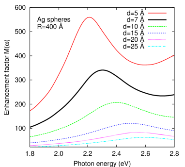
Figure 2: (color online) Calculated enhancement factors $M(\omega)$ for the incident light as a function of photon energy, for a molecule symmetrically placed between two Ag spheres with 400 Å radius. The different curves give results for a number of different molecule-particle separations $d$.

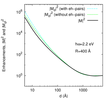
Figure 3: (color online) Calculated enhancement factors $|M|^{2}$ (full curves) and $|M_{d}|^{2}$ as a function of the molecule-particle separation $d$. As in Fig. 2, the molecule is symmetrically placed between two Ag spheres of radius 400 Å, and the photon energy is 2.2 eV. The dashed curves give $|M_{d}|^{2}$ without the contribution due to electron-hole pair creation, whereas the dash-dotted curves show $|M_{d}|^{2}$ with these contributions included.

Figures 2, 3, and 4 show calculated results related to the electromagnetic enhancement. In these calculations the molecular response which we address in more detail later plays no role, however, the placement of the molecule, i.e. where to evaluate the electric fields, is crucial. We consider a case where the molecule is placed symmetrically between the two metal nanoparticles, $d$ is the molecule-particle separation, and consequently the smallest distance between the spheres is $2d$.

Figure 2 shows results for $M(\omega,\theta=90^{\circ})$ as a function of photon energy for a few different values of $d$. There is an overall increase of the enhancement when the spheres approach each other. Moreover, the enhancement factor has a resonance peak with a resonance frequency that shifts with $d$. For $d=25$ Å it lies somewhat above 2.6 eV, but it redshifts with decreasing $d$ and for $d=5$ Å ends up at $\approx$ 2.2 eV. The resonance is caused by the interaction between the plasmon modes of the two separate spheres leading to the formation of a coupled mode with surface charges of opposite sign facing each other across the gap between the spheres. This means that a smaller $d$ gives a more charge-neutral mode, and thereby smaller restoring forces leading to the redshift shown in Fig. 2.

In Fig. 3 we have plotted the enhancement factors $|M(\omega)|^{2}$ and $|M_{d}(\omega)|^{2}$ (for the latter quantity both with and without contributions due to electron-hole pair creation) as a function of the molecule-particle separation $d$ for photon energy $\hbar\omega=2.2\mathrm{\,eV}$. Quite naturally, since $d$ spans a large range of values, so do the enhancement factors, from about 1 for $d\gtrsim 1000\mathrm{\,\r{A}}$, to $10^{5}$ or more at the smallest $d<10\mathrm{\,\r{A}}$. For distances $d$ larger than 200 Å the three curves follow each other very closely; at least on this scale no difference is discernible. This is because the silver particles are close enough to enhance the incident field and thereby, as a consequence of electromagnetic reciprocity, also enhance the radiation rate and $|M_{d}|$. But the particles are still sufficiently far away from each other and the molecule that the dielectric losses are negligible. Thus, radiation losses completely dominate other damping mechanisms here. Continuing towards smaller $d$, the two $|M_{d}|^{2}$ curves separate themselves from the $|M|^{2}$ curve because now losses in the silver particles are no longer negligible compared with radiation losses. The inclusion of damping due to electron-hole pair creation does not make any difference at first; non-local effects play no role and all loss mechanisms are already accounted for in the Mie calculation. It is only when $d$ reaches values of $\approx 30\mathrm{\,\r{A}}$ or below that the two curves representing $|M_{d}|^{2}$ with and without electron-hole pair damping begin to differ.

Figure 4: Calculated damping rates as a function of photon energy. As in Figs. 2 and 3 the molecule is symmetrically placed between two 400 Å radius silver spheres. The curves show results for three different molecule-particle separations $d$ for the separate contributions from, on one hand, electron-hole pair creation and, on the other hand, losses captured by the Mie calculations (here labeled as radiation and ohmic damping). The damping rate for the free molecule was calculated from Eq. (11) with $\ell_{\mathrm{dip}}=1$ Å.

Figure 4 shows the separate contributions to the damping rate from electron-hole pair creation and the remaining, radiative and dielectric loss mechanisms. As in the previous figure we see a rapid increase of the damping rate with decreasing $d$. This tendency is more marked for the electron-hole pair losses which vary as $1/d^{4}$. The electron-hole pair losses constitute a minor contribution for $d=20\mathrm{\,\r{A}}$, but has at $d=5\mathrm{\,\r{A}}$ become the dominant damping mechanism.

IV The molecule in free space

Given the model for the molecule discussed above, we can calculate the absorption and Raman scattering cross-sections for a molecule in free space using lowest-order perturbation theory, i.e. the Fermi golden rule.Sakurai

The absorption cross-section derived in this way reads,

$$\sigma_{A}=p_{0}^{2}\,\frac{\Omega_{L}}{c\varepsilon_{0}}\sum_{n}\frac{\hbar\Gamma_{\mathrm{tot}}\,f(0,n)f(0,n)}{(\hbar\Omega_{L}-n\hbar\omega_{\mathrm{vib}}-\hbar\Omega_{ge})^{2}+\hbar^{2}\Gamma_{\mathrm{tot}}^{2}}$$ (27)

where $\Gamma_{\mathrm{tot}}=\gamma_{ph}+\gamma_{\mathrm{vib}}/2+\gamma_{\mathrm{rad},0}/2$ and $\gamma_{\mathrm{rad},0}$ and $\gamma_{\mathrm{vib}}$ are the radiative and vibrational decay rates of the final, excited state. For the combinations of parameter values that we use, $\gamma_{ph}$ gives the completely dominating contribution to $\Gamma_{\mathrm{tot}}$ for a molecule in free space.

For the (fundamental) Raman cross-section we get in a similar way, using the Fermi golden rule with a second-order transition matrix element,

$$\sigma_{R}=p_{0}^{4}\,\frac{\omega^{\prime 3}\,\Omega_{L}}{6\pi\varepsilon_{0}^{2}c^{4}}\left|\sum_{n}\frac{f(1,n)\,f(0,n)}{\hbar\Omega_{L}-n\hbar\omega_{\mathrm{vib}}-\hbar\Omega_{ge}+i\hbar\Gamma_{\mathrm{tot}}}\right|^{2}.$$ (28)

Here $\omega^{\prime}=\Omega_{L}-\omega_{\mathrm{vib}}$, and $\Gamma_{\mathrm{tot}}=\gamma_{ph}+\gamma_{\mathrm{vib}}/2+\gamma_{\mathrm{rad},0}/2$ for the intermediate, virtual state.

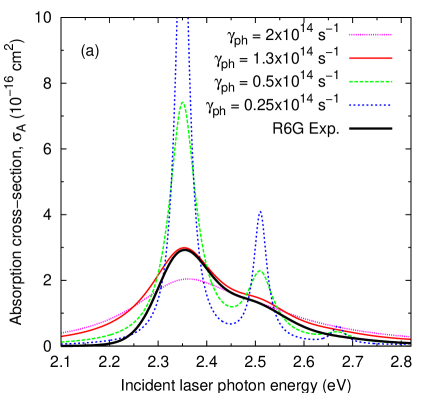
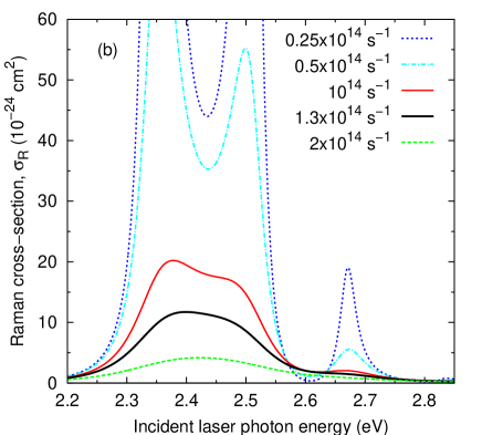
Figure 5: (color online) Calculated (a) absorption and (b) Raman profiles (i.e. cross sections as a function of incident photon energy) for a molecule in free space for a number of different dephasing rates $\gamma_{ph}$. The remaining parameter values used in the calculation are $\ell_{\mathrm{dip}}=1.2\mathrm{\,\r{A}}$, $\hbar\Omega_{ge}=2.35\mathrm{\,eV}$, $\hbar\Omega_{\mathrm{vib}}=160\mathrm{\,meV}$, and $\alpha=0.5$.

Turning to calculated results for spectra, we begin by looking at absorption and Raman profiles and their dependence on the molecular parameter values. Figure 5 shows absorption and Raman profiles plotted for a series of different dephasing rates $\gamma_{ph}$. In panel (a) we also give experimental results for the absorption cross section of a commonly used fluorescent dye molecule, Rhodamine 6G (R6G). This comparison provides some indications on what parameter values can be considered realistic. Thus we have chosen $\hbar\Omega_{ge}=2.35\mathrm{\,eV}$ to get about the same peak position in the model calculation as for R6G. The value used for $\hbar\Omega_{\mathrm{vib}}$, 160 meV, is characteristic for a C-C stretch vibration. The dipole length $\ell_{\mathrm{dip}}$ and the dephasing rate largely determine the height and width of the absorption peak. We have set $\ell_{\mathrm{dip}}=1.2\mathrm{\,\r{A}}$, while we in the calculations presented in Fig. 5 used a number of different values for $\gamma_{ph}$ to study its effects. Obviously $\gamma_{ph}=1.3\times 10^{14}\mathrm{\,s^{-1}}$ gives the best agreement with the R6G experimental spectrum; the remaining difference is the broader wings (especially on the low-frequency side) of the calculated spectrum. Finally, the Franck-Condon parameter $\alpha$ mainly determines the strength of absorption sidebands (or shoulders) due to vibrational excitations. In the calculations presented here we have used $\alpha=0.5$ and this gives a shoulder in the absorption spectrum of similar strength to that found in the R6G spectrum.

As can be seen in Fig. 5 (a), varying $\gamma_{ph}$ results in variations of the width and height of the absorption peaks; the widths are proportional to $\gamma_{ph}$ whereas the heights are approximately inversely proportional to $\gamma_{ph}$. Thus, with $\gamma_{ph}$ considerably smaller than $1.3\times 10^{14}\mathrm{\,s^{-1}}$ the vibrational sidebands create marked, resonant peaks at 2.51 eV and 2.67 eV, while with a larger $\gamma_{ph}$ the absorption spectrum is more broadened.

The Raman profiles displayed in Fig. 5 (b) show the same trends as the absorption profiles when the dephasing rate $\gamma_{ph}$ is varied, but the dependence is somewhat more complicated in this case. The Raman scattering cross section is governed by a second-order matrix element with an energy denominator with a real part set by the laser detuning and an imaginary part mainly set by $\gamma_{ph}$. Thus in the range of laser frequencies close to resonance we get peaks in the profile with a height determined by $\gamma_{ph}$. In this situation [in Fig. 5 (b) primarily between 2.3 eV and 2.5 eV] the height varies as $\sim 1/\gamma_{ph}^{2}$ and the width as $\sim\gamma_{ph}^{2}$. On the other hand, further away from resonance the detuning, not the dephasing rate, dominates the energy denominator entering the Raman scattering matrix element and in this case $\sigma_{R}$ varies much more weakly with $\gamma_{ph}$.

V Cross-section calculation

In this section we outline in detail the calculation of the spectrum of light emitted by the molecule. This includes both light scattered as a result of Rayleigh or Raman processes, and fluorescence as a result of electronic transitions in the molecule. The methods presented below makes it possible to carry out this calculations in a general case with strong enhancement of both the incident light and of the damping rate.

V.1 Emitted intensity

The emitted light intensity at the point ${\bf r}_{0}$ in the far field can be writtenScully

$$I_{\mathrm{em}}=2\varepsilon_{0}c\langle E_{\theta}^{(-)}({\bf r}_{0},t)\,E_{\theta}^{(+)}({\bf r}_{0},t)\rangle.$$ (29)

Here $E_{\theta}^{(+)}({\bf r}_{0},t)$ and $E_{\theta}^{(-)}({\bf r}_{0},t)$ stand for the positive and negative frequency parts of the $\theta$ component of the electric field, respectively. By using the normal-ordered correlation function $\langle E_{\theta}^{(-)}({\bf r}_{0},t)\,E_{\theta}^{(+)}({\bf r}_{0},t)\rangle$ we are assured that the vacuum fluctuations do not contribute to $I_{\mathrm{em}}$.

Our present goal is not only to find the total intensity of emitted light, but also its spectral distribution. Starting from Eq. (29), and using the Wiener-Khintchine theorem this can be written

$$I_{\mathrm{em}}(\omega)=\frac{1}{\pi}\mathrm{Re}\int_{0}^{\infty}d\tau\,2\varepsilon_{0}c\,\langle E_{\theta}^{(-)}({\bf r}_{0},0)\,E_{\theta}^{(+)}({\bf r}_{0},\tau)\rangle\,e^{i\omega\tau}.$$ (30)

The electric fields are caused by the electric dipole moment $p(t)$ of the molecule. A point dipole with dipole moment $\hat{z}pe^{-i\omega t}$ placed at the origin in free space generates the electric field $\vec{E}=\hat{\theta}\,p\,e^{i(kr-\omega t)}\,{\omega^{2}\sin{\theta}}/{(4\pi\varepsilon_{0}c^{2}r)}$ at a distance $r$ from the dipole. If this expression is combined with Eq. (30) we get the differential scattering and fluorescence cross-section

$$\frac{d^{2}\sigma}{d\Omega d(\hbar\omega)}=\frac{\omega^{4}\sin^{2}{\theta}}{I_{in}8\pi^{3}c^{3}\varepsilon_{0}\hbar}\mathrm{Re}\int_{0}^{\infty}d\tau\,e^{i\omega\tau}\,\langle p^{(-)}(0)\,p^{(+)}(\tau)\rangle.$$ (31)

When the molecule is no longer placed in free space the electromagnetic propagation from source to detector is modified. This can be described by the enhancement factor $M(\omega,\theta)$ introduced in Sec. III. $M(\omega,\theta)$ is closely related to a photon Green’s function.Johansson:02 The $\sin{\theta}$ factor in Eq. (31) is absorbed in $M$ which yields the emitted spectrum (in the numerical results presented below we use $\theta=90^{\circ}$ as the observation angle) from a molecule placed in the vicinity of one or several metal nanoparticles,

$$\frac{d^{2}\sigma}{d\Omega d(\hbar\omega)}=\frac{\omega^{4}|M(\omega,\theta)|^{2}}{I_{in}8\pi^{3}c^{3}\varepsilon_{0}\hbar}\mathrm{Re}\int_{0}^{\infty}d\tau\,e^{i\omega\tau}\,\langle p^{(-)}(0)\,p^{(+)}(\tau)\rangle.$$ (32)

To get any further we must evaluate the dipole-dipole correlation function $\langle p^{(-)}(0)\,p^{(+)}(\tau)\rangle$ by solving the equations of motion for the molecule dynamics. We will deal with this using density-matrix methods.

V.2 Equation of motion for the density matrix

We consider a model of the molecule with in total $N$ quantum states: two electronic levels, $|g\rangle$ and $|e\rangle$, sometimes called bands in the following, with $N_{\mathrm{vib}}$ vibrational states per electronic level, i.e. $N=2N_{\mathrm{vib}}$. The density matrix $\rho$ is thus a $2N_{\mathrm{vib}}\times 2N_{\mathrm{vib}}$ matrix with equation of motion

$$i\frac{d\rho}{dt}=\frac{1}{\hbar}[H_{\mathrm{mol}}+H^{\prime},\rho]+\mathcal{L}_{tr}\rho+\mathcal{L}_{ph}\rho.$$ (33)

The first term to the right governs the motion as a result of the molecule Hamiltonian $H_{\mathrm{mol}}$, and the interaction $H^{\prime}$, between the molecule and the laser field. The term $\mathcal{L}_{tr}\rho$ yields the damping of the density matrix as a result of transitions caused by $H_{\mathrm{fluct}}$ in which photons are spontaneously emitted, but also transitions between different vibrational levels are included in $\mathcal{L}_{tr}$ in a phenomenological way. The last term $\mathcal{L}_{ph}\rho$ makes it possible to introduce additional phase relaxation, also in a phenomenological way.

The molecular Hamiltonian is diagonal, and can be written as a sum of electronic and vibrational energies,

$$H_{mol}=\sum_{n=0}^{N_{\mathrm{vib}}-1}\sum_{l=g,e}|l;n>(E_{l}+n\hbar\Omega_{\mathrm{vib}})<l;n|.$$ (34)

To see more clearly what $H^{\prime}$ in Eq. (33) means, let us focus on a manageable example with just 4 levels ($N_{\mathrm{vib}}=2$). We then have

$$\frac{H^{\prime}}{\hbar}=\left[\begin{array}[]{cccc}0&0&V_{-}f(0,0)&V_{-}f(0,1)\\ 0&0&V_{-}f(1,0)&V_{-}f(1,1)\\ V_{+}f(0,0)&V_{+}f(1,0)&0&0\\ V_{+}f(0,1)&V_{+}f(1,1)&0&0\\ \end{array}\right],$$ (35)

and $H^{\prime}$ is explicitly time-dependent since

$$V_{\mp}=-p_{0}E_{0}e^{\pm i\Omega_{L}t}/2.$$ (36)

With these equations, and their generalizations to cases with more vibrational levels, the first term in Eq. (33) can be calculated.

Consider now the second term $\mathcal{L}_{\mathrm{tr}}\rho$, in Eq. (33). Given a spontaneous transition rate $\Gamma_{kj}$ (at zero temperature) from level $j$ to level $k$, (in our model this rate is due to vibrational damping for intraband transitions and due to radiative damping and electron-hole pair creation for interband transitions), this term can be writtenScully

$$\mathcal{L}_{tr}\rho=-\sum_{jk}\langle n_{kj}+1\rangle\frac{i\Gamma_{kj}}{2}\left[\sigma_{jk}\sigma_{kj}\rho+\rho\sigma_{jk}\sigma_{kj}-2\sigma_{kj}\rho\sigma_{jk}\right]-\sum_{jk}\langle n_{kj}\rangle\frac{i\Gamma_{kj}}{2}\left[\sigma_{kj}\sigma_{jk}\rho+\rho\sigma_{kj}\sigma_{jk}-2\sigma_{jk}\rho\sigma_{kj}\right].$$ (37)

Here $\sigma_{ab}$ stands for an operator (or matrix) with the $ab$ element equal to 1, and all the other elements equal to 0. These operators fulfill the relations

$$\sigma_{ab}\sigma_{kl}=\sigma_{al}\delta_{bk},\ \ \ \mathrm{and}\ \ \ [\sigma_{ab},\sigma_{kl}]=\sigma_{al}\delta_{bk}-\sigma_{kb}\delta_{al}.$$ (38)

The first sum in Eq. (37) refers to (possibly thermally activated) decay, the second to thermal excitation, and

$$\langle n_{kj}\rangle=1/[e^{(E_{j}-E_{k})/(k_{B}T)}-1],$$ (39)

implying that the thermal bath consists of a number of harmonic oscillators, something that is at least certainly true for the radiation damping. Given that all excitation energies $E_{j}-E_{k}$ occurring in our model are fairly large compared with $k_{B}T$, we have restricted the calculations to the zero-temperature limit, $\langle n_{kj}\rangle=0$.

The last term in the equation of motion describes dephasing of interband (i.e. ground-excited and excited-ground) coherences. This only involves one density-matrix element at a time, thus

$$\mathcal{L}_{ph}\,\rho=\mathcal{L}_{ph}\sum_{ij}\sigma_{ij}\,\rho_{ij}=-i\gamma_{ph}\sum_{i\in g}^{j\in e}(\sigma_{ij}\,\rho_{ij}+\sigma_{ji}\,\rho_{ji}),$$ (40)

where $i\in g$ indicates that when the molecule is in state $i$ it should be in the electronic ground state, etc.

V.3 Stationary state

We need to solve Eq. (33), and begin by determining the stationary-state populations and coherences. To facilitate the solution in a case with an arbitrary number of levels we form an $N^{2}$-dimensional vector $\vec{\rho}$, from the elements of the density matrix as

$$\vec{\rho}=[\rho_{11},\rho_{21},\ldots\rho_{N1},\rho_{12},\ldots\rho_{NN}].$$ (41)

The equation of motion can then be written

$$i\frac{d\vec{\rho}}{dt}=\tensor{\mathcal{L}}\vec{\rho},$$ (42)

where the tensor $\tensor{\mathcal{L}}$ describes the coupling between two density matrix elements caused by the Hamiltonian and the damping. $\tensor{\mathcal{L}}$ can be deduced from the right hand side of Eq. (33).

The stationary-state density matrix $\rho_{SS}$ is essentially time-independent, but because of the explicitly time-dependent terms in the Hamiltonian, it does have coherences (dipole moments) oscillating with the laser frequency. We therefore make the ansatz

$$\vec{\rho}_{SS}=e^{-i\tensor{\Omega}t}\vec{\rho}_{0},$$ (43)

where $\vec{\rho}_{0}$ and $\tensor{\Omega}$ are time-independent, and $\tensor{\Omega}$ is a diagonal tensor. Moreover, the diagonal elements of $\tensor{\Omega}$ referring to populations or intraband coherences equal 0. Only the diagonal elements of $\tensor{\Omega}$ referring to interband coherences are non-zero. They equal $+\Omega_{L}$, for “excited-ground” coherences and $-\Omega_{L}$ for “ground-excited” coherences. For a two-state system (just electronic degrees of freedom) we would have

$$\tensor{\Omega}=\left[\begin{array}[]{cccc}0&0&0&0\\ 0&\Omega_{L}&0&0\\ 0&0&-\Omega_{L}&0\\ 0&0&0&0\end{array}\right].$$ (44)

The stationary state can thus be determined by solving the equation

$$i\frac{d\rho_{SS}}{dt}=\tensor{\mathcal{L}}\vec{\rho}_{SS}\ \ \Leftrightarrow\ \ e^{-i\tensor{\Omega}t}\tensor{\Omega}\vec{\rho}_{0}=\tensor{\mathcal{L}}e^{-i\tensor{\Omega}t}\vec{\rho}_{0},$$ (45)

which after a multiplication by $e^{i\tensor{\Omega}t}$ can be rewritten as

$$[\tensor{\mathcal{L}}^{\prime}-\tensor{\Omega}]\vec{\rho}_{0}=0,$$ (46)

where

$$\tensor{\mathcal{L}}^{\prime}=e^{i\tensor{\Omega}t}\tensor{\mathcal{L}}e^{-i\tensor{\Omega}t}$$ (47)

is time-independent. (Basically, we have transformed the equation of motion to an interaction representation.) In addition to Eq. (46), $\rho_{0}$ must satisfy $\mathrm{Tr}[\rho_{0}]=1$.

V.4 Calculation of the spectrum

We can now focus on calculating the key quantities: the fluorescence and Rayleigh and Raman scattering cross-sections, as given by Eq. (32). The positive frequency part of the dipole operator originates from transitions from an electronically excited state to the electronic ground state. The negative frequency part, on the other hand, comes from transitions from the electronic ground state to the excited state. With the aid of the $\sigma$ operators introduced before Eq. (38) we can then write the expectation value appearing in Eq. (32),

$$\langle p^{(-)}(0)p^{(+)}(\tau)\rangle=|p_{0}|^{2}\sum_{b,k\in g}^{a,j\in e}f(b,a)f(k,j)\langle\sigma_{ab}(0)\sigma_{kj}(\tau)\rangle.$$ (48)

The expectation value $\langle\sigma_{ab}(0)\sigma_{kj}(\tau)\rangle$ can be evaluated using the quantum regression theorem (QRT), as we will show next.Scully

With the QRT the value of any element of the density matrix at time $\tau$ can be expressed as a linear combination of the density matrix elements at the earlier time $0$, provided that the process is Markovian. For a physical process to be Markovian there must not be any memory effects, damping should be frequency-independent, and the perturbing noise completely “white.” It is fairly clear that none of these conditions are fulfilled in a strict sense here, for resonant enhancement of the coupling between the molecule and the electromagnetic field implies that damping and noise is stronger at some frequencies than at others. However, the EM enhancement, see Fig. 2, varies relatively slowly, on an energy scale $\Delta E$ of a few tenths of eV, corresponding to a memory time scale $\hbar/\Delta E$ of a few femtoseconds, shorter than the other time scales relevant for the molecule dynamics. At the same time we note that in a number of interesting problems in quantum optics, for example an atom in a photonic crystal with an atomic transition energy near a band-gap edge of the photonic crystal, involves very important memory effects that require other theoretical methods and leads to novel physical phenomena.John:94 ; JackHope:01

Continuing the calculation, we first consider a one-operator expectation value and note that

$$\langle\sigma_{kj}(\tau)\rangle=\mathrm{Tr}[\rho(\tau)\sigma_{kj}]=\rho_{jk}(\tau).$$ (49)

We express this dependence through a Green’s function $G_{jk,rs}(\tau)$, thus

$$\rho_{jk}(\tau)=\sum_{rs}G_{jk,rs}(\tau)\rho_{rs}(0).$$ (50)

In the previously used vector and tensor notation this equation would read $\vec{\rho}(\tau)=\tensor{G}(\tau)\vec{\rho}(0)$. In terms of operator expectation values Eq. (50) means

$$\langle\sigma_{kj}(\tau)\rangle=\sum_{rs}G_{jk,rs}(\tau)\langle\sigma_{sr}(0)\rangle.$$ (51)

The quantum regression theoremScully states that the relation between the two-operator correlation functions $\langle\sigma_{ab}(0)\sigma_{kj}(\tau)\rangle$ and $\langle\sigma_{ab}(0)\sigma_{sr}(0)\rangle$ is identical to the one between one-operator expectation values expressed by Eq. (51), thus

$$\langle\sigma_{ab}(0)\sigma_{kj}(\tau)\rangle=\sum_{rs}G_{jk,rs}(\tau)\langle\sigma_{ab}(0)\sigma_{sr}(0)\rangle.$$ (52)

It will now be possible to calculate the dipole-moment correlation function since the expectation value appearing in Eq. (52) can be evaluated from the stationary-state density matrix $\rho_{SS}$, and the Green’s function, in view of Eq. (50), can be deduced from the equation of motion for the density matrix.

To explicitly calculate the Green’s functions we need to solve the equations of motion for the density matrix given certain initial conditions at time $t=0$, since obviously Eq. (50) states that $G_{ji,kl}(\tau)$ is the value that the element $\rho_{ji}$ will take at time $\tau$ given that all density matrix elements are 0 at time $t=0$ except the $\rho_{kl}$ which equals 1. [This should be viewed strictly mathematically; the initial conditions here sometimes mean that the density matrix is traceless and non-Hermitian. However, when $\tensor{G}$ operates on a physical $\vec{\rho}(0)$ one obtains a sensible result also for $\vec{\rho}(\tau)$.] We can thus write down an equation of motion for the Green’s tensor

$$i\frac{d\tensor{G}}{dt}-\tensor{\mathcal{L}}\tensor{G}=i\tensor{1}\delta(t),$$ (53)

where the right hand side takes care of the initial conditions [i.e. $\tensor{G}(t)\equiv 0$ for $t<0$].

To solve Eq. (53) we make an ansatz analogous to the one made for $\rho_{SS}$ above,

$$\tensor{G}(t)=e^{-i\tensor{\Omega}t}\tensor{G}_{0}(t).$$ (54)

Then by introducing the Fourier transform $\tensor{G}_{0}(\omega)$ of $\tensor{G}_{0}(t)$ through

$$\tensor{G}_{0}(\omega)=\int_{-\infty}^{\infty}dt\,e^{i\omega t}\,\tensor{G}_{0}(t),$$ (55)

we arrive at the solution

$$\tensor{G}_{0}(\omega)=i\left[(\omega+i\delta)\tensor{1}+\tensor{\Omega}-\tensor{\mathcal{L}}^{\prime}\right]^{-1}.$$ (56)

From a formal point of view the imaginary part $\delta=0$, but to avoid that the solution diverges at the driving frequency $\Omega_{L}$ we introduce a finite, but small, $\delta$. This gives a width to the calculated Rayleigh scattering peak. In the calculations reported in this paper we have used the value $\delta=2\times 10^{12}\mathrm{\,s^{-1}}$ unless otherwise stated.

We can now insert the expression for the expectation value into the equation for the cross-section,

$$\frac{d^{2}\sigma}{d\Omega d(\hbar\omega)}=\frac{\omega^{4}|M(\omega,\theta)|^{2}}{I_{in}8\pi^{3}c^{3}\varepsilon_{0}\hbar}|p_{0}|^{2}\sum_{b,k\in g}^{a,j\in e}f(b,a)\,f(k,j)\,$$

$$\times\mathrm{Re}\int_{0}^{\infty}d\tau\,e^{i\omega\tau}\sum_{rs}G_{jk,rs}(\tau)\langle\sigma_{ab}(0)\sigma_{sr}(0)\rangle.$$ (57)

The time integral gives the Green’s function Fourier transform. In view of Eq. (54) and the fact that the index $j$ refers to an excited state while $k$ refers to the electronic ground state the time integral can be written

$$\int_{0}^{\infty}d\tau\,e^{i\omega\tau}e^{-i\Omega_{L}\tau}G_{0jk,rs}(\tau)=G_{0jk,rs}(\omega-\Omega_{L}).$$ (58)

Furthermore, the expectation value can be simplified to

$$\langle\sigma_{ab}(0)\sigma_{sr}(0)\rangle=\langle\sigma_{ar}(0)\rangle\delta_{bs}=\rho_{0,ra}\delta_{bs},$$ (59)

which finally yields

$$\frac{d^{2}\sigma}{d\Omega d(\hbar\omega)}=\frac{\omega^{4}|M(\omega,\theta)|^{2}}{I_{in}8\pi^{3}c^{3}\varepsilon_{0}\hbar}|p_{0}|^{2}\sum_{b,k\in g}^{a,j\in e}f(b,a)\,f(k,j)\,$$

$$\times\sum_{r}\rho_{0,ra}\mathrm{Re}[G_{0jk,rb}(\omega-\Omega_{L})]$$ (60)

for the scattering and fluorescence cross-section.

V.5 Results in an elementary case

Equation (60) contains contributions to the cross section due to both diagonal and off-diagonal elements of the density matrix. These contributions typically have very different physical origins. The light emission related to diagonal elements are due to an excited state being populated before decaying; this describes fluorescence processes. The off-diagonal elements, on the other hand, represent an oscillating dipole moment on the molecule, and the corresponding contributions to the emitted light are due to various scattering processes.

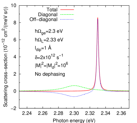
Figure 6: (color online) The spectrum of scattered light from a two-level system. In addition to showing the total cross section with a Raleigh peak as calculated from Eq. (60), the other two curves show the contributions originating from the diagonal and off-diagonal elements of the density matrix, respectively.

To illustrate this we show results for the scattering cross section in a very simple case in Fig. 6. We consider a model molecule with only two electronic levels without any sublevel structure due to vibrations (cf. Ref. Mollow, ). The electronic excitation energy is set to 2.3 eV and the incident laser photon energy is 2.33 eV. The electromagnetic enhancement is used as a parameter: both $|M|^{2}$ and $|M_{d}|^{2}$ are set to $10^{6}$, independent of the frequency $\omega$. As for damping mechanisms, we of course keep the radiation damping, but there is no dephasing in this model. By inspecting Eq. (60) we see that indices $b$, $k$, $a$, and $j$ in this case refer to one definite state (whereas they in the general case run over a set of different vibrational states), only the index $r$ can point to either the ground state or the excited state, so the cross section is a sum of two terms. The three curves in Fig. 6 show the total cross section as well as the contributions from the term proportional to the element $\rho_{0,ee}$ (diagonal) and the term proportional to $\rho_{0,ge}$ (off-diagonal). The total cross-section is everywhere positive as it should, and has a sharp peak at $\hbar\omega=2.33\mathrm{\,eV}$ due to Rayleigh scattering, (the width of this peak is set by the parameter $\delta$ used in the calculation). The Rayleigh scattering is of course the result of photons being re-emitted because the molecule has an oscillating dipole moment described by the off-diagonal elements of the density matrix, and this curve follows the one for the full cross-section closely near the laser frequency. However, for photon energies near the electron transition energy the off-diagonal contribution becomes negative, largely canceling the diagonal contributions in this case.

VI Calculated spectra

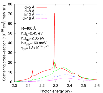
Figure 7: (color online) Calculated fluorescence and Raman spectra for a molecule placed symmetrically $d=d_{1}=d_{2}$ between two spherical ($R=400$ Å) Ag nanoparticles. Different curves correspond to different particle-molecule separations $d$. The molecule parameter values used are $\hbar\Omega_{L}=2.45$ eV, $\hbar\omega_{\mathrm{vib}}=160\mathrm{\,meV}$, $\gamma_{ph}=1.3\times 10^{14}\mathrm{\,s^{-1}}$, $\gamma_{\mathrm{vib}^{(g)}}=2\times 10^{12}\mathrm{\,s^{-1}}$, $\gamma_{\mathrm{vib}^{(e)}}=10\times 10^{12}\mathrm{\,s^{-1}}$, $\alpha=0.5$, and $I_{in}\approx 0.13\mathrm{\,\mu W/(\mu m^{2})}$.

We begin by looking at spectra calculated for a molecule placed symmetrically between two spherical Ag nanoparticles. Figure 7 displays a number of combined fluorescence and Raman spectra corresponding to different molecule-particle separations $d$, and thereby different electromagnetic enhancements. The plotted differential cross section corresponds to a situation where both the incident and scattered light propagate in the symmetry plane (i.e. $\theta=90^{\circ}$). All the spectra show a broad fluorescence background. For the smaller values of $d$, sharp Raman peaks rise above this background. The fundamental Stokes peaks, red-shifted by $\hbar\omega_{\mathrm{vib}}$ from the laser photon energy $\hbar\Omega_{L}$, are the highest ones, but at least for $d=5$ Å we can also see an overtone peak at $\hbar\Omega_{L}-2\hbar\omega_{\mathrm{vib}}$ due to creation of multiple vibrational excitations. The very strong dependence of the Raman peaks on the molecule-particle separation $d$ is the most striking tendency seen in the plot. Increasing $d$ from 5 Å to 8 Å reduces the peak height by approximately a factor of 6, at $d=12$ Å only a small Raman peak remains, and at $d=16$ Å it is nearly impossible to discern a Raman peak. The main reason for this is the stronger EM enhancement one gets with a smaller $d$, cf. Figs. 2, and 3. As was shown in Fig. 3 of Ref. Xu:04, , the Raman scattering cross section behaves as $\sigma_{R}\approx|M(\Omega_{L})|^{2}|M(\Omega-\omega_{\mathrm{vib}})|^{2}\sigma_{R,\mathrm{free}}$ as long as $d$ is not too small. The Raman cross section scales with the fourth power of the enhancement because Raman scattering involves two steps: in the first step a photon is temporarily absorbed and the molecule goes into a virtual state, in the second step a photon is emitted while the molecule goes back to the ground state, albeit to a different vibrational state. The rate of both these steps are enhanced by a factor $|M|^{2}$.

Also the fluorescence background in Fig. 7 changes with $d$; the fluorescence cross section shows an increasing tendency with decreasing $d$, however, this change is not at all as marked as for the Raman signal. Naively one may think that fluorescence, which involves an absorption event and an emission event, should also display a cross section scaling as $|M|^{4}$. But this is not so, because in the case of fluorescence the molecule is in a real, electronically excited state after having absorbed a photon but before emitting the fluorescence photon. Looking at the final step of the fluorescence process it is then clear that there are two factors that determine the fluorescence intensity: (i) the EM enhancement for the frequency of the emitted photon $|M(\omega)|^{2}$, and (ii) the probability of finding the molecule in the excited electronic state $P_{\mathrm{exc}}$. The probability $P_{\mathrm{exc}}$ is affected by the electromagnetic enhancement, but in two competing ways that largely tend to cancel each other. $P_{\mathrm{exc}}$ increases when the molecule is excited from the electronic ground state and the rate of such processes scales as $|M(\Omega_{L})|^{2}$. However, at the same time the excited state is emptied by radiative (including fluorescence) and non-radiative processes, and the rate of these is given by $|M_{d}|^{2}\gamma_{0,\mathrm{rad}}P_{\mathrm{exc}}$. Consequently, the probability of finding the molecule in an electronically excited state depends in a stationary-state situation on the EM enhancement factors as

$$P_{\mathrm{exc}}\sim|M|^{2}/|M_{d}|^{2},$$

and for the fluorescence cross section we get

$$\sigma_{F}\sim|M|^{2}P_{\mathrm{exc}}\sim|M|^{4}/|M_{d}|^{2}.$$

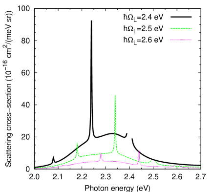
Figure 8: (color online) Calculated spectra for three different frequencies of the driving field. The molecule-particle separation is $d=5$ Å, and the rest of the parameter values are the same as in Fig. 7.

In Fig. 8 we compare three spectra calculated with different laser photon energies. These spectra result from the combined effect of a frequency-dependent Raman cross section, see Fig. 5 (b), and the frequency-dependence of the electromagnetic enhancement as shown in Fig. 2. The free-molecule Raman cross section is considerably higher for both $\hbar\Omega_{L}=2.4\mathrm{\,eV}$ and $\hbar\Omega_{L}=2.5\mathrm{\,eV}$ than for $\hbar\Omega_{L}=2.6\mathrm{\,eV}$, which explains why the Raman peak in the latter case is so small. In addition, as a result of the resonant maximum at $\approx 2.2$ eV, in Fig. 2, the combined EM enhancement $|M(\Omega_{L}-\omega_{\mathrm{vib}})|^{2}|M(\Omega_{L})|^{2}$ is the largest for $\hbar\Omega_{L}=2.4$ eV and smallest for $\hbar\Omega_{L}=2.6$ eV.

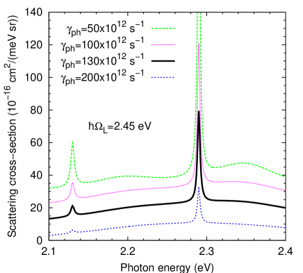
Figure 9: (color online) Calculated spectra for four different dephasing rates. The molecule-particle separation is $d=5$ Å, and the rest of the parameter values are the same as in Fig. 7. The curves have been shifted vertically for increased clarity. The truncated peak for $\gamma_{ph}=50\times 10^{12}\mathrm{\,s^{-1}}$ has height $\approx 200\times 10^{-16}\mathrm{\,cm^{2}/(meV\,sr)}$.

Figure 9 shows the spectra that result when the dephasing rate is varied. The diagram only shows the portion of the spectrum where the Raman peaks (the principal one and the first overtone) falls. Both these cross sections are, at least with a laser photon energy as close to resonance as 2.45 eV, quite sensitive to the dephasing rate. This is particularly apparent for the Raman overtone peak. For creation of multiple vibrational excitations to take place, the molecule must have a chance to “investigate” the displaced oscillator potential during a longer time than in the case of single-excitation creation. This means that the multiphonon processes are more easily disrupted when the dephasing rate goes up.

Figure 10: Calculated spectra when the molecule is placed near only one Ag particle with radius 400 Å. The molecule parameter values are the same as in Fig. 7.

In Fig. 10 we show results for a different nanoparticle configuration than the one considered so far. The results here refer to a molecule placed near only one silver particle. In this case there is some electromagnetic enhancement $M$, because the metal particle can be (resonantly) polarized. But due to the lack of electromagnetic particle-particle coupling the enhancement has a much smaller magnitude than in the two-particle case. Typically $|M|^{2}$ reaches values of 20–40 (depending on frequency) for $d=5$ Å. $M$ is less sensitive to $d$ than in the two-sphere case, the most important contribution coming from the dipole field around the particle, i.e. $|M|\sim R^{3}/(R+d)^{3}$. However, the damping rates due to losses in the particles, especially electron-hole pair creation, are still comparable to those in the two-particle case. This means that fluorescence is very strongly suppressed for small $d$ when there is only one Ag particle. For example, for $d=5$ Å a rough estimate of the ratio $|M|^{4}/|M_{d}|^{2}$ with $|M|^{2}\approx 30$ and $|M_{d}|^{2}$ taken from Fig. 3 shows that we can expect a suppression (or quenching) of the fluorescence by a factor of $\sim 10^{3}$ compared with the free-molecule case. In Fig. 10 we see in fact a difference by about 3 orders of magnitude between the fluorescence when $d$ is 5 Å and when $d$ is 1000 Å, the latter $d$ yields situation quite similar to the free-space case. For $d=5$ Å the fluorescence is suppressed to the extent that Raman peaks stand out from the background, however, the absolute Raman cross sections are of course too small to be detectable in an experiment with a single molecule.

With increasing $d$ in Fig. 10, the fluorescence yield first increases because $|M_{d}|$ decreases rapidly whereas $|M|$ falls off at a much slower rate. Then when $d$ reaches values of 50–100 Å (see the 70-Å curve) the fluorescence has a maximum, because the rate of decrease in $|M|^{4}$ overtakes that of $|M_{d}|^{2}$. For even larger $d$ $|M|^{2}\approx|M_{d}|^{2}$, so the fluorescence cross section behaves as $|M|^{2}$ there. The spectrum calculated for $d=1000$ Å approaches what one finds for the molecule in free space.

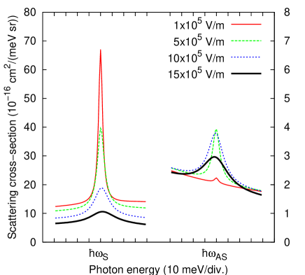
Figure 11: (color online) Calculated spectra for a molecule placed between two nanoparticles, with $d=5$ Å, for a number of different incident intensities. The other parameter values are the same as in Fig. 7. Only the energy ranges around the Raman Stokes peak at $\hbar\omega_{S}=2.29\mathrm{\,eV}$ and the Raman anti-Stokes peak at $\hbar\omega_{AS}=2.61\mathrm{\,eV}$ are shown.

The results presented so far have been calculated with moderate laser intensities. We have used the value $10^{4}\mathrm{\,V/m}$ for $E_{0}$ in Eq. (7) which corresponds to $I_{\mathrm{in}}\approx 0.13\mathrm{\,\mu W/(\mu m^{2})}$. This intensity is so low that, even in spite of the EM enhancement, the molecule spends almost all the time in the ground state (assuming, as we have done before, that thermal excitations can be neglected). The results presented in Fig. 11 (where we return to a situation with two nanoparticles) have been calculated with considerably higher incident intensities. This means that we encounter situations where there is an appreciable probability of finding the molecule electronically and/or vibrationally excited. For very strong incident fields also the response properties of the molecule changes, essentially because the probability of finding the system in a certain level becomes time-dependent (as a result of Rabi oscillations). In our calculations the stationary-state density matrices $\rho_{SS}$ and $\rho_{0}$ describe a time-average, the way the molecule “looks” on the average after long time. The dipole-dipole correlation function $\langle p^{(-)}(0)p^{(+)}(t)\rangle$, on the other hand, contains information about the molecule dynamics over a shorter period of time, starting from a certain initial state. Here Rabi oscillations due to excitation and deexcitation by a strong driving, external field show up in the results, along with other, more apparent, time-dependent aspects of the molecular dynamics such as dipole oscillations and damping.

In Fig. 11, we restrict the attention to parts of the spectra in the frequency ranges around the Stokes and anti-Stokes peaks with center frequencies $\omega_{S}=\Omega_{ge}-\omega_{\mathrm{vib}}$ and $\omega_{AS}=\Omega_{ge}+\omega_{\mathrm{vib}}$, respectively. The different spectra correspond to intensities ranging from $\approx 13\mathrm{\,\mu W/(\mu m^{2})}$ (at $E_{0}=10^{5}\mathrm{\,V/m}$) to $\approx 3.0\mathrm{\,mW/(\mu m^{2})}$ (at $E_{0}=15\times 10^{5}\mathrm{\,V/m}$). The rest of the parameter values have been chosen the same way as in the calculation behind Fig. 7. At the lowest intensity we get a Stokes peak that is nearly identical to the one in Fig. 7, but with increasing intensity the peak height diminishes quite rapidly, and it is also broadened. At the same time, at the anti-Stokes frequency, a small bump for $E_{0}=10^{5}\mathrm{\,V/m}$ develops into a marked peak at $E_{0}=5\times 10^{5}\mathrm{\,V/m}$, and subsequently also this peak is reduced in height and broadened with increasing $E_{0}$. Thus, with incident intensities of the order of $1\mathrm{\,mW/\mu m^{2}}$ it is possible to obtain anti-Stokes Raman scattering (in the model) with a cross section that is experimentally detectable. The peak values found in the figure must be multiplied by an effective peak width $\sim 10\mathrm{\,meV}$ and the effective solid angle (for dipole scattering) $8\pi/3$ to give the total Raman anti Stokes cross section. The fact that the anti-Stokes signal is weaker than the Stokes signal is here partly due to the choice of laser frequency which means that the Stokes peak falls at a maximum in the EM enhancement while the anti-Stokes peak is at a minimum for $|M|^{2}$.

To discuss the tendencies in Fig. 11 as a function of the incident field it is useful to calculate the probabilities of finding the molecule in different states. This is shown in Fig. 12. The development at moderate intensities can be well understood just from looking at the probabilities of finding the molecule in either of the two lowest states $|g\rangle|0;0\rangle$ and $|g\rangle|0;1\rangle$. With increasing intensity it becomes more likely to find the molecule in the vibrationally excited state which is a good initial state for the anti-Stokes Raman process. At the same time the vibrational ground state, the most common initial state for a Stokes Raman process, becomes more and more depopulated leading to a decreased intensity there. However, comparing the probabilities in Fig. 12 with the changes in peak heights in Fig. 11, it becomes clear that the behavior at higher intensities cannot be understood exclusively in terms of the probabilities. If this was true, the Stokes peak would not diminish as rapidly as it does, and the anti-Stokes peak would continue to increase in height. The reduced strength of both the anti-Stokes and Stokes peaks is instead the result of the molecule response becoming time-dependent at strong driving fields which leads to a smearing-out of all spectral features.

Figure 12: The probability of finding the molecule in different states and for a number of different driving fields. States numbered 0 through 5 on the horizontal axis are in the electronic ground state, i.e. $|g\rangle 0;n\rangle$ for $0\leq n\leq 5$, whereas states 6 through 11 correspond to the electronically excited states $|e\rangle x_{0};0\rangle$ through $|e\rangle x_{0};5\rangle$.

VII Discussion and Summary

We have performed a theoretical analysis of surface-enhanced Raman scattering and fluorescence based on a treatment that combines electromagnetic enhancement effects and molecule dynamics. We used a simple molecule model, however, with parameter values chosen in a realistic way.

The calculated results give Raman scattering cross sections of order $10^{-14}\mathrm{\,cm^{2}}$, thus comparable to the values found in single molecule SERS experiments,Nie:97 provided the laser frequency is reasonably close to an electronic excitation frequency of the molecule, and the electromagnetic environment (the nanoparticles) provide an EM enhancement of the Raman cross section by some 10 orders of magnitude. Thus, we conclude that the 14 to 15 orders of magnitude enhancement sometimes cited in connection with single-molecule SERS may neither be present nor needed for the effect to occur.

Our study gives an opportunity to study how the Raman and fluorescence parts of the spectra develop as the electromagnetic enhancement is varied. Most of the trends found here agree well with what one can expect compared with experiment. For the highest enhancements the Raman peaks stand out from the fluorescence background. The rather rapid decrease of the Raman cross section with increasing molecule-particle separation agrees qualitatively with results found in experiments where the metal particles are coated with a thin layer of dielectric material, the thickness of which can be controlled with reasonable precision.Bao:04 ; Cotton:98 At the same time the fluorescence background is more structured here than in most experimental results found in the literature,Nie:97 ; Xu:99 although some exceptions do exist.Weiss:01

The quenching of the fluorescence (Fig. 10) once a molecule placed near a metal surface is a well-known phenomenon, and systematic studies have also found a local maximum in the fluorescence cross section as a function of the molecule-surface distance.Kreiter:04 Compared with this study, the fluorescence maximum occurs closer to the surface in our results because of the faster drop of the electromagnetic enhancement with increasing distance from a finite nanoparticle than from a flat surface.

The model we have used in this work is a basic one containing a minimum of ingredients. To better account for some aspects of the SERS phenomenon, further developments are needed: (i) More vibrational modes should be added to better describe a fairly large organic molecule. (ii) More electronic levels could also be included. This could be a way to model “blinking” phenomena due to the molecule’s spending some time in a metastable state that is not directly optically active. One could also introduce electronic states leading to dissociation of the molecule, thus modeling photobleaching effects. (iii) Ultimately one should also try to include electron transfer processes between the molecule and the metal particles.

Appendix A Electromagnetic calculation

The coefficients $\tilde{c}$ in Eq. (21) are explicitly given by

$$\tilde{c}_{\tau\ell,m,\tau^{\prime}\ell^{\prime},m^{\prime}}(\vec{R})=\sum_{j=-1}^{1}F_{\ell m}^{j}F_{\ell^{\prime}m^{\prime}}^{j}\tilde{A}_{\ell,m+j,\ell^{\prime},m^{\prime}+j}(\vec{R}),$$ (61)

when $\tau=\tau^{\prime}$, and

$$\tilde{c}_{\tau\ell,m,\tau^{\prime}\ell^{\prime},m^{\prime}}(\vec{R})=\frac{2\ell^{\prime}+1}{i\sqrt{\ell^{\prime}(\ell^{\prime}+1)}}\,\sum_{j=-1}^{1}\mathcal{R}_{-j}\,$$

$$\times F_{\ell m}^{j}\,\tilde{A}_{\ell,m+j,\ell^{\prime}-1,m^{\prime}+j}(\vec{R})\,C_{\ell^{\prime},m^{\prime},\ell^{\prime}-1,m^{\prime}+j}^{1,-j},$$ (62)

when $\tau=\overline{\tau^{\prime}}$. In these expressions

$$F_{\ell m}^{0}=\frac{m}{\sqrt{\ell(\ell+1)}}\ \ \mathrm{and}\ \ F_{\ell m}^{\pm 1}=\frac{\sqrt{(\ell\mp m)(\ell\pm m+1)}}{\sqrt{2\ell(\ell+1)}},$$ (63)

$$\mathcal{R}_{+1}=-\sqrt{4\pi/3},\ \ \mathrm{while}\ \ \mathcal{R}_{0}=\mathcal{R}_{-1}=\sqrt{4\pi/3},$$ (64)

and the Gaunt integrals $C_{\ell,m,\ell^{\prime},m^{\prime}}^{LM}$ are defined by

$$C_{\ell,m,\ell^{\prime},m^{\prime}}^{LM}=\int d\Omega Y_{\ell m}^{*}(\Omega)Y_{LM}(\Omega)Y_{\ell^{\prime}m^{\prime}}(\Omega).$$ (65)

The coefficients $\tilde{A}$ in Eq. (61) are given by

$$\tilde{A}_{\ell,m,\ell^{\prime},m^{\prime}}(\vec{R}) =4\pi\sum_{L=|\ell-\ell^{\prime}|}^{\ell+\ell^{\prime}}(-i)^{\ell-L-\ell^{\prime}}\,h_{L}(k|\vec{R}|)$$ (66)

$$\times Y_{L,m-m^{\prime}}(\hat{R})\,C_{\ell,m,\ell^{\prime},m^{\prime}}^{L,m-m^{\prime}}.$$

Finally, the coefficients describing the external field in Eq. (13) are

$$a_{1\ell m,\mathrm{ext}}^{s}=4\pi i^{\ell}e^{i\vec{k}\cdot\vec{r}_{s}}\sum_{j=-1}^{1}Y_{\ell,m+j}^{*}(\hat{k})\,F_{\ell m}^{j}\,[\hat{e}_{j}^{*}\cdot\vec{E}_{0}],$$ (67)

and

$$a_{2\ell m,\mathrm{ext}}^{s}=4\pi i^{\ell}e^{i\vec{k}\cdot\vec{r}_{s}}\sum_{j=-1}^{1}Y_{\ell,m+j}^{*}(\hat{k})\,F_{\ell m}^{j}\,\left[\hat{e}_{j}^{*}\cdot(\hat{k}\times\vec{E}_{0})\right],$$ (68)

where the unit vectors $\hat{e}_{-1}$, $\hat{e}_{0}$, and $\hat{e}_{1}$ are given by

$$\hat{e}_{0}=\hat{z}\ \ \mathrm{and}\ \ \hat{e}_{\pm 1}=(\hat{x}\pm\hat{y}/i)/\sqrt{2},$$ (69)

and $\hat{k}=\vec{k}/|\vec{k}|$ is a unit vector in the direction of $\vec{k}$. When instead the spheres are driven by a dipole $\hat{z}p_{0}e^{-i\omega t}$ at the molecule position we have

$$a_{\tau\ell m,\mathrm{ext}}^{s}=\frac{p_{0}k^{3}}{4\pi\varepsilon_{0}}\,\sqrt{\frac{8\pi}{3}}\,\tilde{c}_{2,1,0,\tau,\ell,m}(\vec{r}_{s}).$$ (70)

Appendix B Electron-hole pair damping

In this Appendix we outline the calculation of the electron-hole pair contribution $P_{eh}/P_{\mathrm{free}}$ to the damping rate enhancement $|M_{d}|^{2}$. The non-local dielectric response of the metal particles is treated within d-parameter theory,Liebsch:87 and the derivation to a large extent follows Ref. Image, .

The idea is to model the interaction between the molecular dipole and the degrees of freedom (electron-hole pairs) of the nearby metal particles by a linear coupling between the dipole and a number of boson modes. To be specific, the dipole points along the $z$ axis and is placed at $z=h$ between two flat metal surfaces at $z=0$ and $z=L$. The interaction Hamiltonian can then be written

$$H_{int}=\sum_{\vec{q},\alpha}(C_{\vec{q},\alpha}b_{\vec{q},\alpha}+C_{\vec{q},\alpha}^{*}b_{\vec{q},\alpha}^{{\dagger}})\hat{p}.$$ (71)

Here $\hat{p}$ is the molecule dipole operator, $b$ and $b^{{\dagger}}$ are annihilation and creation operators for the bosons (with in-plane wave vector $\vec{q}$ and another branch index $\alpha$) and the coupling coefficients $C_{\vec{q},\alpha}$ are dependent on the position $h$ of the dipole. Using the Fermi golden rule, $H_{int}$ now gives a decay rate from the excited state to the ground state of the molecule which can be written

$$w=\frac{2\pi}{\hbar}|p_{0}|^{2}A\int\frac{d^{2}q}{(2\pi)^{2}}\sum_{\alpha}|C_{\vec{q},\alpha}|^{2}\delta(\hbar\Omega_{ge}-\hbar\omega_{\vec{q},\alpha}).$$ (72)

The above expression is only useful if we have a way of calculating the coefficients $C_{\vec{q},\alpha}$. To do this we evaluate the energy dissipation from a classical dipole placed at the position of the molecule to the bosonic degrees of freedom. Again, this expression will contain the coefficients $C_{\vec{q},\alpha}$, but with a classical dipole the energy dissipation rate can also be calculated using classical electrodynamics, and expressed in terms of geometric parameters and the dielectric function of the metal. We write the classical dipole moment as

$$p(t)=p_{1}(t)+p_{1}^{*}(t)=p_{1}e^{-i\omega t}+p_{1}^{*}e^{i\omega t}.$$ (73)

By letting $p(t)$ take the place of $\hat{p}$ in the Hamiltonian, we get, from the Fermi golden rule, an energy dissipation rate

$$W=2\pi\omega|p_{1}|^{2}\sum_{\vec{q},\alpha}|C_{\vec{q},\alpha}|^{2}\delta(\hbar\omega-\hbar\omega_{\vec{q},\alpha}).$$ (74)

Next we must calculate the dissipated power $W$ within the framework of classical electrodynamics. To this end we place the dipole with a dipole moment given by Eq. (73) between the metal surfaces, at $z=h$. Since all the distances involved in this calculation are very short we can ignore effects of retardation and express the solution in terms of a scalar potential $\phi(t)=\phi_{1}e^{-i\omega t}+\phi_{1}^{*}e^{i\omega t}$, where $\phi_{1}$ can be expressed as a Fourier transform

$$\phi_{1}(x,y,z)=\int\frac{d^{2}q}{(2\pi)^{2}}\tilde{\phi}_{q}(z)e^{i\vec{q}\cdot\vec{r}_{\|}},$$ (75)

($\vec{r}_{\|}=x\hat{x}+y\hat{y}$). For $\phi$ to satisfy Poisson’s equation

$$\nabla^{2}\phi=-\rho/\varepsilon_{0},$$ (76)

(where $\rho$ is the charge density due to the dipole), $\tilde{\phi}_{q}(z)$ must be a linear combination of two exponentials $e^{q_{\|}z}$ and $e^{-q_{\|}z}$. In the classical calculation we treat the surfaces in terms of their surface response functions: $g_{1}(\vec{q},\omega)$ for the surface at $z=0$ and $g_{2}(\vec{q},\omega)$ for the surface at $z=L$. The surface response function gives the negative ratio between the “reflected” potential (decaying as one leaves the surface) and the “incident” potential (decaying as one approaches the surface. Thus,

$$g(\vec{q},\omega)=-\tilde{\phi}_{q}^{\mathrm{refl}}/\tilde{\phi}_{q}^{\mathrm{inc}},$$ (77)

where the potentials should be evaluated right at the surfaces. Within d-parameter theory the surface response function is given to first order in $q_{\|}=|\vec{q}|$ asLiebsch:87

$$g(\vec{q},\omega)=\frac{\varepsilon(\omega)-1}{\varepsilon(\omega)+1}\,\left[1+\frac{\varepsilon(\omega)}{\varepsilon(\omega)+1}\,2q_{\|}d_{\perp}(\omega)\right].$$ (78)

The local dielectric function $\varepsilon(\omega)$ is the same as used in the Mie calculation and $d_{\perp}(\omega)$ is the d-parameter function. In our calculations we have evaluated $\mathrm{Im}[d_{\perp}]$ from Table I of Ref. Liebsch:87, using $r_{s}=3$ and $\hbar\omega_{p}=9\mathrm{\,eV}$ appropriate for silver in the low-frequency regime. The real part $\mathrm{Re}[d_{\perp}]$ plays a less important role; we set it to the constant value $\mathrm{Re}[d_{\perp}]=1$ Å here.

The solution for $\phi_{1}$ can now be expressed in terms of either the total incident potential at $z=0$, $\tilde{\phi}_{q,\mathrm{down}}$, as

$$\phi_{1}(x,y,z)=\int\frac{d^{2}q}{(2\pi)^{2}}e^{i\vec{q}\cdot\vec{x}}\tilde{\phi}_{q,\mathrm{down}}\left(e^{qz}-g_{1}e^{-qz}\right),$$ (79)

or, by a similar expression, in terms of $\tilde{\phi}_{q,\mathrm{up}}$, the incident potential at the upper interface. $\tilde{\phi}_{q,\mathrm{down}}$ and $\tilde{\phi}_{q,\mathrm{up}}$ are given by

$$\tilde{\phi}_{q,\mathrm{down}}=-\frac{p_{1}}{2\varepsilon_{0}}\frac{e^{-qh}+g_{2}e^{-q{(2L-h)}}}{1-g_{1}g_{2}e^{-2qL}},$$ (80)

and

$$\tilde{\phi}_{q,\mathrm{up}}=\frac{p_{1}}{2\varepsilon_{0}}\frac{e^{-q(L-h)}+g_{1}e^{-q{(L+h)}}}{1-g_{1}g_{2}e^{-2qL}}.$$ (81)

The Poynting vector $\vec{S}=\vec{E}\times\vec{H}$ at the two interfaces can here be approximated by an expression involving only $\phi$; the dissipated power is then given by

$$W=4\varepsilon_{0}\int\frac{d^{2}q}{(2\pi)^{2}}\omega q\left[|\tilde{\phi}_{q,\mathrm{down}}|^{2}\mathrm{Im}g_{1}+|\tilde{\phi}_{q,\mathrm{up}}|^{2}\mathrm{Im}g_{2}\right].$$ (82)

But this power should equal the one found in Eq. (74), and in this way we get a relation between the classical quantities found here and the sum over $\alpha$ in Eq. (74), (the sum over $q$ goes over to an integral). Inserting the so obtained expression into Eq. (72) gives

$$w=\frac{2\pi}{\hbar}|p_{0}|^{2}\int_{q_{\mathrm{min}}}^{\infty}\frac{dq_{\|}}{(2\pi)^{2}}{\varepsilon_{0}q_{\|}^{2}}\left[\left|\frac{2\tilde{\phi}_{q,\mathrm{down}}}{p_{1}}\right|^{2}\mathrm{Im}g_{1}+\left|\frac{2\tilde{\phi}_{q,\mathrm{up}}}{p_{1}}\right|^{2}\mathrm{Im}g_{2}\right].$$ (83)

The electron-hole contribution to $|M_{d}|^{2}$ in Eq. (26) can now be found as

$$P_{eh}/P_{\mathrm{free}}=w/\gamma_{\mathrm{rad},0},$$ (84)

where $\gamma_{\mathrm{rad},0}$ is found from Eq. (11) with $|f|^{2}=1$.

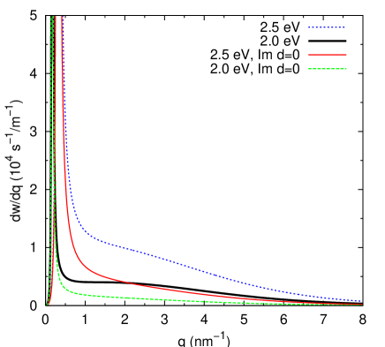
Figure 13: (color online) Plot of the function being integrated in Eq. (83).

The integrand of Eq. (83) has been plotted, for two different photon energies, as a function of $q$ in Fig. 13, both with and without a nonzero imaginary part for the function $d_{\perp}(\omega)$. This illustrates different contributions to the damping rate. At small $q$ we have damping mediated by relatively long-wavelength interactions between the molecule and the substrates. This part of the damping is actually captured by the Mie calculation discussed in the main text. In this range of $q$ space we see a fairly sharp peak around 0.5 $\mathrm{\,nm^{-1}}$ that is due to losses to a resonant interface plasmon mode formed between the two metal surfaces. We also see that the use of a non-local dielectric function, a nonzero value for $\mathrm{Im}d_{\perp}(\omega)$, has essentially no effect here. Moving towards higher $q$ values we encounter contributions to the damping that are not included in the Mie calculation. There are two reasons for this: (i) It becomes technically difficult to go to very high values for the angular momentum $\ell$ and consequently rapid (high $q$) variations of the fields are not accounted for. (ii) At these larger wave vectors the non-local effects ($\mathrm{Im}d_{\perp}(\omega)\neq 0$) that are not so easily included in the Mie calculation provides the dominant contribution to the damping. This is clearly seen in Fig. 13.

In order not to double-count contributions to the damping already included in the Mie calculation we employ a low-$q$ cutoff in Eq. (83) using $q_{\mathrm{min}}=1\mathrm{\,nm^{-1}}$. It is not really possibly to determine an exact position for the cutoff, since there is no exact correspondence between angular momenta and wave vectors, but 1 $\mathrm{\,nm^{-1}}$ is a reasonable value to use together with $R=40\mathrm{\,nm}$ and $\ell_{\mathrm{max}}=50$.

References

- (1) A. Otto, in Light Scattering in Solids IV, edited by M. Cardona and G. Guntherodt (Springer-Verlag, Berlin, 1984) p. 289.
- (2) M. Moskovits, Rev. Mod. Phys. 57, 783 (1985).
- (3) A collection of original articles can be found in Selected Papers on Surface-Enhanced Raman Scattering edited by M. Kerker (SPIE Optical Engineering Press, Bellingham, 1990).
- (4) S. Nie and S. R. Emory, Science 275, 1102 (1997).
- (5) K. Kneipp, Y. Wang, H. Kneipp, L. T. Perelman, I. Itzkan, R. R. Dasari, and M. S. Feld, Phys. Rev. Lett. 78, 1667 (1997).
- (6) H. Xu, E. J. Bjerneld, M. Käll, and L. Börjesson, Phys. Rev. Lett. 83, 4357 (1999).
- (7) A. M. Michaels, M. Nirmal, and L. E. Brus, J. Am. Chem. Soc. 121, 9932 (1999).
- (8) B. Pettinger, B. Ren, G. Picardi, R. Schuster, and G. Ertl, Phys. Rev. Lett. 92, 096101 (2004).
- (9) J. R. Lakowicz, Anal. Biochem. 298, 1 (2001).
- (10) K. Kneipp, Y. Wang, H. Kneipp, I. Itzkan, R. R. Dasari, and M. S. Feld, Phys. Rev. Lett. 76, 2444 (1996).
- (11) K. Kneipp, H. Kneipp, V. B. Kartha, R. Manoharan, G. Deinum, I. Itzkan, R. R. Dasari, and M. S. Feld, Phys. Rev. E 57, R6281 (1998).
- (12) T. L. Haslett, L. Tay, and M. Moskovits, J. Chem. Phys. 113, 1641 (2000).
- (13) A. G. Brolo, A. C. Sanderson, and A. P. Smith, Phys. Rev. B 69, 045424 (2004).
- (14) M. Moskovits, J. Chem. Phys. 69, 4159 (1978).
- (15) J. Gersten and A. Nitzan, J. Chem. Phys. 73, 3023 (1980).
- (16) T. Takemori, M. Inoue, and K. Ohtaka, J. Phys. Soc. Jpn. 56, 1587 (1987).
- (17) F. J. Garcia-Vidal and J. B. Pendry, Phys. Rev. Lett. 77, 1163 (1996).
- (18) H. X. Xu, J. Aizpurua, M. Käll, and P. Apell, Phys. Rev. E 62, 4318 (2000).
- (19) S. Corni and J. Tomasi, J. Chem. Phys. 116, 1156 (2002).
- (20) K. Li, M. I. Stockman, and D. J. Bergman, Phys. Rev. Lett. 91, 227402 (2003).
- (21) B. N. J. Persson, Chem. Phys. Lett. 82, 561 (1981).
- (22) B. Pettinger, J. Chem. Phys. 85, 7442 (1986).
- (23) A. Otto, T. Bomemann, U. Erturk, I. Mrozek, and C. Pettenkofer, Surf. Sci. 210, 363 (1989).
- (24) A. Otto, J. Raman Spectrosc. 33, 593 (2002).
- (25) H. X. Xu, X.-H. Wang, M. P. Persson, H. Q. Xu, M. Käll, and P. Johansson, Phys. Rev. Lett. 93, 243002 (2004).
- (26) Y. R. Shen, Phys. Rev. B 9, 622 (1974).
- (27) J. R. Lombardi, R. L. Birke, T. Lu, and J. Xu, J. Chem. Phys. 84, 4174 (1986).
- (28) A. Myers Kelley, J. Chem. Phys. 119, 3320 (2003).
- (29) J. D. Jackson, Classical Electrodynamics (Wiley, New York, 1975).
- (30) P. C. Waterman, Phys. Rev. D 3, 825 (1971).
- (31) E. D. Palik, Handbook of Optical Constants of Solids, (Academic Press, New York, 1985).
- (32) A. Liebsch, Phys. Rev. B 36, 7378 (1987).
- (33) W. L. Barnes, J. Mod. Opt. 45, 661 (1998).
- (34) I. A. Larkin, M. I. Stockman, M. Achermann, and V. I. Klimov, Phys. Rev. B 69, 121403 (2004).
- (35) J. J. Sakurai, Advanced Quantum Mechanics (Addison-Wesley, Reading, MA, 1967).
- (36) M. O. Scully and M. Suhail Zubairy, Quantum Optics (Cambridge University Press, Cambridge, 1997).
- (37) P. Johansson, G. Hoffmann, and R. Berndt, Phys. Rev. B 66, 245415 (2002).
- (38) S. John and T. Quang, Phys. Rev. A 50, 1764 (1994).
- (39) M. W. Jack and J. J. Hope, Phys. Rev. A 63, 043803 (2001).
- (40) B. R. Mollow, Phys. Rev. 188, 1969 (1969).
- (41) L. Bao, S. M. Mahurin, and S. Dai, Anal. Chem. 76, 4531 (2004).
- (42) K. Sokolov, G. Chumanov, and T. M. Cotton, Anal. Chem. 70, 3898 (1998).
- (43) A. Weiss and G. Haran, J. Phys. Chem. B 105, 12348.
- (44) K. Vasilev, W. Knoll, and M. Kreiter, J. Chem. Phys. 120, 3439 (2004).
- (45) B. N. J. Persson and A. Baratoff, Phys. Rev. B 38, 9616 (1988).