Host–parasite models on graphs

Abstract

The behavior of two interacting populations, “hosts” and “parasites”, is investigated on Cayley trees and scale-free networks. In the former case analytical and numerical arguments elucidate a phase diagram for the Susceptible-Infected-Susceptible model, whose most interesting feature is the absence of a tri-critical point as a function of the two independent spreading parameters. For scale-free graphs, the parasite population can be described effectively by its dynamics in a host background. This is shown both by considering the appropriate dynamical equations and by numerical simulations on Barabási-Albert networks with the major implication that in the thermodynamic limit the critical parasite spreading parameter vanishes. Some implications and generalizations are discussed.

I Introduction

Population models, or reaction-diffusion systems have attracted enormous interest both in the statistical physics community and as abstract versions of real biological dynamics. One particular aspect is the presence of phase transitions and the contact process or directed percolation in various disguises (see below, Haye ; MD ).

Host–parasite or predator–prey systems are a natural extension of single species models. By their classical results Lotka and Volterra were able to explain the nature of abundance oscillations in interacting species L ; V . In regular landscapes or lattices, with a finite spreading rate of the species, these oscillations appear as traveling waves, which can be regular or chaotic, depending on the interplay of time scales in population dynamics and spreading, though it is not clear if the phenomenon survives in the thermodynamic limit BM ; BHS ; RoA ; DA ; AD ; CHM ; HCM . In nature they have been observed in different systems, to name two extreme cases, e.g. in vole populations RK and for human diseases such as measles CHS . In the case of measles in a population living on a landscape of nontrivial island structure, power law fluctuations are found instead RA .

Much of these ideas have recently been generalized in the context of small-world or in particular “scale-free” graphs ab02 ; dmbook03 ; n03 ; pvbook04 . For the latter, a perfectly valid example is given by epidemics of viruses in the Internet since it has as a graph a fat-tailed probability distribution of the number of nearest neighbors, $P(k)$. Recently, various models have been studied as the particulars of the structure — as the so-called degree distribution gamma in $P(k)\sim k^{-\gamma}$ — are varied. A fundamental discovery concerning disease spreading is an absence of epidemic threshold in the limit of infinite graphs and the finite-size effective “critical point” obeys an unusual scaling as $L$, the graph size, is varied BA ; PSV ; ML .

This closely relates to the present work where we study the influence of a network or graph like structure of the underlying landscape on host–parasite or predator–prey dynamics. The main findings are (i) the absence of oscillations, (ii) the absence of an infection threshold in the limit of an infinite scale free graph, and (iii) the existence of two separate transitions in the case of Bethe lattices with finite coordination number $z$ (“empty” $\to$ “hosts only”, “hosts only” $\to$ “hosts plus parasites”, but no transition “empty” $\to$ “hosts plus parasites”). The structure of the rest of the paper is as follows: Section II contains the necessary definitions, and the two following ones analytical considerations and, to compare, numerical simulations of the models. Finally, Section V finishes the paper with a discussion.

II Model formulation

II.1 States and rates

A basic model for epidemiological applications is the contact process, or the so-called SIS model. Here one considers individuals living on the nodes of an underlying graph which are either infected ($I$) or susceptible ($S$) to an infection. An infected individual may spread the disease to a susceptible one if both are in contact, i.e. if they live on neighboring nodes of the graph. Infected individuals recover with a certain rate and in this simple version immediately become susceptible for a new infection. So the dynamics of the SIS model is defined by the rates

$$r_{S\to I} = \lambda\;\;\;\;\;\;\mbox{if any neighbor is infected}$$

$$r_{I\to S} = 1.$$ (1)

In this work we generalize the SIS model to a system with hosts and parasites (HP). In other words we consider infections of a second kind only able to spread onto sites with infections of first kind. So each node in the graph can be in three possible states: Empty ($e$), populated by a healthy host ($h$), or by a host with parasite ($p$). Between three states there are six possible transitions so the dynamics are defined by the following rates

$$r_{e\to h} = \lambda\;\;\;\;\;\;\mbox{if any neighbor has a host ($h$)}$$

$$r_{h\to p} = \alpha\;\mu\;\;\;\;\;\;\mbox{if any neighbor is parasitized ($p$)}$$

$$r_{h\to e} = 1$$ (2)

$$r_{e\to p} = 0$$

$$r_{p\to h} = \varepsilon$$

$$r_{p\to e} = \alpha$$

As in the SIS model defined above the decay of the host or first kind infection sets the time scale ($r_{h\to e}\!=\!1$). In biological systems $\alpha>1$ (even $\gg 1$) if the parasite affects the health of the host. A benefit would mean $\alpha<1$. We shall consider cases in which the parasite virtually does not die “on its own” but only when the host is killed, i.e. the case $0\approx\varepsilon\ll 1,\lambda,\alpha\mu,\alpha$.

Figure 1: States and rates.

In Section III we present approximate analytical solutions following PSV to the the model of Eqs. (II.1) which are compared to Monte Carlo simulations in Section IV. Particular interest lies in parasite extinction and its dependence on the parasite spreading rate $\alpha\mu$. But first we define the types of graphs used in our simulations and calculations.

II.2 Graphs

We study the population dynamics of the HP–model on two types of graphs, on Bethe lattices and on scale free Barabási–Albert (BA) graphs, in their standard version BA . A Bethe lattice of coordination number $z$ is an infinite tree, where each node has $z$ neighbors. When constructing a finite lattice, or Cayley tree, starting from a central node with $z$ neighbors and adding $z\!-\!1$ new neighbors to each boundary node, the number of boundary nodes grows exponentially. It therefore remains a finite fraction of the total number of nodes in the finite tree, which makes this construction unsuitable for Monte Carlo simulations.

This difficulty can be overcome by a slight modification DSS where a sparse homogeneous graph that closely approximates the Bethe lattice without any boundary nodes is constructed. Take $L$ nodes and label them by integers from 1 to $L$. Connect node $i$ to node $(i+1)$ for each $i$ and connect node 1 to node $L$. Construct $(z-2)$ independent random pairings of the nodes (an easy way to construct pairings is to sort the nodes randomly and pair the first node of this new order with the second one etc.) of the nodes and add an edge for each pair. By this procedure, we get a graph in which each node is of degree $z$. For large enough graphs, the loops are negligible DSS and this is a sufficient approximation of a Bethe lattice.

Here, we also use the standard version of Barabási-Albert graphs (BA-graphs) BA . These are constructed as usual. New nodes are added one by one connecting them with $m\!=\!3$ links to the previous ones. From these, the neighbors are chosen with a probability proportional to their respective number of links (preferential attachment). By this construction highly linked nodes are likely to obtain even more neighbors as the graph grows, which results in a “fat tail” distribution of probabilities for a node to have coordination number $k$, $P(k)\sim k^{-3}$ BA . The BA-graphs have very weak degree correlations, i.e. the conditional probability for a node of degree $k$ to have a neighbor with $k^{\prime}$ is rather trivial ab02 compared to many other models and real networks.

III Mean field and doublet approximation

III.1 Bethe lattice

III.1.1 Singlet (mean field) approach

In this subsection we extend the known solution for the SIS model on a Bethe lattice PSV to the HP model. $\rho_{h}$ and $\rho_{p}$ denote the density of hosts and parasites, respectively. For simplicity we consider the limit $\varepsilon=0$, so parasitized patches do not supply host individuals to neighboring empty patches. The rate equations for the densities can be written as

$$\partial_{t}\rho_{h} = -\rho_{h}+\lambda\left(1\!-\!\rho_{p}-\!\rho_{h}\right)\;\Theta-\alpha\mu\;\rho_{h}\;\Phi$$

$$\partial_{t}\rho_{p} = -\alpha\;\rho_{p}+\alpha\mu\;\rho_{h}\;\Phi$$ (3)

with $\Phi=1-(1\!-\!\rho_{p})^{z}$ and $\Theta=1-(1\!-\!\rho_{h})^{z}$.

In the absence of parasites the host population follows the dynamics of a SIS model. The trivial state $\rho_{h}=0$ is stable for $\lambda\leq 1/z$ and unstable otherwise. In other words, the host population can survive only for $\lambda>1/z$.

Similarly, the pure host phase is stable if parasites cannot invade, i.e., if the growth rate of a small parasite population is smaller than its death rate,

$$\alpha\;\mu\;z\;\rho_{h}<\alpha\;\;\;\mbox{or}\;\;\;\mu<\frac{1}{z\rho_{h}}\equiv\mu^{\rm crit}.$$ (4)

From this formula it can be seen that $\mu^{\rm crit}\to\infty$ as $\rho_{h}\to 0$, so there is no “tricritical point” in the phase plane, beyond which a direct transition from the absorbed state to the coexistence state can be seen. The phase diagram is drawn in Fig. 2.

III.1.2 Doublet approach

The singlet approach neglects occupancy correlations between adjacent nodes. The next logical step is a pair or doublet approximation which explicitly treats the joint probabilities to find two unparasitized hosts next to each other ($P_{hh}$), a healthy host next to a parasitized one ($P_{hp}$), and two parasitized next to each other ($P_{pp}$) in addition to $\rho_{h}$ and $\rho_{p}$. This approximation is widely used, we want to emphasize its application to a spatially uniform insect host–parasitoid model SMS ; OSBH , to the contact process in a one–dimensional chain MD and in general over a wide class of models BK .

The approximation uses the probabilities $P_{\sigma\sigma^{\prime}}$ to find the nodes adjacent to a randomly picked bond in states $\sigma$ and $\sigma^{\prime}\in\{e,h,p\}$, as well as the conditional probabilities $\rho_{\sigma|\sigma^{\prime}}$ to find a randomly chosen nearest neighbor of a $\sigma^{\prime}$–node in state $\sigma$. Three–point and higher correlations are neglected, so the conditional probabilities to find a $\sigma$–node next to a $\sigma^{\prime}$–node which is itself linked to a third node with state $\sigma^{\prime\prime}$ are approximated by

$$\rho_{\sigma|\sigma^{\prime}\sigma^{\prime\prime}}\approx\rho_{\sigma|\sigma^{\prime}}\;\;\;\;\;\forall\;\sigma^{\prime\prime}.$$ (5)

From there one obtains the rate equations

$$\partial_{t}\rho_{h} = \Bigl{[}-1-z\alpha\mu\rho_{p|h}+z\lambda\rho_{e|h}\Bigr{]}\;\rho_{h}$$ (6)

$$\partial_{t}\rho_{p} = \Bigl{[}-\alpha+z\alpha\mu\rho_{h|p}\Bigr{]}\;\rho_{p}$$ (7)

$$\partial_{t}P_{hh} = -\Bigl{[}2+2(z\!-\!1)\;\alpha\mu\;\rho_{p|h}\Bigr{]}\;P_{hh}$$ (8)

$$+\;\lambda\;\Bigl{[}1+(z\!-\!1)\rho_{h|e}\Bigr{]}\;P_{he}$$

$$\partial_{t}P_{hp} = -\Bigl{\{}1+\alpha+\alpha\mu\;\Bigl{[}1+(z\!-\!1)\;\rho_{p|h}\Bigr{]}\Bigr{\}}\;P_{hp}$$

$$+\;(z\!-\!1)\;\lambda\rho_{h|e}P_{pe}+2(z\!-\!1)\;\alpha\mu\rho_{p|h}P_{hh}$$

$$\partial_{t}P_{pp} = -2\alpha P_{pp}+\alpha\mu\Bigl{[}1+(z\!-\!1)\rho_{p|h}\Bigr{]}\;P_{hp}$$ (10)

$$\partial_{t}P_{he} = -\Bigl{\{}1+(z\!-\!1)\alpha\mu\rho_{p|h}$$ (11)

$$+\lambda\Bigl{[}1+(z\!-\!1)\;\rho_{h|e}\Bigr{]}\Bigr{\}}P_{he}$$

$$+2(z\!-\!1)\;\lambda\;\rho_{h|e}P_{ee}+2P_{hh}+\alpha P_{hp}$$

$$\partial_{t}P_{pe} = -\Bigl{[}\alpha+(z\!-\!1)\lambda\rho_{h|e}\Bigr{]}\;P_{pe}$$

$$+\;(z\!-\!1)\alpha\mu\;\rho_{p|h}P_{he}+P_{hp}+2\alpha P_{pp}$$

$$\partial_{t}P_{ee} = -2(z\!-\!1)\lambda\rho_{h|e}P_{ee}+P_{he}+\alpha P_{pe}$$ (13)

The joint probabilities $P_{\sigma\sigma^{\prime}}$ can be expressed in terms of the conditional probabilities as

$$P_{\sigma\sigma^{\prime}}=\rho_{\sigma}\rho_{\sigma^{\prime}|\sigma}(2-\delta_{\sigma,\sigma^{\prime}})\,,$$ (14)

where $\delta_{\sigma,\sigma^{\prime}}$ is the Kronecker symbol. The factor 2 for $\sigma\neq\sigma^{\prime}$ reflects the two possible choices, because $\sigma$ can be on either end of the bond.

There are some subtleties in Eqs. (6)–(13) that might not be immediately obvious. In Eq. (8), for instance, there is a factor of 2 in the first term. That term describes a process where an edge connecting two host–sites turns due to a death of a host into an edge connecting an empty site to a host–carrying site. The prefactor comes from the fact that this can happen in two ways, i.e. either of the the two hosts can die. For similar reasons, a prefactor of 2 can also be found in the second term of Eq. (8). However, the rest of the terms in the equation do not have these prefactors since a similar symmetry does not exist.

In principle Eqs. (6)–(13) are solvable in the steady state. Consider first the SIS model, i.e. the case without any parasites. Setting $\mu=0$ and looking at the steady-state of Eq. (6) immediately yields

$$\rho_{e|h}=\frac{1}{z\lambda}\,.$$ (15)

Similarly, setting $P_{pe}=0$ in Eq. (13) and using the identities $P_{ee}=\rho_{e}\rho_{e|e}$ and $P_{he}=2\rho_{e}\rho_{h|e}$ gives

$$\rho_{e|e}=\frac{1}{(z-1)\lambda}$$ (16)

Expressing $\rho_{h}$ as

$$\rho_{h}=\rho_{e}\frac{\rho_{h|e}}{\rho_{e|h}}=(1-\rho_{h})\frac{\rho_{h|e}}{\rho_{e|h}}\,,$$ (17)

using the identity $\rho_{e|e}+\rho_{h|e}=1$, and plugging in Eqs. (15) and (16) finally gives

$$\rho_{h}=\frac{(z-1)\lambda-1}{(z-1)\lambda-1/z}\,,$$ (18)

from the numerator of which the critical point follows:

$$\lambda_{c}^{\rm D}=\frac{1}{(z-1)}\,.$$ (19)

Note that this is different from the mean field result $\lambda_{c}^{\rm MF}=1/z$. It is also worth noting that rigorous mathematical results of the contact process P give bounds on the critical point as

$$\frac{1}{z}\leq\lambda_{c}\leq\frac{1}{z-1}\,.$$ (20)

Next consider the boundary between the parasite-absorbing and the coexistence phases. Here, hosts live well while parasites are near extinction. Expanding the steady state solution in the limit of small parasite population we derive an equation for the phase boundary: Define two auxiliary quantities $A=\rho_{h|p}$ and $B=\rho_{h|p}+\rho_{p|p}$. Form an equation for $\partial_{t}A$ and set it to vanish since we are looking at the steady-state

$$\frac{\partial A}{\partial t}\ =\frac{\partial}{\partial t}\frac{P_{hp}}{2\rho_{p}}=\frac{1}{2\rho_{p}}\left(\frac{\partial P_{hp}}{\partial t}-P_{hp}M_{p}\right)=0\,$$ (21)

where the rate equation (7) has been used, and $M_{p}$ is the Malthusian parameter or growth rate at low densities of the parasites, i.e.

$$M_{p}=-\alpha+\alpha\mu z\rho_{h|p}=-\alpha+\alpha\mu zA\,.$$ (22)

Plugging Eq. (III.1.2) into Eq. (21), using Eq. (14) and the results of Eqs. (15) and (16) at vanishing parasite population we arrive at

$$2z(z-1)(1-B)\lambda^{2}+$$

$$+\{2z^{2}\alpha\mu A(1-A)+$$

$$+2z[B-1-A(1+2\alpha\mu)]\}\lambda-$$

$$-2(z-1)A\alpha\mu = 0\,.$$ (23)

Similarly, starting at the rate equation for $B$,

$$\frac{\partial B}{\partial t}=-\frac{\partial\rho_{e|p}}{\partial t}=\frac{1}{2\rho_{p}}\left(P_{ep}M_{p}-\frac{\partial P_{ep}}{\partial t}\right)\,,$$ (24)

using Eqs. (III.1.2) and Eq. (14) together with the results of Eqs. (15) and (16), one gets

$$2z(z-1)(1-B)\lambda^{2}+$$

$$+2z^{2}\alpha\mu A(1-B)\lambda+$$

$$+2z[(B-A)(1-\alpha)-1]\lambda-$$

$$-2(z-1)A\alpha\mu = 0$$ (25)

given that $\lambda\neq 0$.

Now, solve for $A$ in the steady–state version of Eq. (7), substitute this to Eqs. (23) and (25) and eliminate $B$ from the resulting two equations to get

$$\mu=\frac{z(z-1)\lambda^{2}+z\alpha\lambda}{z(z-1)^{2}\lambda^{2}+z[(z-1)(\alpha-1)-\alpha]\lambda+\alpha(1-z)}$$ (26)

for the phase boundary between parasite-absorbing and co-existence phases in the $(\lambda,\mu)$-plane. Note that, contrary to the mean-field approximation, the phase boundary defined by this equation does not meet that defined by Eq. (19) at $\mu\to\infty$ since $\lambda=\lambda_{c}^{D}$ is not a zero of the denominator of Eq. (26). It also holds that $\mu_{c}\to 1/(z-1)$ as $\lambda\to\infty$ so that in this limit the parasites always find hosts on all nodes and therefore behave as the SIS model does.

In addition to the solution above we linearize the doublet rate equations around the previously obtained fixed point with a host population and no parasites, i.e. $\rho_{p}=P_{pp}=P_{hp}=P_{ep}=0$. Replacing the conditional probabilities $\rho_{\sigma^{\prime}|\sigma}$ by joint probabilities $P_{\sigma\sigma^{\prime}}$ as in Eq. (14) we get a matrix which is of the form

$$M=\left(\begin{array}[]{cc}M_{h}&M_{hp}\\ 0&M_{p}\end{array}\right)$$ (27)

where $M_{h}$ governs the stability of the “host only” solution, $M_{hp}$ the effect of a small parasite population on the hosts, and $M_{p}$ the growth of parasites at low densities. The block in the lower left corner is zero since the state without parasites is an absorbing one, i.e. a perturbation in the host density cannot reintroduce parasite population into the system.

The eigenvalues of a matrix with the structure of Eq. (27) are just those of $M_{h}$ and $M_{p}$, irrespective of $M_{hp}$. The stability of the host population has been discussed above, so we are only interested in the (real parts of the) eigenvalues of the matrix in the following equation,

$$\frac{d}{dt}\left(\begin{array}[]{c}\!\rho_{p}\!\\ \!P_{hp}\!\\ \!P_{pp}\!\\ \!P_{ep}\!\end{array}\right)=\left(\begin{array}[]{cccc}-\alpha&\frac{\alpha z\mu}{2}&0&0\\ 0&B&0&\tilde{\lambda}\\ 0&\alpha\mu&-2\alpha&0\\ 0&C&2\alpha&-\alpha\!-\!\tilde{\lambda}\end{array}\right)\left(\begin{array}[]{c}\!\rho_{p}\!\\ \!P_{hp}\!\\ \!P_{pp}\!\\ \!P_{ep}\!\end{array}\right)$$ (28)

with

$$B = (z\!-\!1)\alpha\mu(z\lambda\!-\!1)/(z\lambda)-1\!-\!\alpha\!-\!\alpha\mu$$ (29)

$$C = (z-1)\alpha\mu/(z\lambda)+1\;\;\mbox{and}$$ (30)

$$\tilde{\lambda} = (z-1)\lambda-1.$$ (31)

Note that $\tilde{\lambda}$ is proportional to the excess over the critical host growth rate, $\lambda-\lambda_{c}$.

The left column of the matrix in Eq. (28) is empty except for the diagonal element, which gives the first eigenvalue, $-\alpha$. We therefore restrict ourselves to the remaining $3\times 3$ matrix. It is straightforward to calculate its eigenvalues explicitly, from which the phase boundary can be deduced as follows. For each fixed $\lambda$, we consider the real part of the largest eigenvalue of the $3\times 3$ matrix as a function of $\mu$, and find its zero numerically, leading to a point $\mu(\lambda)$ that lies at the phase boundary. The results are shown in Fig. 2 for the case $\alpha=1.2$ and $z=4$.

The absence of the tricritical point can be seen easily: As $\lambda\searrow\lambda_{c}$ the excess growth rate $\tilde{\lambda}\searrow 0$, and the matrix becomes lower triangular. All three diagonal elements yield negative eigenvalues, in particular in this limit $B\to-\alpha\mu/z-\alpha-1<0$. In particular none of the eigenvalues approaches zero as $\mu\to\infty$, which leads again to the conclusion that the two phase boundaries do not meet at this limit.

In comparison to these results the mean field approximation underestimates the critical values for the spreading parameters. It does not take into account the clustering of populations, i.e., the fact that next to a populated site there is likely another one, which can not be invaded any more. So the possibility for growth is overestimated.

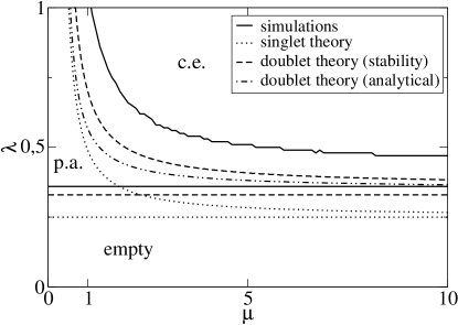
Figure 2: Phase diagram for Bethe lattice with $z=4$ in the $(\lambda,\mu)$–plane with $\alpha=1.2$ and $N=40000$ nodes. Singlet approach (mean field) compared to doublet approach (pair approximation) both analytically and via stability analysis and Monte Carlo simulations. The abbreviations denote the parasite-absorbing (p.a.), co-existence (c.e.) and empty phases, the last of which is the phase where both populations will eventually become extinct. All three solutions are in qualitative agreement with each other. As one expects, the pair approximation predicts the need of higher growth rates ($\lambda$ and $\mu$) than the singlet approach.

The phase diagram of the HP model in the $(\mu,\lambda)$-plane obtained from both theoretical approaches and from a stochastic simulation using graph approximation discussed in Sec. II.2 is drawn in Fig. 2. In the simulations, rough estimates for the phase boundaries were obtained by performing a series of simulations with different $\lambda$ for each fixed $\mu$ and observing when the population died out. The largest value of $\lambda$ at which the population dies out is then defined to be the estimate for the position of the phase boundary. From the figure we see that both analytical solutions are in qualitative agreement with each other and with the numerical results. A property worth noting of the phase diagram is the lack of a “tricritical point” and thus the phase boundary between empty and co-existence phases. Consider also that the singlet approach does reproduce the features of the phase diagram in the Bethe lattice case.

III.2 Scalefree graph

III.2.1 Singlet approach

On graphs with non-constant degrees the occupancy of a node depends on its coordination number. In general, the higher the degree of a node, the greater is its tendency to be populated. Following Ref. PSV the rate equations for the occupancies $\rho_{h}^{k}$ and $\rho_{p}^{k}$ on nodes of degree $k$ can be written as

$$\partial_{t}\rho_{h}^{k}(t) = -\rho_{h}^{k}(t)+\lambda k\left[1-\rho_{h}^{k}(t)-\rho_{p}^{k}(t)\right]\Theta_{k}(\lambda,\mu)$$ (32)

$$-\mu\alpha k\rho_{h}^{k}(t)\Phi_{k}(\lambda,\mu)$$

$$\partial_{t}\rho_{p}^{k}(t) = -\alpha\rho_{p}^{k}(t)+\mu\alpha k\rho_{h}^{k}(t)\Phi_{k}(\lambda,\mu)$$ (33)

where $\Theta_{k}(\lambda,\mu)$ and $\Phi_{k}(\lambda,\mu)$ are the probabilities that a given link points to an infected or a parasitized node, respectively. In Eq. (32) the first term on the RHS corresponds to the death of the hosts, the second one to the host spreading and the third one to parasite spreading, diminishing the number of sites that carry host but no parasite. In Eq. (33) the first term on the RHS describes the death of the parasites while the second one encompasses the spreading. It is known PSV that there is no epidemic threshold if the distribution of node degrees is fat-tailed.

The critical behavior of the HP model as obtained from the mean field equations above turns out to be incorrect and is in contradiction to the numerical findings. To see this, consider the rate equations (32) and (33) in the limit of small $\rho$, i.e. by a Taylor expansion in $\rho$. The interaction term $\mu\alpha\rho_{h}^{k}\Phi_{k}(\lambda,\mu)$ is quadratic in $\rho$ since $\Phi_{k}(\lambda,\mu)\sim\rho$ and drops out from the expansion to first order. This, in turn, means that in this limit the host population behaves as in the SIS model and the parasite population dies out since its equation only has exponentially decaying solutions. Furthermore, this rules out the possibility of a zero epidemic threshold for the parasites, since when the spreading rate approaches zero also the prevalence does so. This leads to the aforementioned contradiction. The corresponding numerical results are presented in Fig. 4.

III.2.2 Singlet approach with a substantial host population

Next, we use the singlet approach to look at the behavior of the parasites when the host population is well established. The calculation presented here is a straightforward generalization of that in Ref. BPSV .

The rate equation of the parasites in a Markovian correlated graph in the singlet approach can be written in the limit of small prevalence as

$$\frac{\partial}{\partial t}\rho_{p}^{k}=-\rho_{p}^{k}+\alpha\mu\rho_{h}^{k}\phi_{k}\,,$$ (34)

where $\phi_{k}=\sum_{k^{\prime}}k\Delta_{kk^{\prime}}\rho_{p}^{k^{\prime}}$, and $\Delta_{kk^{\prime}}=P(k^{\prime}|k)$, i.e. the conditional probability that starting from a node of degree $k$ and following a random edge one is lead to a node of degree $k^{\prime}$. For uncorrelated networks, $P(k^{\prime}|k)=kP(k^{\prime})/\langle k\rangle$, where $P(k)$ is the degree distribution of the underlying network.

If the parameters are chosen such that there are plenty of hosts and that parasites are near extinction the feedback coupling of the host population to the parasites can be neglected and $\rho_{h}^{k}$ approximated by a constant vector given by the solution of the SIS-model. The zero solution $\rho_{p}^{k}=0\,\forall k$ is always a (formal) solution of the system, so we have to study its stability. Take Eq. (34), denote $\rho=(\rho_{p}^{1}\cdots\rho_{p}^{k_{c}})^{T}$ and write the equation in a matrix form

$$\frac{\partial}{\partial t}\rho=\left(-I+\alpha\mu\rho_{h}^{k}k\Delta_{kk^{\prime}}\right)\rho=(-I+\alpha\mu C_{kk^{\prime}})\rho\,,$$ (35)

where $C_{kk^{\prime}}=\rho_{h}^{k}k\Delta_{kk^{\prime}}$.

Looking at the matrix elements $C_{kk^{\prime}}$ gives

$$C_{kk^{\prime}}\frac{P(k)}{\rho_{h}^{k}}=C_{k^{\prime}k}\frac{P(k^{\prime})}{\rho_{h}^{k^{\prime}}}\,$$ (36)

where the detailed balance condition of the network BPS

$$kP(k^{\prime}|k)P(k)=k^{\prime}P(k|k^{\prime})P(k^{\prime})$$ (37)

has been used. From Eq. (36) it follows that $C$ and $C^{T}$ have the same eigenvalues since, if $v_{k}$ is any eigenvector of $C$ corresponding to eigenvalue $\Lambda$, then $v_{k}P(k)/\rho(k)$ is an eigenvector of $C^{T}$ with the same eigenvalue. This, in turn, has the consequence that the spectrum of $C$ is real. Again, the zero solution is unstable, if the matrix $-I+\mu C$ has at least one positive eigenvalue, and the critical value of $\mu$ is $\mu_{\mathrm{critical}}=\Lambda_{M}^{-1}$.

Next, use the following corollary BPSV of the Frobenius theorem. Let $A_{kk^{\prime}}$ be any positive irreducible matrix. Its largest eigenvalue $\Lambda_{M}$ can be estimated from below as

$$\Lambda_{M}\geq\min_{k}\Bigg{\{}\frac{1}{\psi(k)}\sum_{k^{\prime}}A_{kk^{\prime}}\psi(k^{\prime})\Bigg{\}}\,,$$ (38)

where $\psi(k)$ is an arbitrary positive vector. Now, set $\psi(k)=k\rho_{h}^{k}$ and $A=C^{2}$ to get

$$\implies\Lambda_{M}\geq\min_{k}\Bigg{\{}\frac{\sum_{k^{\prime}}\sum_{l}\rho_{h}^{k}kP(l|k)\rho_{h}^{l}lP(k^{\prime}|l)k^{\prime}\rho_{h}^{k^{\prime}}}{k\rho_{h}^{k}}\Bigg{\}}$$

$$=\min_{k}\Bigg{\{}\sum_{l}l\rho_{h}^{l}P(l|k)\underbrace{\sum_{k^{\prime}}k^{\prime}\rho_{h}^{k^{\prime}}P(k^{\prime}|l)}_{=\overline{k}_{nn}^{(h)}(l,k_{c})}\Bigg{\}}\,.$$ (39)

Above $\overline{k}_{nn}^{(h)}(l,k_{c})$ denotes the average nearest neighbor degree of such neighbors that carry a host, conditioned that we are looking at a node of degree $l$. Since the average nearest neighbor degree of all neighbors $\overline{k}_{nn}(l,k_{c})=\sum_{k^{\prime}}k^{\prime}P(k^{\prime}|l)$ diverges BPSV2 as $k_{c}\to\infty$ and $\rho_{h}^{k}$ necessarily saturates to a constant value $\rho_{h}^{k=\infty}\leq 1$ with large $k$, $\overline{k}_{nn}^{(h)}(l,k_{c})$ must also diverge at the same limit. Thus the RHS of Eq. (39) diverges, giving $\Lambda_{M}\to\infty$ and

$$\mu_{\mathrm{critical}}\to 0$$ (40)

at the thermodynamic limit.

III.2.3 Doublet approach

Next, we formulate rate equations for a graph with a given degree distribution and degree-degree–correlations using the doublet approach or pair approximation. The correlations are included in the treatment since their use is natural in the context of pair approximations. The correlated network contains its uncorrelated counterpart as a special case.

The notation is as follows: $P_{\sigma\sigma^{\prime}}^{kk^{\prime}}$ is the probability that a randomly chosen edge that connects nodes with connectivities $k$ and $k^{\prime}$ is such that the state of the node with connectivity $k$ ($k^{\prime}$) is $\sigma$ ($\sigma^{\prime}$), possible states being $e$, $h$ or $p$. $Q_{\sigma\sigma^{\prime}}^{kk^{\prime}}$ is the conditional probability that a randomly chosen edge that connects nodes with connectivities $k$ and $k^{\prime}$ is such that the state of the node with connectivity $k^{\prime}$ is $\sigma^{\prime}$ conditioned that the state of the node with connectivity $k$ is $\sigma$. Let $\Delta_{kk^{\prime}}$ be as above.

Using the notation above, the rate equations for the SIS model needed for the present treatment can be written as follows

$$\partial_{t}\rho_{h}^{k} = -\rho_{h}^{k}+\lambda\sum_{k^{\prime}}k\Delta_{kk^{\prime}}P_{eh}^{kk^{\prime}}$$ (41)

$$\partial_{t}P_{hh}^{kk^{\prime}} = -2P_{hh}^{kk^{\prime}}+\lambda P_{he}^{kk^{\prime}}$$

$$+\lambda\sum_{k^{\prime\prime}}\Delta_{k^{\prime}k^{\prime\prime}}P_{he}^{k^{\prime\prime}k^{\prime}}(k^{\prime}-1)Q_{eh}^{k^{\prime}k}\,,$$

where in Eq. (III.2.3) the first term on the right hand side denotes the process where an infected node gets cured, the second the process where a node of degree $k$ infects a node of degree $k^{\prime}$ and the third the process where a node of degree $k^{\prime\prime}$ infects a node of degree $k^{\prime}$, which in turn has another neighbor of degree $k$ that is infected, turning the edge between the latter two into an edge connecting two infected nodes.

For the HP model, only one rate equation is needed for the present treatment, namely that of the parasite prevalence

$$\partial_{t}\rho_{p}^{k}=-\alpha\rho_{p}^{k}+\mu\alpha\sum_{k^{\prime}}k\Delta_{kk^{\prime}}P_{hp}^{kk^{\prime}}\,.$$ (43)

Now consider the steady-state in the SIS model. Multiply Eq. (41) by $P(k)$ and sum over all $k$ to get

$$\rho_{h}=\lambda P_{eh}\,$$ (44)

$P_{eh}$ is the fraction of all edges in the network that connect an empty node to one with host and $\rho_{h}$ is the average host prevalence in the whole network.

The last term on the right hand side of Eq. (III.2.3) is positive. Thus in the steady state we can write, leaving out the said term,

$$P_{hh}^{kk^{\prime}}\geq\frac{\lambda}{2}P_{eh}^{kk^{\prime}}\,.$$ (45)

Multiplying this by $kP(k)\Delta_{kk^{\prime}}$, summing over all $k$ and $k^{\prime}$ and combining with Eq. (44) we get

$$P_{hh}\geq\frac{1}{2}\rho_{h}\,,$$

which implies for the relative density of host–host nearest-neighbor pairs that

$$\frac{P_{hh}}{(\rho_{h})^{2}}\geq\frac{1}{2}\cdot\frac{1}{\rho_{h}}\to\infty\;\;\;\mathrm{as}\;\;\;\rho_{h}\to 0\,.$$ (46)

That is, in the limit of small population, the relative density of host–host pairs is enormous. Thus the prevalence correlations in nearest-neighbor nodes are also huge. Since the singlet approach neglects these correlations, this gives reasons to expect that it is not able to capture the properties in the HP model correctly, even though it is known that in SIS model it does BPSV .

Consider Eq. (43) in the steady state. Multiplying by $P(k)$ and summing over all $k$ gives

$$\rho_{p}=\mu P_{hp}\,$$ (47)

which in turn gives

$$\frac{P_{hp}}{\rho_{h}\rho_{p}}=\frac{1}{\mu\rho_{h}}\to\infty\;\;\;\mathrm{as}\;\;\;\rho_{p}\to 0\,,$$ (48)

since $\mu\to 0$ as $\rho_{p}\to 0$.

Eq. (47) tells that the number of edges through which the parasite population can spread is proportional to the parasite prevalence (instead of the product of parasite and host prevalences). This, in turn, tells that the dynamics of the parasites is similar to the dynamics of the hosts in the SIS model (since in the SIS model the number of edges that can spread the population is proportional to the population density in the steady-state) and serves as an explanation to the zero threshold of the parasites.

IV Monte Carlo Simulations

For a numerical comparison we have simulated the host-parasite-model in Barabási-Albert networks of sizes $L=2^{13}\ldots 2^{21}$ under the conditions in which $\rho_{h}\approx 0.30$ and $\rho_{p}\ll\rho_{h}$, i.e. with a stable hosts population and parasites close to extinction. The simulations are always started with random initial conditions by giving $25\%$ of the nodes the status $host$ and $5\%$ of the nodes the status $parasitized$ independently. Then the simulation is run for a given saturation period of $1000$ MC-steps during which even the largest system reaches a stationary state. Quantities of interest are then averaged over another $1000$ MC-steps, where one MC-step refers to the simultaneous (parallel) update event of the state variables of the nodes. The used transition probabilities $p_{\sigma\sigma^{\prime}}$ from state $\sigma$ to state $\sigma^{\prime}$ in a single time step are $p_{eh}=0.012$, $p_{he}=0.05$, $p_{pe}=0.25$ and $p_{hp}$ is varied in the range from 0.02 to 0.2 to produce the variation in $\mu=p_{hp}/p_{pe}$. This procedure was repeated $N$ times for different realizations of the graphs with $N$ varying from $N=50$ for $L=2^{13}$ to $N=5$ for $L=2^{21}$.

Fig. 3 shows how $\rho_{p}$ decays as a function of a host’s parazitation probability parameter $\mu$. Below a size dependent critical value $\mu_{c}(L)$ the parasites become extinct resulting in a left-alone host population obeying dynamics defined by the SIS-model. For instance when $L=2^{13}$ one may estimate that $\mu_{c}\approx 0.26$. The inset in the Figure 3 strongly suggests that the relationship $\rho_{p}\sim\exp(-const/\mu)$ is established as in the SIS model PSV .

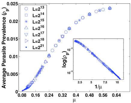
Figure 3: Average parasite prevalence as a function of its spreading parameter $\mu$. The inset corroborates an Arrhenius relation $\rho_{p}\sim\exp(-const/\mu)$, as in the SIS model PSV . The error bars are smaller than the symbol size.

To track $\mu_{c}(L)$ more accurately we have studied the extinction probability ${\cal P}_{ext}(\mu,L)$ of the parasites during $2000$ MC-steps from different realizations of BA-graphs. The critical point is then determined to be the highest value of $\mu$ below which the population dies away in a typical realization of a BA-graph, and the sizes of the error bars in $\mu_{c}$ are estimated from the width of the window in which ${\cal P}_{ext}(\mu,L)$ decays from $1$ to $0$. Fig. 4 shows a scaling $\mu_{c}(L)\sim 1/\log(L)$ in the region $2^{21}\geq L\geq 2^{16}$, which again compares to the finite size scaling of the critical threshold in the SIS model PV .

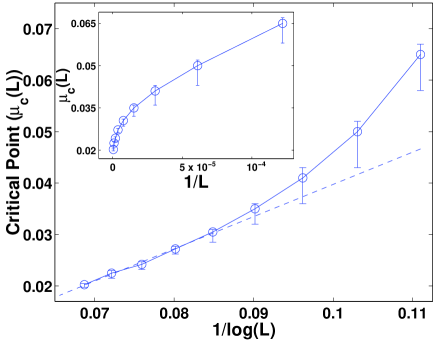
Figure 4: Scaling of the critical point vs. system size. The dashed line works as a guide to the eye and suggest $\mu_{c}(L)\sim 1/\log(L)$ as for the SIS model PSV .

Since the probability for a node to become infected depends on its degree we next take a look at the parasite prevalence of nodes of degree $k$ $\rho_{p}^{k}$ in Fig. 5 and the average degree of a site occupied by a parasite $\langle k|p\rangle$ in Fig. 6.

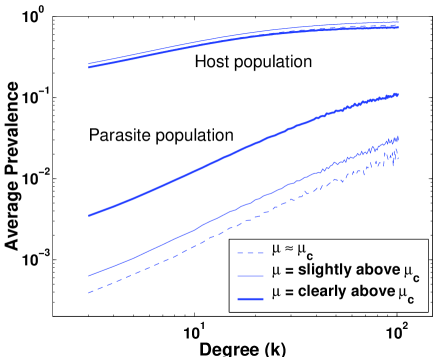
Figure 5: Average parasite prevalence and its dependence on the nodes degree. Here $L=2^{18}$ and only the $\rho_{k}$ of degree up to $k=100$ are shown since the statistics for larger $k$ become worse.

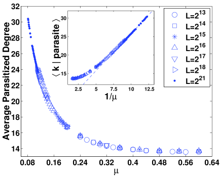
Figure 6: The expectation value of the degree of a site occupied by the parasites. A scaling form for the average degree of parasitized nodes, $\langle k|p\rangle$, is found for small $\mu$. The straight line in the inset is a guide to the eye.

Fig.  5 shows that when approaching $\mu_{c}$ the relationship $\rho_{p}^{k}\sim k$ begins to hold better and better whereas $\rho_{h}^{k}$ does not change remarkably since the host population is large. In fact, we have noted that, in analogy with the SIS-model, the scaling of $\rho_{p}^{k}$ is not just a matter of coincidence but reflects the more general presence of the factor $\rho_{p}^{k}\approx 1/(1+\mathrm{const}/k)$ which is proportional to $k$ at small $\mu$, or for large values of the constant. Generally, this behavior implies that the largest connected component of hosts serves as a “scalefree” graph for the parasites thus partly explaining the absence of a critical point in the thermodynamic limit.

As $\mu\rightarrow\mu_{c}$, survival of the parasite population becomes more and more difficult. Fig. 6 shows a consequence of this: the parasites do not prefer living in nodes of small degree anymore but, instead, the average degree of the nodes inhabited by them increases. In fact, as the inset of Fig. 6 shows, the scaling $\langle k|p\rangle\sim 1/\mu$ is established. A similar result should actually also hold for the SIS-model, and is predicted even by the mean-field equations (32) and (33). This in turn follows from the fact that for a decreasing $\alpha$ the parasite density begins to saturate only at a higher and higher $k$ (recall that it is linear in $k$ for small degrees). We have also considered the autocorrelations of the time-series of the parasite prevalence, in analogy to Ref. epjb . This decays exponentially with a time-scale constant that increases as the (pseudo–)critical point (for $L$ fixed) is approached from above.

V Discussion

In this paper we have studied a two-population model (“hosts” and “parasites”). First, as a preliminary, this problem was considered on the Bethe lattice. It turns out that the mean-field treatment can be augmented with the pair approximation. In particular we have been able to establish the generic form of phase diagram depicted in Fig. 2. This includes no tricritical point.

The main finding of this work concerns the epidemic threshold of the parasites, in the presence of a non-zero host population, on scale-free graphs. Analytical arguments based on the neighbor–pair probabilities reveal that in full analogy with the SIS model itself, the threshold is zero in the thermodynamic limit. Numerical simulations on Barabási–Albert model graphs imply that the finite-size behavior follows, also, the same scaling, and confirm this picture. These both findings might be surprising at first sight, due to the possible complications from correlations. Concomitantly, correlations in the parasite dynamics are expected to follow the same picture as in the case of the SIS model.

A striking feature related to correlated activity is the “escape” of the parasite population to vertices with, on the average, a high degree, which can actually be explained within the standard picture of (SIS-type) population behavior as the prevalence is reduced by changing a control parameter. Due to the non-regular nature of the scale-free graphs we have not seen any indications of e.g. periodic, or chaotic oscillations that arise in many similar models on regular lattices HCM ; CHM . Another possible angle would be to study contact process–like models MD , where the spreading rate out of a graph vertex to a neighbor would depend on the degree of the out-vertex, for both parasites and hosts. The phase diagram of such model would be the same for the Bethe case, but for scale-free network one would, in analogy for the contact process itself PSC , expect a finite threshold instead of the vanishing one for the SIS model. We have confirmed this, analytically, but obviously numerical studies would be of interest.

The results have implications, less for Bethe lattices which serve as an analytically tractable special case, but possibly for dynamical processes on real scale-free graphs. Examples can be found from ecology (metapopulation dynamics), where similar multi-species scenarios have already been studied. Parasitoids do play a crucial role for the population dynamics of the endangered butterfly species melitaea cinxia in its fragmented habitat on the Åland islands in the Baltic Sea, which fit less well to single species models NH ; LH . Due to the distribution of patch sizes and distances between them, the corresponding network model has a large tail degree distribution epjb . Whether a given patch is populated by hosts only or also by parasitoids depends on its local connectedness. At least qualitatively the observations agree with those in Fig. 6 and more systematic studies can be envisioned. The spreading rate depends on distance between and sizes of patches, in a nontrivial way HAM . If one translates the underlying landscape to a network model, the resulting spreading rates may depend strongly or weakly on the degree of the emitting node, i.e. lie somewhere in the range between a generalized contact process and SIS–type models. Thus the limit considered by PSC may well be relevant in certain ecological systems.

Another field of examples is epidemiology and vaccination strategies. Knowledge on non–trivial network structures in disease transmission can be used for vaccination (see e.g. OG ) or outbreak prediction, e.g. MPN , and also the importance of superinfections has been documented (see e.g. a seminal work in an evolutionary context NM ). Our ansatz is an attempt to combine both points of view. From the scale-free network viewpoint the fundamental idea of concentrating the effort on nodes with a high $k$ is valid here as well psv2 ; dalb ; consider in particular the “escape” of parasites close to extinction mentioned above. To fight parasites one needs, as well, to avoid random immunization. In this context another paradigmatic model is the “Susceptible-Infected-Removed” (SIR) model which is a variant of ordinary percolation. By taking in the HP model the right combination of limits for the parameters (essentially, disallowing recovery to the empty state from the H and P states), one obtains a variant of the SIR which resembles in such language “bootstrap percolation” since the “R” (“P”) sites are created only via contact with a neighbor in “R”. One should thus take note of possible generalizations of the HP model using similar recipes as can be applied to the SIR-style ones DW .

In the case of the SIS model, the cross-over (or the time-dependent picture) to the steady-state turns out to be interesting, which might be worth looking at here as well BBPSV . Another practical case related to this might be, say, viruses spreading as attachments to emails on the Internet NFB , where again one is confronted with a dynamical graph (of email connections) on top of a larger one (internet). Finally, we would like to point out that our work could be extended to other similar multi-species models. An example would be a hierarchy of contact processes ($A\rightarrow B$, $B\rightarrow C\dots$) THH ; GHHT .

Acknowledgments. We thank S. Zapperi and J. Lohi for stimulating discussions. An anonymous referee has brought our attention to a small but important mistake in our calculations. This work was supported by the Academy of Finland through the Centre of Excellence program (M.A., M.P., V.V.) and Deutsche Forschungsgemeinschaft via SFB 611 (M.R.). M.R. thanks Helsinki University of Technology for kind hospitality.

References

- (1) H. Hinrichsen, Adv. Phys. 49, 1, (2000).
- (2) J. Marro and R. Dickman, Nonequilibrium Phase Transitions in Lattice Models, Cambridge University Press, Cambridge (1999).
- (3) V. Volterra, Memor. Real. Accad. Naz. Lin. 2, 31 (1926).
- (4) A.J. Lotka, Elements of Physical Biology, Williams and Wilkins, Baltimore (1925).
- (5) A.T. Bradshaw and L.L. Moseley, Physica A 261, 107 (1998).
- (6) B. Blasius, A. Huppert, and L. Stone, Nature 399, 354 (1999).
- (7) A.F. Rozenfeld and E.V. Albano, Physica A 266, 322 (1999).
- (8) M. Droz and A. Pekalski, Phys. Rev. E 63, 051909 (2001).
- (9) T. Antal and M. Droz, Phys. Rev. E 63, 056119 (2001).
- (10) M.P. Hassell, H.N. Comins, and R.M. May, Nature 353, 255 (1991).
- (11) H.N. Comins, M.P. Hassell, and R.M. May, J. Anim. Ecol. 61, 735 (1992).
- (12) E. Ranta and V. Kaitala, Nature 390, 456 (1997); V. Kaitala and E. Ranta, Ecol. Lett. 1, 186 (1998).
- (13) A.D. Cliff, P. Haggett, and M. Smallman-Raynor, Measles: An Historical Geography of a Major Human Viral Disease, Blackwell, Oxford (1993).
- (14) C.J. Rhodes and R.M. Anderson, Nature 381, 600 (1996).
- (15) R. Albert and A.-L. Barabási, Rev. Mod. Phys. 74, 47 (2002).
- (16) S.N. Dorogovtsev and J.F.F. Mendes, Evolution of Networks: From Biological Nets to the Internet and WWW Oxford University Press, Oxford (2003); Adv. Phys. 51, 1079 (2002).
- (17) M.E.J. Newman, SIAM Review 45, 167 (2003).
- (18) R. Pastor-Satorras and A. Vespignani, Evolution and Structure of the Internet: A Statistical Physics Approach, Cambridge University Press, Cambridge (2004).
- (19) R. Pastor-Satorras and A. Vespignani, Phys. Rev. Lett. 86, 3200 (2001).
- (20) R.M. May and A.L. Lloyd, Phys. Rev. E 64, 066112 (2001); A.L. Lloyd and R.M. May, Science 292, 1316 (2001); A.L. Lloyd and R.M. May, Trends Ecol. Evol. 14, 417 (1999).
- (21) A.-L. Barabási and R. Albert, Science 286, 509 (1999).
- (22) D. Dhar, P. Shukla, and J.P. Sethna, J. Phys. A 45, 5259 (1997).
- (23) K. Sato, H. Matsuda, and A. Sasaki, J. Math. Biol. 32, 251 (1994).
- (24) O. Ovaskainen, K. Sato, J. Bascompte, and I. Hanski, J. Theor. Biol. 25, 95 (2002).
- (25) D. ben-Avraham and J. Köhler, Phys. Rev. A 45, 8358 (1992).
- (26) R. Pemantle, Ann. Prob. 20, 2089 (1992).
- (27) M. Boguña, R. Pastor-Satorras, and A. Vespignani, Phys. Rev. Lett. 90, 028701 (2003).
- (28) M. Boguña and R. Pastor-Satorras, Phys. Rev. E 66, 047104 (2002).
- (29) M. Boguña, R. Pastor-Satorras, and A. Vespignani, in Statistical Mechanics of Complex Networks, eds. J.M. Rubi et. al., Springer Verlag, Berlin (2003).
- (30) R. Pastor-Satorras and A. Vespignani, in Handbook of Graphs and Networks: From the Genome to the Internet, eds. S. Bornholdt and H.G. Schuster, Wiley-VCH, Berlin (2002).
- (31) R. Pastor-Satorras and C. Castellano, cond-mat/0506605.
- (32) I. Hanski, J. Alho, and A. Moilanen, Ecology 81, 239 (2000).
- (33) S. van Nouhuys and I. Hanski, J. Anim. Ecol. 71, 639 (2002).
- (34) G.C. Lei and I. Hanski, J. Anim. Ecol. 67, 422 (1998); G.C. Lei and I. Hanski, OIKOS 78, 91 (1997).
- (35) V. Vuorinen, M. Peltomäki, M. Rost, and M. Alava, Eur. Phys. J. B 38, 261 (2004).
- (36) O.T. Ovaskainen and B.T. Grenfell, Sexually Transmitted Diseases 30, 388 (2003).
- (37) L.A. Mayers, B. Pourbohloul, M.E.J. Newman, D.M. Skowronski, and R.C. Brunham, J. Theor. Biol. 232, 71 (2005).
- (38) M.A. Nowak, R.M. May, Proc. Roy. Soc. Lond. B 255, 81 (1994).
- (39) R. Pastor-Satorras and A. Vespignani, Phys. Rev. E 65, 036104 (2002).
- (40) Zoltán Dezso and A.-L. Barabási, Phys. Rev. E 65, 055103(R) (2002).
- (41) P.S. Dodds and D.J. Watts, Phys. Rev. Lett. 92, 218701 (2004).
- (42) M. Barthelemy, A. Barrat, R. Pastor-Satorras, and A. Vespignani, Phys. Rev. Lett. 92, 178701 (2004); cond-mat/0410330.
- (43) M.E.J. Newman, S. Forrest, and J. Balthrop, Phys. Rev. E 66, 035101(R) (2002).
- (44) U.C. Täuber, M. Howard, and H. Hinrichsen, Phys. Rev. Lett. 80, 2165 (1998).
- (45) Y.Y. Goldschmidt, H. Hinrichsen, M. Howard, and U.C. Täuber, Phys. Rev. E 59, 6381 (1999).