Junctions of one-dimensional quantum wires – correlation effects in transport

Abstract

We investigate transport of spinless fermions through a single site dot junction of $M$ one-dimensional quantum wires. The semi-infinite wires are described by a tight-binding model. Each wire consists of two parts: the non-interacting leads and a region of finite extent in which the fermions interact via a nearest-neighbor interaction. The functional renormalization group method is used to determine the flow of the linear conductance as a function of a low-energy cutoff for a wide range of parameters. Several fixed points are identified and their stability is analyzed. We determine the scaling exponents governing the low-energy physics close to the fixed points. Some of our results can already be derived using the non-self-consistent Hartree-Fock approximation.

I Introduction

In one spatial dimension correlation effects strongly influence the low-energy physics of many-fermion systems. Such systems cannot be described as Fermi liquids, but are classified as Tomonaga-Luttinger liquids (TLLs), which are characterized by a vanishing quasi-particle weight and power-law scaling of correlation functions.KS For spin rotationally invariant interactions and spinless fermions, on which we focus here, the exponents of the different correlation functions can be expressed in terms of a single number, the TLL parameter $K$. It depends on the parameters of the chosen model, in particular the strength of the two-particle interaction. For vanishing interaction $K=1$, while $0<K<1$ for repulsive interaction and $K>1$ in the attractive case. As indicated by the singular behavior of the density response function at momentum transfer $2k_{F}$,LutherPeschel ; Mattis with $k_{F}$ the Fermi momentum, a TLL reacts quite differently to an inhomogeneity than a Fermi liquid. The physics of inhomogeneous TLLs can conveniently be studied investigating transport properties.

The simplest junction is a single impurity in an infinite TLL wire. The transport through such a system has intensively been studied in the past. Using the renormalization group (RG) language the single impurity problem can be characterized by two fixed points (FPs).KaneFisher One is the “perfect chain” FP at which the impurity effectively vanishes and the conductance takes its maximal value. For TLL wires that are “smoothly” coupled to non-interacting leads, a situation we consider here, the latter is given by $G=e^{2}/h$.locallut The correction to the FP conductance asymptotically scales as $s^{2(K-1)}$, with $s$ being the largest (but still asymptotically small) energy scale (e.g. temperature, bias voltage, external infrared cutoff). For $0<K<1$ the exponent is negative and the FP is unstable, while it is stable for $K>1$. The other FP is the “decoupled chain” FP at which $G=0$. The correction scales as $s^{2\alpha_{B}}$, with $\alpha_{B}=1/K-1$. The FP is stable for repulsive interactions and unstable in the attractive case. The exponent $\alpha_{B}$ characterizes the power-law behavior of the local one-particle spectral weight of a TLL with an open boundary close to the boundary.KaneFisher ; FG The flow from one to the other FP is described by a $K$-dependent one-parameter scaling function. The scaling behavior of the conductance has been demonstrated for a simplified effective low-energy modelKaneFisher ; Furusaki0 ; Moon ; MatveevGlazman ; Fendley as well as for a microscopic lattice model.VM4 ; Enss04

Recently single-walled carbon nanotubes were used to experimentally realize junctions of several quasi one-dimensional quantum wires.Fuhrer ; Terrones They might form the basis of future nano-electronic devices. Taking into account the fermion interaction, models for different types of junctions and networks of TLLs have been investigated theoretically using a variety of methods.Nayak ; Safi ; Lal ; Chen ; Claudio ; Das ; Doucot ; Xavier These studies left open several interesting questions. Already the low-energy physics of the three wire Y-junction is much richer than that of the single impurity problem.

We here study the transport through a single site dot junction of $M=2,3,\ldots$ semi-infinite wires, each described by a microscopic lattice model, at temperature $T=0$. To obtain the conductance between the $M$ legs we mainly use an approximate technique that is based on the functional renormalization group (fRG) method.Wetterich ; Morris ; Manfred It has earlier been successfully applied to describe the transport in a TLL with a single impurityVM4 ; Enss04 and a double barrier,VMresotun ; Enss04 the latter allowing for resonant tunneling. The approximations lead to reliable results for not too strong interactions with TLL parameter $1/2\leq K\leq 3/2$. In particular, for a single impurity the power-law scaling of the conductance discussed above is reproduced with exponents that agree with the exact ones to leading order in the interaction. For the $M$-leg junction we investigate the RG flow for a wide range of parameters and identify the FPs. We numerically determine the exponents of the power-law corrections to the FP conductances that govern the low-energy physics close to the FPs. They depend on the interaction and the number of wires $M$. Most of these exponents have not been determined before. As in our approximation terms of second order in the interaction are only partly included the exponents can only expected to be correct to leading order in the interaction. In a short publication we have earlier verified that for a specific type of triangular three wire junction (not discussed in the present publication), for which an exact result is available,Claudio we indeed reproduce the scaling exponent to leading order.Xavier

For a specific set of junction parameters the fRG study is supplemented by results for the conductance obtained using the non-self-consistent Hartree-Fock approximation (HFA) and Fermi’s golden rule like arguments. The HFA allows us to analytically calculate one of the scaling exponents. It has earlier been shown that this approximation leads to meaningful results for the power-law scaling of the one-particle spectral weight in a TLL with an open boundary.OBCVM

The paper is organized as follows. In Sect. II we introduce our model of the $M$-wire junction. The fRG based approximation scheme is discussed in Sect. III. Using single-particle scattering theory in this section we also derive equations relating the conductance to matrix elements of an auxiliary Green function and the dot Green function. They can be used to reduce the numerical effort for solving the fRG flow equations and to gain a deeper understanding of our findings for the conductance. In Sect. IV we apply the HFA to determine scaling exponents for a certain class of symmetric junctions. Our fRG results for the FPs, the scaling exponents of the corrections to the FP conductances, and the general RG flow are presented in Sect. V. We conclude with a summary and an outlook in Sect. VI.

II The model

Each of the $M$ quantum wires that meet at that single site dot junction is described by the lattice model of spinless fermions with nearest-neighbor hopping. The semi-infinite wires can be divided in two sections: the lead with lattice sites $j>N$ in which the fermions are assumed to be non-interacting and the interacting wire with nearest-neighbor interaction across the bonds of the sites $j\in[1,N]$. Fig. 1 shows a sketch of our system. We here focus on the half-filled band case. The results are generic also for other fillings.

The Hamiltonian reads

$$H=H_{\rm kin}+H_{\rm int}+H_{\rm junc}\;.$$ (1)

The kinetic energy is modeled by

$$H_{\rm kin}=-t\,\sum_{\nu=1}^{M}\sum_{j=1}^{\infty}\big{(}\,c^{{\dagger}}_{j+1,\nu}c_{j,\nu}^{\phantom{{\dagger}}}+c^{{\dagger}}_{j,\nu}\,c_{j+1,\nu}^{\phantom{{\dagger}}}\,\big{)}$$ (2)

where we used standard second-quantized notation with $c^{{\dagger}}_{j,\nu}$ and $c_{j,\nu}^{\phantom{{\dagger}}}$ being creation and annihilation operators on site $j$ of wire $\nu$, respectively. From now on we set $t=1$, i.e. measure energies in units of $t$.

Figure 1: A single site dot junction of $M$ quantum wires. Across the bonds of the lattice sites $j=1,\ldots,N$ (small filled circles) the fermions interact via a nearest-neighbor interaction, while they are non-interacting in the leads with $j>N$ (solid line). The hopping amplitude between the first site of wire $\nu=1,\ldots,M$ and the dot site is $t_{\nu}$. The on-site energy on the dot site (large filled circle) is $V$.

As the part of the Hamiltonian containing the interaction we take

$$H_{\rm int}=\sum_{\nu=1}^{M}\sum_{j=1}^{N-1}U_{j,j+1}\left[n_{j,\nu}-1/2\right]\left[n_{j+1,\nu}-1/2\right]\;,$$ (3)

with the local density $n_{j,\nu}=c^{{\dagger}}_{j,\nu}\,c_{j,\nu}^{\phantom{{\dagger}}}$. The interaction $U_{j,j+1}$ is assumed to be independent of the wire index and acts only between the bonds of the sites $1$ to $N$, that define the interacting wire. Within this region it is allowed to depend on the position. By subtracting the average filling $1/2$ from the density $n_{j,\nu}$ we prevent a depletion of the interacting part of the wire. The chemical potential corresponding to half-filling is $\mu=0$. To avoid any fermion backscattering at the contact between the lead and the interacting wire, $U_{j,j+1}$ is turned on smoothlylocallut starting at zero across the bond $(N,N+1)$ and approaching its bulk value $U$ at bond $(N-j_{s},N-j_{s}+1)$.VM4 ; VM5 ; Enss04 More explicitly we use

$$U_{j,j+1}=\frac{U}{2}\left\{1-\frac{\arctan\left[s\;\pi(2[j-N]+j_{s})/j_{s}\right]}{\arctan[s\,\pi]}\right\}$$ (4)

for $j=N-j_{s},...,N$ and $U_{j,j+1}=U$ for $1\leq j<N-j_{s}$. The larger $N$ the smoother the interaction has to be switched on. We here consider interacting wires of up to $N=10^{5}$ sites for which $j_{s}=32$ and $s=2$ turned out to be sufficient. For these parameters the backscattering at the lead-interacting wire contact is less than $10^{-4}\%$ and can thus be neglected. The results do not dependent on the detailed shape of the envelope function as long as it is sufficiently smooth.

The model corresponding to the Hamiltonian $H_{\rm kin}+H_{\rm int}$ with interaction $U$ across all bonds (not only the ones within $[1,N]$) and $M=1$ shows TLL behavior for $|U|<2$ with a TLL parameter (for half-filling)Haldane

$$K=\left[\frac{2}{\pi}\arccos\left(-\frac{U}{2}\right)\right]^{-1}\;.$$ (5)

To leading order in the interaction it is given by

$$K=1-\frac{U}{\pi}+{\mathcal{O}}(U^{2})\;,$$ (6)

an expression we repeatedly refer to further down.

The junction we model by

$$H_{\rm junc}=-\sum_{\nu=1}^{M}t_{\nu}\big{(}\,c^{{\dagger}}_{1,\nu}d^{\phantom{{\dagger}}}+d^{{\dagger}}\,c_{1,\nu}^{\phantom{{\dagger}}}\,\big{)}+V\,d^{{\dagger}}d^{\phantom{{\dagger}}}\;,$$ (7)

with $d^{{\dagger}}$ and $d^{\phantom{{\dagger}}}$ being creation and annihilation operators on the dot site, respectively. It is parameterized by the hopping amplitudes $t_{\nu}\geq 0$ connecting the wire $\nu$ to the dot and the on-site energy $V\geq 0$ on the dot. For $M=2$ the junction is equivalent to a local impurity in an infinite wire. Applying the fRG for this case we recover the results for the conductance obtained earlier (see below).VM4 ; Enss04

Note that in our Hamilltonian the fermions on the dot site do not interact with the fermions on the first lattice sites of the wires. Including such additional interactions does not lead to any changes of the FP structure and scaling exponents investigated here, as we have verified explicitly. We exclude such terms from our model as otherwise we later would have to introduce renormalized junction parameters which would lead to an unnecessary proliferation of symbols.Enss04

III The method

At $T=0$ all inelastic processes are frozen out and the linear conductance $G_{\nu,\nu^{\prime}}$ from wire $\nu$ to wire $\nu^{\prime}$ can exactly be expressed in terms of a real space matrix element of the one-particle Green function ${\mathcal{G}}(\varepsilon+i0)$ evaluated at $\varepsilon=\mu=0$,Oguri ; Enss04

$$\frac{h}{e^{2}}\;G_{\nu,\nu^{\prime}}=\left|t_{\nu,\nu^{\prime}}\right|^{2}=4|\langle N,\nu|{\mathcal{G}}(0+i0)|N,\nu^{\prime}\rangle|^{2}\;.$$ (8)

Here $|N,\nu\rangle$ denotes the Wannier state centered on site $N$ of wire $\nu$ and $\left|t_{\nu,\nu^{\prime}}\right|^{2}$ is the effective transmission from wire $\nu$ to $\nu^{\prime}$, with $\nu\neq\nu^{\prime}$ and $\nu,\nu^{\prime}\in[1,M]$. Note that ${\mathcal{G}}(\varepsilon+i0)$ must be calculated in the presence of the non-interacting leads, the junction, and the interaction.

III.1 The functional renormalization group

To obtain an approximation for the Green function we use the fRG. A detailed account of the method was given in Refs. Enss04, and Sabine, . We here only present the approximate flow equations (which are then integrated numerically), describe the most important steps to derive them, and give details specific to the present junction geometry.

An infrared cutoff $\Lambda$ is introduced by replacing the non-interacting imaginary frequency propagator ${\mathcal{G}}_{0}$ of the system by the $\Lambda$ dependent propagator

$${\mathcal{G}}_{0}^{\Lambda}(i\omega)=\Theta(|\omega|-\Lambda)\,{\mathcal{G}}_{0}(i\omega)\;.$$ (9)

The cutoff runs from $\Lambda=\infty$ down to $\Lambda=0$, at which ${\mathcal{G}}_{0}^{\Lambda=0}(i\omega)={\mathcal{G}}_{0}(i\omega)$ is reached and the cutoff-free problem is recovered. Using the generating functional for one-particle irreducible vertex functions, with ${\mathcal{G}}_{0}^{\Lambda}$ as the non-interacting propagator, an infinite hierarchy of coupled flow equations for the self-energy, the effective two-particle interaction, and higher order vertex functions is derived.Wetterich ; Morris ; Manfred It is truncated by neglecting the three-particle vertex, which is a valid approximation as long as the two-particle vertex does not become too large. The two-particle vertex projected on the Fermi points is parameterized by an effective nearest-neighbor interaction $U^{\Lambda}$. The flow equation for the latter is obtained by considering a single infinite chain with interaction across all bonds and neglecting self-energy corrections.Sabine It can be integrated and at half-filling $U^{\Lambda}$ is given by

$$U^{\Lambda}=\frac{U}{1+\left(\Lambda-\frac{2+\Lambda^{2}}{\sqrt{4+\Lambda^{2}}}\right)\,U/(2\pi)}\;.$$ (10)

The $\Lambda$-dependent two-particle vertex is then approximated by a frequency independent nearest-neighbor interaction of strength $U^{\Lambda}$. In the case where the interaction depends on position, as an additional approximation we apply Eq. (10) locally for each bond. As a consequence of the assumed frequency independence of the effective interaction also the self-energy does not depend on $\omega$. In the exact solution an $\omega$-dependence is generated to order $U^{2}$ (bulk TLL behavior). This exemplifies that in our approximation for the self-energy terms of order $U^{2}$ are only partly included.

With these approximations the self-energy is diagonal in the wire index $\nu$ and tridiagonal in the lattice site index $j$. In a next step the non-interacting leads are projected out.Enss04 This results in an additional diagonal and Matsubara frequency $\omega$-dependent one-particle potential

$$\left<j,\nu\right|V_{\rm lead}(i\omega)\left|j^{\prime},\nu^{\prime}\right> = \frac{i\omega}{2}\left(1-\sqrt{1+\frac{4}{\omega^{2}}}\,\right)$$ (11)

$$\times\delta_{j,j^{\prime}}\,\delta_{j,N}\,\delta_{\nu,\nu^{\prime}}$$

on site $N$ of each wire $\nu$. The conductance of the infinite system Eq. (1) can then be calculated considering a finite system of $MN+1$ lattice sites.

The flow equations of the matrix elements with $j,j\pm 1\in[1,N]$ are

$$\frac{\partial}{\partial\Lambda}\Sigma^{\nu,\Lambda}_{j,j} = -\frac{1}{2\pi}\sum_{\omega=\pm\Lambda}\sum_{r=\pm 1}U^{\Lambda}_{j,j+r}$$ (12)

$$\times\left<j+r,\nu\right|{\mathcal{G}}^{\Lambda}(i\omega)\left|j+r,\nu\right>\,,$$

$$\frac{\partial}{\partial\Lambda}\Sigma^{\nu,\Lambda}_{j,j\pm 1} = \frac{U^{\Lambda}_{j,j\pm 1}}{2\pi}\sum_{\omega=\pm\Lambda}\left<j,\nu\right|{\mathcal{G}}^{\Lambda}(i\omega)\left|j\pm 1,\nu\right>\,,\;\;\;\;\;\;$$ (13)

with the propagator

$${\mathcal{G}}^{\Lambda}(i\omega)=\left[{\mathcal{G}}_{0}^{-1}(i\omega)-V_{\rm lead}(i\omega)-\Sigma^{\Lambda}\right]^{-1}\;,$$ (14)

which is a $(MN+1)\times(MN+1)$-matrix, and the initial condition

$$\Sigma^{\nu,\infty}_{j,j}=0=\Sigma^{\nu,\infty}_{j,j\pm 1}\;.$$ (15)

We introduced the notation

$$\Sigma^{\nu,\Lambda}_{j,j^{\prime}}=\left<j,\nu\right|\Sigma^{\Lambda}\left|j^{\prime},\nu\right>\;.$$

The matrix elements of the self-energy between the first sites of the wire and the dot site vanish as there is no interaction across these bonds.

In a numerical solution of Eqs. (12) and (13) the flow starts at a large finite initial cutoff $\Lambda_{0}$. One has to take into account that, due to the slow decay of the right-hand side (rhs) of the flow equation for $\Sigma^{\Lambda}$, the integration from $\Lambda=\infty$ to $\Lambda=\Lambda_{0}$ yields a contribution which does not vanish for $\Lambda_{0}\to\infty$, but rather tends to a finite constant.Sabine The resulting initial condition at $\Lambda=\Lambda_{0}\to\infty$ reads

$$\Sigma^{\nu,\Lambda_{0}}_{j,j} = \left(U_{j-1,j}+U_{j,j+1}\right)/2$$

$$\Sigma^{\nu,\Lambda_{0}}_{j,j\pm 1} = 0\;.$$ (16)

As we show in the next subsection the inversion of the $(MN+1)\times(MN+1)$-matrix on the rhs of Eqs. (12) and (13) can be reduced to the inversion of $M$ matrices of size $N\times N$.

At the end of the fRG flow the self-energy $\Sigma^{\Lambda=0}$ presents an approximation for the exact self-energy and will be denoted by $\Sigma$ in the following. In a last step to obtain the Green function ${\mathcal{G}}(z)$ which enters Eq. (8) we have to invert the matrix ${\mathcal{G}}_{0}^{-1}(z)-V_{\rm lead}(z)-\Sigma$, i.e. solve the single-particle scattering problem with $\Sigma$ and the unrenormalized junction as potentials. For $U\neq 0$, due to the fRG procedure, $\Sigma$ and thus the Green function as well as the conductance explicitly depend on the number of sites in the interacting part of the wire $N$ and the number of wires $M$. These dependences are suppressed in the notation we use. Similar to the case of a localized impurity in a single infinite wireMatveevGlazman ; VM1 ; Sabine in each wire $\nu$ the real space matrix elements $\Sigma^{\nu}_{j,j}$ and $\Sigma^{\nu}_{j,j\pm 1}$ have an important spatial dependence. They show a long-range oscillatory behavior around an average value with an amplitude which slowly decays with increasing distance from the junction. The scattering off this potential leads to the power-law scaling of the conductance.

Considering different type of geometries of inhomogeneous TLLs (single impurity, double barrier, triangular Y-junction with a magnetic flux) it was earlier shown that the above approximation scheme leads to accurate results for weak to intermediate interactions such that $1/2\leq K\leq 3/2$.VM1 ; VM5 ; VM4 ; Sabine ; VMresotun ; Enss04 ; Xavier In particular, in cases where exact expressions for scaling exponents are known from field theoretical models they are reproduced to leading order in the interaction.

Instead of analyzing the scaling of the conductance as a function of $\Lambda$ for a given set of junction parameters as well as fixed $U$ and $N$, we always integrate the flow equations down to $\Lambda=0$ and use the energy scale

$$\delta_{N}=\frac{\pi v_{F}}{N}$$ (17)

as our scaling variable. It constitutes an infrared cutoff of any power-law scaling with interaction dependent exponents.Enss04 This procedure has the advantage that each value of the scaling variable corresponds to a physical system.

III.2 Scattering theory

In this section we use single particle scattering theory to reach two goals. (i) We are aiming at an expression for the matrix elements of the $\Lambda$-dependent Green function entering the rhs of Eqs. (12) and (13) that only requires the inversion of $M$ matrices of size $N\times N$. This way the numerical effort to integrate the flow equations can considerably be reduced. (ii) Similarly to the case of resonant tunneling in a single infinite wireEnss04 we want to derive equations using Eq. (8) in which the effective transmission is expressed in terms of the diagonal matrix elements of an auxiliary Green function at site $1$ of each wire and the dot site Green function. We derive two relations of this type that will be helpful to gain a deeper understanding of our results. In the case of a symmetric junction one of them directly leads to our first result for the conductance.

The Green function ${\mathcal{G}}(z)=\left[{\mathcal{G}}_{0}^{-1}(z)-V_{\rm lead}(z)-\Sigma\right]^{-1}$ can be understood as the resolvent matrix of an effective single-particle Hamiltonian $h_{1p}(z)$ with a Hilbert space of size $NM+1$. A single-particle basis is given by the states $\{\left|j,\nu\right>,\left|d\right>\}$, where $\left|d\right>$ denotes the Wannier state centered on the dot site. The single-particle version of the junction Hamiltonian Eq. (7) is

$$h_{\rm junc}=-\sum_{\nu=1}^{M}t_{\nu}\left(\left|1,\nu\right>\left<d\right|+\mbox{H.c.}\right)+V\left|d\right>\left<d\right|\,.$$ (18)

The resolvent can be decomposed as

$${\mathcal{G}}(z)={\mathcal{G}}_{\rm dc}(z)+{\mathcal{G}}_{\rm dc}(z)h_{\rm junc}{\mathcal{G}}(z)$$ (19)

with ${\mathcal{G}}_{\rm dc}(z)$ being the resolvent of the disconnected wires

$${\mathcal{G}}_{\rm dc}(z)=\left[z-h_{1p}^{0}(z)\right]^{-1}\;.$$ (20)

The Hamiltonian $h_{1p}^{0}$ follows from $h_{1p}$ after taking $t_{\nu}=0$ for all $\nu$. Applying the projector $P=\sum_{\nu=1}^{M}P_{\nu}$ with $P_{\nu}=\sum_{j=1}^{N}|j,\nu\rangle\langle j,\nu|$, to the left and right in Eq. (19) one obtains

$$P{\mathcal{G}}(z)P = \sum_{\nu}{\mathcal{G}}^{\nu}_{\rm dc}+{\mathcal{G}}_{d}(z)$$ (21)

$$\times\sum_{\nu,\nu^{\prime}}\,t_{\nu}t_{\nu^{\prime}}{\mathcal{G}}^{\nu}_{\rm dc}(z)|1,\nu\rangle\langle 1,\nu^{\prime}|{\mathcal{G}}^{\nu^{\prime}}_{\rm dc}(z)$$

with

$${\mathcal{G}}_{d}(z)=\left[z-V-\sum_{\nu}t_{\nu}^{2}\langle 1,\nu|{\mathcal{G}}^{\nu}_{\rm dc}(z)|1,\nu\rangle\right]^{-1}$$ (22)

and

$${\mathcal{G}}^{\nu}_{\rm dc}=P_{\nu}{\mathcal{G}}_{\rm dc}(z)P_{\nu}=\left[zP_{\nu}-P_{\nu}h_{1p}^{0}(z)P_{\nu}\right]^{-1}.$$ (23)

Calculating ${\mathcal{G}}^{\nu}_{\rm dc}$ for fixed $\nu$ requires the inversion of a $N\times N$ matrix.

The steps leading to Eq. (21) can also be performed at any finite cutoff scale $\Lambda$. To determine the matrix elements of ${\mathcal{G}}^{\Lambda}$ entering the rhs of the flow equations for the self-energy (12) and (13) thus requires the knowledge of the tridiagonal parts of the inverse of $M$ tridiagonal $N\times N$-matrices $zP_{\nu}-P_{\nu}h_{1p}^{0}(z)P_{\nu}$ and a single column of each of these matrices. Numerically both can be computed in ${\mathcal{O}}(N)$ time.Sabine We can therefore easily treat a fairly large number $M$ of wires each of up to $N=10^{7}$ lattice sites with non-vanishing nearest-neighbor interaction.

Along the lines of Eqs. (19) to (24) of Ref. Enss04, it is straightforward to derive the relations

$$|t_{\nu,\nu^{\prime}}(\varepsilon)|^{2}=4\Delta_{\nu}(\varepsilon)\Delta_{\nu^{\prime}}(\varepsilon)|{\mathcal{G}}_{d}(\varepsilon+i0)|^{2}.$$ (24)

and

$$\left|t_{\nu,\nu^{\prime}}(\varepsilon)\right|^{2}=\frac{4\,\Delta_{\nu}(\varepsilon)\Delta_{\nu^{\prime}}(\varepsilon)}{\left[\varepsilon-V-\sum_{\nu^{\prime\prime}}\Omega_{\nu^{\prime\prime}}(\varepsilon)\right]^{2}+\left[\sum_{\nu^{\prime\prime}}\Delta_{\nu^{\prime\prime}}(\varepsilon)\right]^{2}}\,,$$ (25)

with real functions $\Omega_{\nu}(\varepsilon)$ and $\Delta_{\nu}(\varepsilon)$ given by

$$\Omega_{\nu}(\varepsilon)-i\Delta_{\nu}(\varepsilon)=t_{\nu}^{2}\langle 1,\nu|{\mathcal{G}}^{\nu}_{\rm dc}(\varepsilon+i0)|1,\nu\rangle\,.$$ (26)

Eqs. (24) and (25) are the expressions for the effective transmission which can be used instead of Eq. (8). Later we make extensive use of these relations.

For $V=0$ due to particle-hole symmetry $\Omega_{\nu}(0)=0$ at arbitrary $U$. If we furthermore consider a symmetric junction with $t_{1}=t_{2}=\ldots=t_{M}=\tilde{t}$ ($Z_{M}$-symmetric junction) all $\Delta_{\nu}(0)$ are equal and Eq. (25) simplifies to $\left|t_{\nu,\nu^{\prime}}(0)\right|^{2}=4/M^{2}$ independently of $U$ and $N$. The resulting conductance

$$G_{\nu,\nu^{\prime}}=\frac{e^{2}}{h}\,\frac{4}{M^{2}}\;,$$ (27)

with $\nu,\nu^{\prime}=1,\ldots,M$ and $\nu\neq\nu^{\prime}$, not only follows in the case of a junction with $\tilde{t}=1$, but for all $\tilde{t}>0$. This can be explained as a resonance phenomenon. Within our approximation scheme we thus obtained our first result for the conductance of an interacting system. As $G_{\nu,\nu^{\prime}}$ is independent of $\delta_{N}$ we identify the above case as a FP. More precisely it corresponds to a one-parameter line of FPs as the hopping $\tilde{t}$ can be varied freely. When considering this case we most of the time leave the dependence on $\tilde{t}$ implicit and refer to it as a FP. For $M$ non-interacting wires $\frac{e^{2}}{h}\,\frac{4}{M^{2}}$ is the conductance maximally allowed by the unitarity requirement of the $S$-matrix. We thus denote this FP as the “perfect junction” FP. As our approximation is correct to order $U$ we can conclude that if there is any interaction dependent correction to Eq. (27) it must be at least of order $U^{2}$.

To gain additional analytical insight we next study the one-particle spectral function for a symmetric junction of $M$ wires. From the spectral function the $\delta_{N}$-dependence of the conductance from one of the equivalent wires to an additional wire that is only weakly coupled to the junction can be deduced.

IV The Hartree-Fock approximation for symmetric junctions with $\bm{V=0}$

The one-particle spectral function $\rho_{\rm obc}$ of a TLL with an open boundary, taken at the chemical potential and close to the boundary, shows power-law scaling as a function of $\delta_{N}$ with the exponent $\alpha_{B}=1/K-1$.KaneFisher ; FG ; VM1 ; Sabine Remarkably, for $U>0$ this behavior of the spectral function can already be obtained from the non-self-consistent HFA, with a scaling exponentOBCVM

$$\alpha_{B}^{\rm HF}=\frac{U/\pi}{1+U/\pi}\;.$$ (28)

Using Eq. (6) it is straightforward to show that $\alpha_{B}^{\rm HF}$ and $\alpha_{B}$ agree to leading order in the interaction $U$. The appearance of power-law scaling within the HFA can be traced back to the spatial dependence of the self-energy. Similar to the fRG approximation of the self-energyVM1 ; Sabine the HFA self-energy shows a long-range oscillatory dependence on $j$ that implies power-law scaling of the spectral weight (see below). In contrast to the boundary problem in the single impurity problem the HFA does not reproduce the correct exponent even to leading order in $U$ as the essential RG flow of the impurity is not included.VM1 One can expect that the HFA leads to meaningful results in all models of inhomogeneous TLLs with repulsive interaction in which such a flow is unimportant. For attractive interactions the HFA can not be used even for the boundary problem as $\alpha_{B}^{\rm HF}\propto|U|>0$, while the exact exponent $\alpha_{B}$ is negative. We note in passing that for inhomogeneous TLL the application of the self-consistent HFA leads to unphysical results. As an artifact, the iteration of the Hartree-Fock equations generates a groundstate with charge-density wave order.

The above insights motivate us to study the spectral function $\rho_{1}$ on lattice site 1 (of one of the wires) for a symmetric junction of $M$ wires, with $t_{\nu}=\tilde{t}$ for $\nu=1,\ldots,M$ and $V=0$ using the HFA. We show analytically that at the chemical potential

$$\rho_{1}\propto\delta_{N}^{-\alpha^{\rm HF}_{M}}\;,$$ (29)

with a scaling exponent $\alpha^{\rm HF}_{M}$ that depends on $M$ and $U$. In the following we refer to the spectral function evaluated at the chemical potential $\mu=0$ as “the spectral weight”.

In the HFA and for $t_{\nu}=\tilde{t}$ as well as $V=0$ the Hamiltonian (1) reads

$$H_{\rm HF}= -\sum_{\nu=1}^{M}\sum_{j=1}^{\infty}t(j)\big{(}\,c^{{\dagger}}_{j+1,\nu}c_{j,\nu}^{\phantom{{\dagger}}}+c^{{\dagger}}_{j,\nu}\,c_{j+1,\nu}^{\phantom{{\dagger}}}\,\big{)}$$

$$-\tilde{t}\sum_{\nu=1}^{M}\big{(}\,c^{{\dagger}}_{1,\nu}d^{\phantom{{\dagger}}}+d^{{\dagger}}\,c_{1,\nu}^{\phantom{{\dagger}}}\,\big{)},$$ (30)

where

$$t(j)=\left\{\begin{array}[]{ll}1+U_{j,j+1}\langle c^{{\dagger}}_{j+1,\nu}c^{\phantom{{\dagger}}}_{j,\nu}\rangle_{0}&\;\mbox{for}\,1\leq j<N\\ 1&\;\mbox{otherwise}\;,\end{array}\right.$$ (33)

with the HFA self-energy $\Sigma^{\rm HF}_{j,j+1}=U_{j,j+1}\langle c^{{\dagger}}_{j+1,\nu}c^{\phantom{{\dagger}}}_{j,\nu}\rangle_{0}$. The expectation value $\langle\ldots\rangle_{0}$ is taken with the many-body groundstate of $H_{\rm kin}+H_{\rm junc}(V=0)=H_{\rm HF}(U=0)$. As we shifted the density by its average value the Hartree term vanishes.

The normalized single-particle eigenstates $|\Psi_{\varepsilon},l\rangle$ of the one-particle version $h_{\rm HF}$ of the Hartree-Fock Hamiltonian can be classified according to their behavior in $2\pi/M$-rotations ($Z_{M}$-symmetric case) which leads to the expansion

$$|\Psi_{\varepsilon},l\rangle=\delta_{l,0}a_{0}(\varepsilon)|d\rangle+\sum_{\nu=1}^{M}\sum_{j=1}^{\infty}e^{i\frac{2\pi l}{M}\nu}a_{j}^{(l)}(\varepsilon)|j,\nu\rangle\;,$$ (34)

with coefficients $a_{j}^{(l)}(\varepsilon)$ and $a_{0}(\varepsilon)$. For odd values of $M$ one has $l=0,\pm 1,\ldots,\pm(M-1)/2$, while for even values $l=0,\pm 1,\ldots,\pm M/2-1,M/2$.

IV.1 The eigenstates for $\bm{U=0}$

In a first step we determine the eigenstates of the non-interacting system. The energies are $\varepsilon=\varepsilon(k)=-2\cos(k)$. For fixed energy the wave number is thus given by $k(\varepsilon)=\arccos(-\varepsilon/2)$. Using Eq. (34)

$$h_{\rm HF}(U=0)|\Psi_{\varepsilon},l\rangle_{0}=\varepsilon|\Psi_{\varepsilon},l\rangle_{0}$$

yields

$$\varepsilon a_{j}^{(l)}(\varepsilon) = -a_{j+1}^{(l)}(\varepsilon)-a_{j-1}^{(l)}(\varepsilon)(1-\delta_{j,1})$$ (35)

$$-\tilde{t}\delta_{l,0}\delta_{j,1}a_{0}(\varepsilon)$$

for the coefficients of $|\Psi_{\varepsilon},l\rangle_{0}$. For $l=0$ there is an additional equation

$$\varepsilon a_{0}(\varepsilon)=-M\tilde{t}a_{1}^{(0)}(\varepsilon)\,.$$ (36)

The solution of Eqs. (35) and (36) is

$$a_{j}^{(l)}(\varepsilon)=A(M,\varepsilon)\sin\left\{j\,k(\varepsilon)+\delta_{l}\left[k(\varepsilon)\right]\right\}$$ (37)

and

$$a_{0}(\varepsilon)=A(M,\varepsilon)\sin\left\{\delta_{0}\left[k(\varepsilon)\right]\right\}/\tilde{t}\;,$$ (38)

with the phase shifts

$$\delta_{l}(k)=\left\{\begin{array}[]{ll}\arctan\left\{\frac{M\tilde{t}^{2}}{2-M\tilde{t}^{2}}\tan(k)\right\}&\mbox{for}\;l=0\\ 0&\mbox{otherwise}\;,\end{array}\right.$$ (41)

the normalization factor

$$A(M,\varepsilon)=\sqrt{\frac{2}{\pi\,M\,v(\varepsilon)}}\;,$$ (42)

and the velocity $v(\varepsilon)=2\left|\sin\left[k\left(\varepsilon\right)\right]\right|$.

The resulting single-particle states $|\Psi_{\varepsilon},l\rangle_{0}$ can then be used to calculate the groundstate expectation value that enters the HFA Hamiltonian

$$\langle c^{{\dagger}}_{j+1,\nu}c^{\phantom{{\dagger}}}_{j,\nu}\rangle_{0} = \sum_{l}\int_{-B/2}^{\mu}d\,\varepsilon\,a_{j+1}^{(l)}(\varepsilon)\,a_{j}^{(l)}(\varepsilon)$$ (43)

$$= \frac{1}{\pi M}\sum_{l}\int_{0}^{k_{F}}d\,k\left\{\cos[k]\right.$$

$$\left.-\cos\left[k(2j+1)+2\delta_{l}(k)\right]\right\}\;,$$

with the Fermi wave number $k_{F}=\pi/2$ and band width $B=4$. As described below to determine the scaling of the spectral weight of the interacting system for $\delta_{N}\to 0$ we only need to know the behavior of this expectation value for $1\ll j<N$

$$\langle c^{{\dagger}}_{j+1,\nu}c^{\phantom{{\dagger}}}_{j,\nu}\rangle_{0}=\frac{1}{\pi}\left[1-\frac{(-1)^{j}}{2j+1}\left(1-\frac{2}{M}\right)+{\mathcal{O}}\left(j^{-2}\right)\right].$$

This asymptotic behavior can be obtained from Eq. (43) using integration by parts and $\delta_{0}(k_{F})=\pm\pi/2$. For $1\leq j\leq N-j_{s}$ the interaction $U_{j,j+1}$ Eq. (4) takes its bulk value $U$ and it follows that

$$t(j) = 1+\frac{U}{\pi}-\frac{U}{\pi}\frac{(-1)^{j}}{2j+1}\left(1-\frac{2}{M}\right)$$ (44)

$$= \left(1+\frac{U}{\pi}\right)\left[1-\alpha_{B}^{\rm HF}\frac{(-1)^{j}}{2j+1}\left(1-\frac{2}{M}\right)\right]\;,$$

for $1\ll j\leq N-j_{s}$.

IV.2 Spectral weight for $\bm{U\neq 0}$

Within the HFA the spectral weight on the first site of one of the equivalent legs is determined by the amplitudes of the $\varepsilon=0$ eigenstates $|\Psi_{\varepsilon=0},l\rangle$ of $h_{\rm HF}$

$$\rho_{1}\propto\sum_{l}\left|\left<1,\nu\right.|\Psi_{\varepsilon=0},l\rangle\right|^{2}=\sum_{l}\left|a_{1}^{(l)}(0)\right|^{2}\;.$$ (45)

To avoid proliferation of symbols or indices the expansion coefficients of the interacting HFA eigenstates are denoted by the same symbols $a_{j}^{(l)}$ and $a_{0}$ as the coefficients of the non-interacting eigenstates in the last subsection. With the expansion Eq. (34) the stationary Schrödinger equation

$$h_{\rm HF}|\Psi_{\varepsilon=0},l\rangle=0$$

leads to coupled equations for the coefficients $a_{j}^{(l)}(0)$. The $l=0$ equation (36) also holds for $U\neq 0$ which for $\varepsilon=0$ leads to $a_{1}^{(0)}(0)=0$. Only the $l=0$ eigenstate $|\Psi_{\varepsilon=0},0\rangle$ has a non-vanishing amplitude on the dot site which implies that the $a_{1}^{(l)}(0)$ for $l\neq 0$ can be calculated as for a semi-infinite chain. For $j\geq 2$ and $\varepsilon=0$ the Schrödinger equation gives

$$\langle j,\nu|h_{\rm HF}|\Psi_{\varepsilon=0},l\rangle=0=-t(j)a_{j+1}^{(l)}(0)-t(j-1)a_{j-1}^{(l)}(0)\;.$$

This relation can be solved iteratively leading to

$$a_{2j+1}^{(l)}=(-1)^{j}\,a_{1}^{(l)}(0)\,\prod_{i=1}^{j}\frac{t(2i-1)}{t(2i)}\;.$$ (46)

Because of

$$\langle 1,\nu|h_{\rm HF}|\Psi_{\varepsilon=0},l\rangle=0=-t(1)a_{2}^{(l)}(0)\;,$$

$a_{j}^{(l)}(0)=0$ for all even $j$.

Without loss of generality we now consider the case of even $N$. As the interaction $U_{j,j+1}$ vanishes for $j\geq N$, $t(2i-1)=t(2i)$ for $i\geq N/2+1$ and $\left|a_{2j+1}^{(l)}\right|$ is independent of $j$ for $j\geq N/2+1$. Together with the asymptotic scattering state form of the $a_{j}^{(l)}(0)$ Eq. (37) this implies that with respect to the $\delta_{N}$-dependence we find

$$\rho_{1}\propto\sum_{l}\left|a_{1}^{(l)}\right|^{2}\propto\left|\prod_{i=1}^{N/2}\frac{t(2i)}{t(2i-1)}\right|^{2}\;.$$ (47)

We next evaluate the rhs of this expression for large $N$. We do this separately for the numerator and denominator. Using Eq. (44) one obtains

$$\ln\left[\prod_{i=1}^{N/2}t(2i)\right]=\sum_{i=1}^{N/2}\ln\left[t(2i)\right]$$

$$= \frac{N}{2}\ln\left(1+\frac{U}{\pi}\right)-\frac{1}{4}\,\alpha_{B}^{\rm HF}\left(1-\frac{2}{M}\right)\,\ln N+{\mathcal{O}}(N^{0})\;.$$

The first two terms follow from the factors of the product in which $t(2i)$ can be replaced by Eq. (44). The remaining factors lead to the last summand of order $N^{0}$. Similarly one gets

$$\ln\left[\prod_{i=1}^{N/2}t(2i-1)\right]=\sum_{i=1}^{N/2}\ln\left[t(2i-1)\right]$$

$$= \frac{N}{2}\ln\left(1+\frac{U}{\pi}\right)+\frac{1}{4}\,\alpha_{B}^{\rm HF}\left(1-\frac{2}{M}\right)\,\ln N+{\mathcal{O}}(N^{0})\;.$$

Combining these two asymptotic expressions leads to the power-law scaling of the spectral weight on the first lattice site of each wire

$$\rho_{1}\propto N^{\alpha^{\rm HF}_{M}}\propto\delta_{N}^{-\alpha^{\rm HF}_{M}}\;,$$ (48)

with

$$\alpha^{\rm HF}_{M}=\alpha_{B}^{\rm HF}\left(\frac{2}{M}-1\right)=\frac{U/\pi}{1+U/\pi}\left(\frac{2}{M}-1\right)\;.$$ (49)

This derivation shows that the power-law scaling of the spectral weight directly follows from the long-range spatial oscillations of the self-energy.

Using Eqs. (21) and (22) it is straightforward to show that for a symmetric junction the spectral weight on the first lattice site $\rho_{1}$ and the spectral weight on the dot site $\rho_{d}$ are inversely proportional to each other. It thus follows that

$$\rho_{d}\propto\delta_{N}^{\alpha^{\rm HF}_{M}}\;.$$ (50)

For $M=1$ the dot site is the last site of a semi-infinite chain with open boundary conditions and $\alpha^{\rm HF}_{1}$ agrees with $\alpha_{B}^{\rm HF}$. For $M=2$ the dot site corresponds to a bulk lattice site of a homogeneous TLL. As long as $V=0$ this holds even for $\tilde{t}\neq 1$ due to a resonance. In a homogeneous TLL the spectral weight scales as $\delta_{N}^{\alpha}$, with $\alpha=(K^{-1}+K-2)/2$.KS Replacing $K$ in this expression by the leading order term Eq. (6) it follows that $\alpha=\mathcal{O}(U^{2})$. The HFA exponent can only expected to be correct to leading order in $U$. Consistently we find $\alpha^{\rm HF}_{2}=0$. At $M=2$ and $U>0$ the sign of $\alpha^{\rm HF}_{M}$ changes from $\alpha^{\rm HF}_{M}>0$ for $M=1$ to $\alpha^{\rm HF}_{M}<0$ for $M\geq 3$.

IV.3 The conductance across a weak link

We next consider a junction of $M$ wires, $M-1$ of them with hopping $\tilde{t}$ from the first lattice sites of the wires to the dot site, while the leg with $\nu=M$ is coupled by the hopping amplitude $t_{M}\ll\tilde{t}$. The HFA result for the spectral weight can be used to determine the scaling exponent of the conductance from one of the $M-1$ equivalent wires to the wire $M$. Applying Fermi’s golden rule one can argue that in this tunneling limit the scaling of the conductance across the weak link is determined by the product of $\rho_{\rm obc}$ and $\rho_{d}$ leading to

$$G_{\nu,M}\propto\delta_{N}^{\gamma_{1}^{\rm HF}(M)}$$ (51)

for $\nu=1,\ldots,M-1$, with

$$\gamma_{1}^{\rm HF}(M)=2\alpha_{B}^{\rm HF}/(M-1)\;.$$ (52)

This constitutes our second result for the transport through a dot junction. For $M=2$ the junction problem is equivalent to the single impurity problem in the limit of a weak link (strong impurity) which is characterized by the exponent $2\alpha_{B}$.KaneFisher We reproduce this result to leading order in $U$. Anticipating the RG language Eq. (51) indicates that for $U>0$ a weak link of a symmetric $(M-1)$-leg junction to an additional wire is an irrelevant perturbation. The exponent $\gamma_{1}^{\rm HF}(M)>0$, i.e. $G_{\nu,M}\to 0$ and with decreasing $\delta_{N}$ the system “flows back” to the “perfect junction” FP of the $(M-1)$-wire system with the conductance Eq. (27).

Without using the golden rule like argument and applying the fRG we next numerically confirm the power-law scaling of $G_{\nu,M}$ as well as the RG interpretation of the HFA results. Going beyond the symmetric junction with $V=0$ and an additional weak link, we study the conductance for general junction parameters. The fRG can also be used for $U<0$.

V fRG Results

In this section we present the results for the FPs and the scaling of the conductance obtained from numerically solving the fRG flow equations of Sect. III for $U\neq 0$. In subsections V.1 and V.2 we investigate two specific classes of junction parameters. The results from these cases can be combined and lead to the comprehensive picture for arbitrary junction parameters presented in subsection V.3.

V.1 A symmetric junction with one modified link

We here consider a junction of $M\geq 2$ wires, $M-1$ with hopping $\tilde{t}$ (not necessarily $\tilde{t}=1$) between the first site of the wire and the dot, while the additional one has hopping $t_{M}\neq\tilde{t}$. The dot site energy $V$ we set to zero and the real part $\Omega_{\nu}(0)$ of the auxiliary Green function Eq. (26) vanishes. In addition $\Delta_{\nu}(0)=\Delta_{\nu^{\prime}}(0)=\Delta$ for all $\nu,\nu^{\prime}\leq M-1$. Two cases can be distinguished.

V.1.1 A weak link

The first one is the weak link situation already treated by the HFA with $\tau=t_{M}/\tilde{t}\ll 1$. We thus slightly perturb the “perfect junction” FP of a $(M-1)$-wire system in a specific way. As expected we numerically find that the effective transmission between the $M-1$ legs with $\tilde{t}$ is close to the perfect transmission $4/(M-1)^{2}$. For $U>0$ and decreasing $\delta_{N}$ the fRG data for $|t_{\nu,\nu^{\prime}}|^{2}$ approach this value, while they leave it for $U<0$. At $U=0$, $|t_{\nu,\nu^{\prime}}|^{2}$ is independent of $\delta_{N}$. Similarly $|t_{\nu,M}|^{2}\to 0$ for $U>0$, while it takes a small increasing value for $U<0$. We thus analyze the power-law scaling of $|t_{\nu,\nu^{\prime}}|^{2}$ and $|t_{\nu,M}|^{2}$ as a function of $\delta_{N}$ with respect to $4/(M-1)^{2}$ and $0$, respectively. The effective exponents as a function of $\delta_{N}$ obtained by taking the log-derivative of the fRG data calculated for $M=5$, $\tilde{t}=1$, $t_{M}=10^{-3}$, and different $U$ is shown in Fig. 2 on a log-linear scale. For small $\delta_{N}$ and all $U$ both exponents approach the same $U$-dependent plateau value, which is our fRG approximation for the scaling exponent. Even for larger arguments the two $\delta_{N}$-dependent effective exponents are indistinguishable on the scale of the plot.

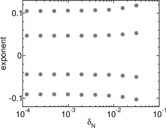
Figure 2: Effective exponents of $\frac{4}{(M-1)^{2}}-|t_{\nu,\nu^{\prime}}|^{2}$ (circles) and $|t_{\nu,M}|^{2}$ (stars) as a function of $\delta_{N}$ for $M=5$, $\tilde{t}=1$, $t_{M}=10^{-3}$, and different values of $U=-1,-0.5,0.5,1$ from top to bottom. On the scale of the plot the results obtained from $\frac{4}{(M-1)^{2}}-|t_{\nu,\nu^{\prime}}|^{2}$ and $|t_{\nu,M}|^{2}$ are indistinguishable. The scaling exponent is read-off when a plateau is reached for $\delta_{N}<5\cdot 10^{-4}$, which roughly corresponds to $N>10^{4}$.

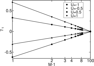
Figure 3: Scaling exponent of the conductance for a weak link as a function of $M-1$ (symbols) for different $U$. Note the reciprocal scale of the $x$-axis. The lines show $\gamma_{1}(M)=\beta_{s}/(M-1)$.

The $M$-dependence of the scaling exponent for different $U$ is shown in Fig. 3 on a reciprocal-linear scale (symbols). The data can be fitted by (lines)

$$\gamma_{1}(M)=\beta_{s}/(M-1)\,,$$ (53)

with $\beta_{s}$ being the $U$-dependent fRG approximation for $2\alpha_{B}=2(1/K-1)$ obtained in Ref. Enss04, for a weak link (strong impurity) in an infinite wire, i.e. the $M=2$ case. The exponent $\beta_{s}$ agrees with $2\alpha_{B}$ to leading order in $U$. It has higher order corrections which bring it close to $2\alpha_{B}$ even for intermediate $U$. For the four interactions $U=-1,-0.5,0.5,1$ the value for $\beta_{s}$ can be read off from Fig. 3. At $U=1$ the relative difference between the exact exponent obtained from Eq. (6) and our approximation is roughly 5%. A detailed comparison of $\beta_{s}$ and $2\alpha_{B}$ is given in Fig. 5 of Ref. Enss04, . To leading order in $U$ Eq. (53) confirms the result deduced from the combined use of the HFA and Fermi’s golden rule arguments Eq. (52). For $M=2$, the fRG approximation $\beta_{s}$ is generically closer to the exact exponent $2\alpha_{B}$ than $2\alpha_{B}^{\rm HF}$.

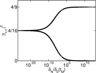
Figure 4: One-parameter scaling plot of the effective transmissions $|t_{\nu,M}|^{2}$ (lower curve) and $|t_{\nu,\nu^{\prime}}|^{2}$ with $\nu,\nu^{\prime}\leq M-1$ (upper curve) for $M=4$, $U=-1$, and $\tilde{t}=1$. The variable is $\delta_{N}/\delta_{0}(t_{M})$, with a non-universal scale $\delta_{0}(t_{M})$. The asymptotic values of the transmission $4/(M-1)^{2}$ and $0$ reached for $\delta_{N}/\delta_{0}(t_{M})\to\infty$ as well as $4/M^{2}$ reached for $\delta_{N}/\delta_{0}(t_{M})\to 0$ are indicated on the $y$-axis.

For $U>0$, $\gamma_{1}>0$ and the “perfect junction” FP of the $(M-1)$-wire system is stable towards weakly coupling an additional wire, while for $U<0$, $\gamma_{1}<0$ and the FP is unstable. In the latter case the system effectively incorporates the weakly coupled leg and flows to the “perfect junction” FP for $M$ wires. For small to intermediate $|U|$ and starting close to the “perfect junction” FP of the $(M-1)$-wire system, i.e. for $t_{M}\ll\tilde{t}$, exponentially small $\delta_{N}$ are required to reach the new FP. Even though we can treat very large $N$ such small scales are beyond the possibilities of our method. Similar to the single impurity problemKaneFisher ; Fendley ; VM4 ; Enss04 the flow from one to the other FP can be shown considering data sets $(\delta_{N},|t_{\nu,\nu^{\prime}}|^{2})$ obtained for different $t_{M}\in]0,1[$ using a one-parameter scaling ansatz. For fixed $U$ the conductance is only a function of $\delta_{N}/\delta_{0}(t_{M})$, with an appropriately chosen non-universal energy scale $\delta_{0}(t_{M})$ and the different data sets can be collapsed on a single curve. This is shown in Fig. 4 for the two different effective transmissions $|t_{\nu,M}|^{2}$ (lower curve) and $|t_{\nu,\nu^{\prime}}|^{2}$ with $\nu,\nu^{\prime}\leq M-1$ (upper curve) and $M=4$, $U=-1$, $\tilde{t}=1$ on a log-linear scale. It is important to note that the effective transmission $4/M^{2}$ between all legs is not achieved by an increase of $t_{M}$. As there is no interaction across the links of the dot to the first sites of the wires, the hopping across these links is independent of the RG cutoff (here $\delta_{N}$). The transmission $4/M^{2}$ follows from the build up of a self-energy during the RG flow, that, interpreted as an effective scattering potential, leads to a resonance at the chemical potential. For $\gamma_{1}<0$, that is $U<0$, the plateau reached in Fig. 2 does not present the asymptotic behavior for $\delta_{N}\to 0$ and considering even smaller $\delta_{N}$ a deviation from the plateau value $\gamma_{1}$ can be observed.

We next show that the scaling behavior of the conductance can be understood from the scaling of the spectral weights on the first site of one of the equivalent legs and the first site of the additional wire. For $\varepsilon=0$ we get from Eq. (25)

$$|t_{\nu,\nu^{\prime}}|^{2}=\frac{4}{(M-1)^{2}}-\frac{8}{(M-1)^{3}}D+{\mathcal{O}}(\tau^{4})\;,$$ (54)

for $\nu\neq\nu^{\prime}$ and $\nu,\nu^{\prime}\leq M-1$, as well as

$$|t_{\nu,M}|^{2}=\frac{4}{(M-1)^{2}}D-\frac{8}{(M-1)^{3}}D^{2}+{\mathcal{O}}(\tau^{6})\,,$$ (55)

for $\nu\leq M-1$, with

$$D=\Delta_{M}(0)/\Delta\propto\tau^{2}\;.$$ (56)

For the reflection back into wire $\nu\leq M-1$ it follows

$$R_{\nu} =1-\sum_{\nu^{\prime}\neq\nu}|t_{\nu,\nu^{\prime}}|^{2}$$

$$=\frac{(M-3)^{2}}{(M-1)^{2}}+\frac{4}{(M-1)^{2}}\left[1-\frac{2}{(M-1)}\right]D$$

$$+\frac{8}{(M-1)^{3}}D^{2}+{\mathcal{O}}(\tau^{6})\;.$$ (57)

As discussed in Sect. III the auxiliary Green function is calculated with a self-energy which has been determined in the presence of the weak link. Thus $\Delta/\tilde{t}^{2}$ and the spectral weight $\rho_{1}$ of a perfect $(M-1)$-leg junction differ to order $\tau^{2}$. If corrections of order $\tau^{2}$ are neglected in $\Delta$ and $\Delta_{M}(0)$, $D$ can be replaced by $\rho_{\rm obc}/\rho_{1}$. We numerically find that for $\tilde{M}=1,2,\ldots$ the spectral weight on the first site of a perfect $\tilde{M}$-leg junction scales as

$$\rho_{1}\propto\delta_{N}^{-\alpha^{\rm fRG}_{\tilde{M}}}\;,$$ (58)

with

$$\alpha_{\tilde{M}}^{\rm fRG}=\frac{\beta_{s}}{2}\left(\frac{2}{\tilde{M}}-1\right)\;,$$ (59)

consistent with the derivation using the HFA in Eq. (49). The above replacement thus leads to $D\propto\delta_{N}^{\beta_{s}/(M-1)}$, where we used $\rho_{\rm obc}\propto\delta_{N}^{\beta_{s}/2}$. Inserting this expression in Eqs. (54) and (55) we reproduce the results directly obtained from calculating the effective transmission. Note that for $M=3$ the second term in Eq. (V.1.1) cancels and the reflection scales with an exponent that is twice as large as the one of the transmission. Further down we encounter another case in which the prefactor of the leading order term vanishes for specific parameters, which leads to a doubling of the scaling exponent.

In the limit $M\to\infty$ the dot site is coupled to so many legs that it creates an infinite barrier. Consistently Eq. (59) gives $\lim_{M\to\infty}\alpha_{M}^{\rm fRG}=-\frac{\beta_{s}}{2}$ and the spectral weight on the first sites scales as the weight next to an open boundary.

V.1.2 A slightly modified link

As the second example with a single modified link we consider $|t_{M}-\tilde{t}|/\tilde{t}=\tau\ll 1$. We now analyze the scaling of the effective transmission within the subsystem of the $M-1$ equivalent wires and into the leg with the modified hopping with respect to the transmission $4/M^{2}$ of the perfect case. Similarly to Fig. 2 exponents can reliably be extracted for sufficiently large $N$.

For $M\geq 3$ the exponents of $|t_{\nu,\nu^{\prime}}|^{2}$ and $|t_{\nu,M}|^{2}$, with $\nu,\nu^{\prime}\in[1,M-1]$ turn out to be equal. For several $U$ the $M$-dependence of the scaling exponent is shown in Fig. 5 on a reciprocal-linear scale. To first order in $U$ it is given by $-\beta_{s}/M$. More accurately the data can be fitted by

$$\gamma_{2}(M)=-\frac{\beta_{s}}{M}+2\frac{\beta_{w}+\beta_{s}}{M^{2}}\;,$$ (60)

with the exponent $\beta_{w}$ found in Ref. Enss04, for the scaling of the transmission through a local weak impurity. To leading order in $U$, $\beta_{w}$ agrees with the exact weak single impurity exponent $2(K-1)$. A comparison of $2(K-1)$ and our fRG approximation is given in Fig. 7 of Ref. Enss04, .

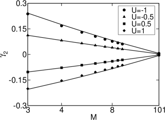
Figure 5: Scaling exponent of the conductance for a slightly modified link as a function of $M$ for different $U$. Note the reciprocal scale of the $x$-axis. The lines show the fit Eq. (60).

For $U>0$, $\gamma_{2}<0$ and the “perfect junction” FP of the $M$-wire system is unstable towards changing one of the hopping amplitudes. For $t_{M}<\tilde{t}$ the system flows to the “perfect junction” FP of $M-1$ wires. This follows from the build up of a self-energy during the RG flow, that leads to a vanishing transmission from wire $\nu\leq M-1$ to wire $M$, but to a resonance with perfect transmission between the $M-1$ equivalent legs. For $t_{M}>\tilde{t}$ the flow is to a FP with vanishing conductance between all wires – the “decoupled chain” FP. The vanishing of the conductance follows from the long-range oscillatory behavior of the self-energy generated in the RG flow. In both cases the flow from one to the other FP can again be shown using a one-parameter scaling ansatz. For $U<0$, $\gamma_{2}>0$ and the “perfect junction” FP of the $M$-wire system is stable, regardless of the sign of $\tilde{t}-t_{M}$.

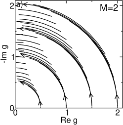
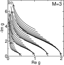
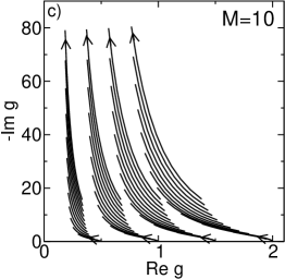
Figure 6: Flow of $g$ Eq. (63) for the case of a symmetric junction with on-site energy $V=0.5,1,1.5,2$, different $\tilde{t}\in[0.01,0.7]$, $M=2,3,10$ legs, and $U=-1$. The arrows indicate the direction of the flow for $U<0$. For $U>0$ it is reversed.

For $M=2$ there is no $|t_{\nu,\nu^{\prime}}|^{2}$ and $1-|t_{\nu,M}|^{2}$ scales with $2\gamma_{2}(2)$. The appearance of the factor $2$ can be explained by considering an expansion of $|t_{\nu,M}|^{2}$ similar to Eqs. (54) and (55) (which is valid for all $M\geq 2$)

$$|t_{\nu,M}|^{2} = \frac{4}{M^{2}}+\frac{4(D-1)}{M^{2}}\left(1-\frac{2}{M}\right)$$ (61)

$$-\frac{4(D-1)^{2}}{M^{3}}\left(2-\frac{3}{M}\right)\;,$$

with $D$ as defined in Eq. (56). The difference $D-1$ shows power-law scaling with exponent $\gamma_{2}(M)$. For $M=2$ the prefactor of the leading order term linear in $D-1$ vanishes and the scaling exponent of $|t_{\nu,M}|^{2}$ is doubled. Inserting $M=2$ in Eq. (60) gives $2\gamma_{2}(2)=\beta_{w}$ as the exponent characterizing the deviation from transmission $1$. This result is expected since the case $M=2$ corresponds to the situation of a perfect infinite wire interrupted by a small impurity characterized by the scaling exponent $\beta_{w}\approx 2(K-1)$.

In the single impurity problem the fRG approximations $\beta_{s}$ for $2\alpha_{B}=2(1/K-1)$ and $\beta_{w}$ for $2(K-1)$ are correct to order $U$. To leading order $2(K-1)\approx-2(1/K-1)$ [see Eq. (6)] and the second term in Eq. (60) is of order $U^{2}$. As terms of order $U^{2}$ are only partly included in our approximation scheme it is questionable if a term similar to the second one will be present in the (unknown) exact expression for $\gamma_{2}$. To derive the dependence of $\gamma_{1}$ and $\gamma_{2}$ on $K$ and $M$ presents a challenge for any method which does not require approximations in the strength of the interaction.

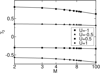
Figure 7: Scaling exponent of the conductance for a small on-site energy as a function of $M$ (symbols) for different $U$. Note the reciprocal scale of the $x$-axis. The lines show the fit Eq. (64).

V.2 A symmetric junction with a dot site energy

As our second specific case we study a symmetric $M$-leg junction with $t_{\nu}=\tilde{t}$ for $\nu=1,\ldots,M$ and a non-vanishing dot site energy $V$. Then, due to symmetry, all $\Omega_{\nu}(0)$ and $\Delta_{\nu}(0)$ [see Eq. (26)] are equal and we suppress the index $\nu$. Eq. (25) simplifies to

$$|t|^{2}=\frac{4}{M^{2}}\;\frac{M^{2}\Delta^{2}(0)}{\left[V+M\Omega(0)\right]^{2}+M^{2}\Delta^{2}(0)}\;.$$ (62)

The transmission is determined by the single complex parameter

$$g=V+M\Omega(0)-iM\Delta(0)=-\,\frac{1}{{\mathcal{G}}_{d}(0+i0)}\;,$$ (63)

which itself is a function of the junction parameters $(\tilde{t},V)$ and $M$. Via the RG flow of the self-energy for $U\neq 0$ it moreover develops a dependence on $\delta_{N}$ and the interaction $U$. The RG flow can nicely be visualized by plotting $g$ in the complex plane with $\delta_{N}$ as a parameter.Enss04 ; Xavier This is done in Figs. 6a) to 6c) for $M=2,3,10$, $V=0.5,1,1.5,2$, and different $\tilde{t}\in[0.01,0.7]$. For decreasing $\delta_{N}\in[5\cdot 10^{-4},2.5\cdot 10^{-1}]$ and $U\neq 0$ each fixed parameter set $(\tilde{t},V)$ leads to a flow line. The general form of the flow diagrams is independent of the absolute value of $U$. The data of the figures were calculated for $U=-1$, which leads to the flow direction indicated by the arrows. For $U>0$ the direction is reversed. On the line $\mbox{Im}\,g=0$ the conductance vanishes and the $x$-axis forms a line of “decoupled chain” FPs. For $\mbox{Re}\,g=0$ the transmission is $4/M^{2}$ and all points on the $y$-axis are “perfect junction” FPs (line of FPs). The “perfect junction” transmission $4/M^{2}$ is also reached at $g=\infty$ provided that this point is approached such that $-\mbox{Im}\,g\to\infty$ and $\mbox{Re}\,g$ goes to a constant.

For $M=2$ the flow approximately follows a section of a circle centered around the origin with a radius $V$. For $U<0$ the direction is counter-clockwise and the line of “perfect junction” FPs ($y$-axis) is stable. The on-site energy $V$ does not get renormalized in the RG flow as the interaction between the dot site and the first sites of the wires is assumed to be $0$. The perfect transmission $4/M^{2}$ does thus not follow from a decrease of $V$ during the RG flow but is a consequence of the spatial structure of the self-energy, which leads to a a resonance at the chemical potential. For $U>0$ the flow is clockwise and the line of “perfect junction” FPs is unstable. The system flows to the line of stable “decoupled chain” FPs. The vanishing of the conductance is a consequence of the long-range oscillatory dependence of the self-energy on $j$. For $M\geq 3$, $U<0$, and $\delta_{N}\to 0$, -$\mbox{Im}\,g$ diverges while $\mbox{Re}\,g$ goes to a constant, which implies that the system reaches a “perfect junction” FP. For $U>0$ all trajectories approach the $x$-axis at $V$ and the conductance vanishes (line of “decoupled chain” FPs). To determine scaling exponents we next separately consider small and large $V$.

V.2.1 A small on-site energy

For small $V$, the transmission between all the equivalent wires is close to the perfect value $4/M^{2}$. The dependence on $\delta_{N}$ can be described by a power-law. In Fig. 7 the scaling exponent as a function of $M$ is shown for different $U$. To leading order in $U$ it is independent of $M$. The exponent can be fitted by

$$\gamma_{3}(M)=-\beta_{s}+4\frac{\beta_{w}+\beta_{s}}{M}\left(1-\frac{1}{M}\right)\;.$$ (64)

In accordance with the stability properties of the line of “perfect junction” FPs discussed in connection with Figs. 6a) to 6c), $\gamma_{3}<0$ for $U>0$ and $\gamma_{3}>0$ for $U<0$. The $M=2$ case is equivalent to the problem of a single weak site impurity interrupting an otherwise perfect infinite chain and $\gamma_{3}(2)$ is equal to the respective scaling exponent $\beta_{w}$ (similar as for a slightly modified link in Sect. V.1). Within our approximation scheme the second term in Eq. (64) is thus important to reproduce a result obtained earlier for $M=2$. As it is of order $U^{2}$ it is nonetheless unclear if a similar term occurs in the (unknown) exact expression for $\gamma_{3}$.

V.2.2 A large on-site energy

In the limit of large $V$ the transmission between all the wires is small and we analyze the scaling with respect to zero transmission. The scaling exponent is independent of $M$ and up to our numerical accuracy given by

$$\gamma_{4}=\beta_{s}\;,$$ (65)

i.e. the strong impurity (weak link) exponent for a single infinite wire (see Fig. 5 of Ref. Enss04, ).

V.3 Fixed points and renormalization group flow for general junction parameters

The RG flow, FP structure, and scaling exponents for arbitrary junction parameters can be understood based on the results obtained for the above two classes of junction parameters. To shorten the discussion we here focus on the more important case $U>0$. Results for $U<0$ can be deduced by inverting the direction of the flow.

As found in subsections V.1 and V.2 the “perfect junction” FP of the $M$-leg system with effective transmission $4/M^{2}$ is unstable towards the two possible perturbations in which only one junction parameter is modified: (i) a single modified hopping and (ii) a non-vanishing on-site energy. These instabilities are characterized by the two exponents $\gamma_{2}(M)$ (modified link) and $\gamma_{3}(M)$ (on-site energy).

In the case (i), for $M\geq 3$, and $\tilde{t}$ larger than the single modified hopping the system flows to the “perfect junction” FP for $M-1$ legs. For $\delta_{N}\to 0$ the conductance across the modified link vanishes with exponent $\gamma_{1}(M)$, while the conductance within the subsystem of the $M-1$ equivalent wires approaches $4/(M-1)^{2}$ with the same exponent. For $M=2$ the flow is to the “decoupled chain” FP and the conductance vanishes with exponent $\gamma_{1}(2)=\gamma_{4}=\beta_{s}$. If the hopping between the first site of wire $\nu=M$ and the dot site is larger than $\tilde{t}$ for $\delta_{N}\to 0$ and all $M\geq 2$ the “decoupled chain” FP is reached. To analyze the scaling of the conductance close to this FP we start out from Eq. (25) and use an expansion similar to Eqs. (54) and (55). The small parameter of the expansion is $D=\Delta/\Delta_{M}$. The numerics shows that it asymptotically vanishes as $\delta_{N}^{\beta_{s}}$. For $\nu\leq M-1$ this leads to

$$G_{\nu,M}\propto\delta_{N}^{\gamma_{4}}$$ (66)

while for $\nu,\nu^{\prime}\in[1,M-1]$ we find

$$G_{\nu,\nu^{\prime}}\propto\delta_{N}^{2\gamma_{4}}\;.$$ (67)

In the case (ii) the RG flow also ends at the “decoupled chain” FP and all conductances vanish with exponent $\gamma_{4}$.

We next perturb the “perfect junction” FP of the $M$-leg system by slightly modifying more than one of the hopping matrix elements. If $2\leq M_{1}<M-1$ of the $t_{\nu}$ are reduced compared to the hopping $\tilde{t}$ across the remaining $M_{2}=M-M_{1}$ links the system flows to the “perfect junction” FP of the $M_{2}$-leg system. If $M_{1}$ of the $t_{\nu}$ are increased compared to $\tilde{t}$ the system generically approaches the “decoupled chain” FP. This behavior is changed if $\tilde{M}_{1}\geq 2$ of the $M_{1}$ increased hoppings are equal and larger than all the others. In this case the system flows to the “perfect junction” FP for $\tilde{M}_{1}$ legs. If all $t_{\nu}$ are different the “decoupled chain” FP is reached.

If the perturbation of the “perfect junction” FP of the $M$-leg system consists of an on-site energy $V$ and one or more modified hoppings the system flows to the “decoupled chain” FP.

From these considerations we conclude that for the majority of possible junction parameters of the $M$-wire junction, for $\delta_{N}\to 0$ the system flows to the “decoupled chain” FP. On asymptotically small scales the conductance vanishes as

$$G_{\nu,\nu^{\prime}}\propto\delta_{N}^{\xi\beta_{s}}\;.$$ (68)

Depending on the junction parameters as well as on the wire indices $\nu$ and $\nu^{\prime}$, $\xi$ might be $1$ or $2$ (for examples, see above).

Only for $V=0$ and if $M_{\rm max}\geq 2$ of the $M$ links between the dot site and the first lattice sites of the wires have hopping $t_{\rm max}$, where $t_{\rm max}=\max_{\nu\in[1,M]}\{t_{\nu}\}$, the system flows to the “perfect junction” FP for $M_{\rm max}$ legs. In this case the power-law scaling of the conductance between two wires coupled to the dot with hopping $t_{\rm max}$ is given by

$$\frac{e^{2}}{h}\,\frac{4}{M_{\rm max}^{2}}-G_{\nu,\nu^{\prime}}\propto\delta_{N}^{\beta_{s}/M_{\rm max}}\;.$$ (69)

The conductance between one wire coupled by $t_{\rm max}$ and the other by $t_{\nu}<t_{\rm max}$ vanishes as

$$G_{\nu,\nu^{\prime}}\propto\delta_{N}^{\beta_{s}/M_{\rm max}}\;,$$ (70)

while it goes like

$$G_{\nu,\nu^{\prime}}\propto\delta_{N}^{2\beta_{s}/M_{\rm max}}\;.$$ (71)

if both wires $\nu$ and $\nu^{\prime}$ have a hopping to the dot site smaller than $t_{\rm max}$. As in Eq. (67) the factor $2$ in Eq. (71) follows from an expansion similar to the one used in Eqs. (54) and (55).

VI Summary and Perspectives

In this paper we studied the conductance $G_{\nu,\nu^{\prime}}$ for a dot junction of $M$ semi-infinite quantum wires. The junction as well as the wires are described by a microscopic lattice model. In a finite section of $N$ sites the fermions in each wire are modeled to interact via a nearest-neighbor interaction which smoothly vanishes close to the lattice sites $j=N$ (smooth contact). Investigating the scaling of the conductance as a function of $\delta_{N}\propto 1/N$ led to a comprehensive picture of the FP structure, scaling exponents, and RG flow of the model studied. We mainly used an approximation scheme that is based on the fRG method and provides reliable results for week to intermediate interactions with $1/2\leq K\leq 3/2$. At half-filling this corresponds to bulk nearest-neighbor interactions $-1.5\leq U\leq 2$. Additional insights were obtained using the HFA.

Compared to the well studied single impurity problem for $M\geq 3$ the low-energy physics of the $M$-wire junction is much richer, allowing for a variety of FPs and scaling exponents. Furthermore for $M\geq 3$ one of them, the “perfect junction” FP, is characterized by two exponents: $\gamma_{2}(M)$ and $\gamma_{3}(M)$. They can individually be read off from the scaling of the conductance if the FP is perturbed in a specific way. In contrast to the single impurity problem, in which the FP reached is solely determined by the sign of the interaction, for junctions of three and more wires this in addition depends on the junction parameters. Depending on the wire indices between which the conductance is calculated the scaling exponents close to a FP might differ by factors of two. This can have two reasons: (i) In an expansion of the effective transmission in terms of a small parameter that carries the power-law scaling [see e.g. Eqs. (54) and (55)], depending on $\nu$ and $\nu^{\prime}$ the first or second order term might be the first non-vanishing one. (ii) For certain $M$ the prefactor of the leading order term might vanish.

Junctions and networks of TLLs were earlier studied.Nayak ; Safi ; Lal ; Chen ; Claudio ; Das ; Doucot The method and model used in Ref. Lal, come closest to ours. The authors apply a fermionic poor-man’s like RG originally developed for the single impurity problem to the three- and four-leg junction.MatveevGlazman They consider a microscopic dot junction model to motivate the investigation but then leave the framework of this model when studying the RG flow of an effective $S$-matrix. The results obtained in this paper for three legs are partly equivalent to ours. In Refs. Enss04, and VMresotun, a detailed account of the differences of the poor-mans RG and our method is given for the single impurity case and resonant tunneling in a TLL.

Using the fRG and HFA we obtained expressions for the scaling exponents which we expect to be correct (at least) to leading order in $U$. It is very desirable to derive the exact $K$- and $M$-dependence of these exponents. For increasing complexity of the junctions obtaining such expressions for simplified, effective, but still generic models requires very sophisticated methods, even if only specific parts of the parameter space are considered.Claudio

We considered a dot junction model in which the interaction between fermions on the dot site and the first lattice sites of the wires is set to zero. We also investigated the case in which this interaction does not vanish. The additional nearest-neighbor interaction across the $M$ bonds does not alter the results presented here.

An extension of our method to the case in which the strength of the bulk interaction depends on the wire index $\nu$ is straightforward and might lead to new insights. As exemplified in Ref. Xavier, the fRG can also be used to investigate other types of junctions (e.g. ring like geometries), with different FPs and new scaling exponents.

For the complex junction studied here the temperature $T$ and the infrared cutoff $\delta_{N}$ present equivalent scaling variables only on asymptotically small scales. The fRG method can be set up for finite $T$ and leads to reliable results also for intermediate to large temperatures.Enss04 ; VMresotun For two wires our model is equivalent to the one considered to study resonant tunneling through a quantum dot embedded in a TLL, with a one lattice site dot. In this case, for fixed $N$, and $\delta_{N}\leq T\leq B$ the conductance as a function of $T$ shows a very rich behavior. Depending on the dot parameters, temperature regimes in which $G(T)$ follows “universal” power-laws as well as non-universal regimes were identified.Enss04 ; VMresotun We thus expect to find similar rich behavior for $M\geq 3$. The conductance as a function of temperature is easily accessible in transport experiments. Investigating $G_{\nu,\nu^{\prime}}(T)$ might thus also become important for the interpretation of future transport experiments on junctions of quasi one-dimensional quantum wires. We will present results for $G_{\nu,\nu^{\prime}}(T)$ in an upcoming publication.

References

- (1) For a review on Tomonaga-Luttinger liquid behavior see K. Schönhammer, in Interacting Electrons in Low Dimensions, Editor: D. Baeriswyl, Kluwer Academic Publishers (2004); cond-mat/0305035.
- (2) A. Luther and I. Peschel, Phys. Rev. B 9, 2911 (1974).
- (3) D. Mattis, J. Math. Phys. 15, 609 (1974).
- (4) C.L. Kane and M.P.A. Fisher, Phys. Rev. Lett. 68, 1220 (1992); Phys. Rev. B 46, 15233 (1992).
- (5) I. Safi and H.J. Schulz, Phys. Rev. B 52, R17040 (1995); D.L. Maslov and M. Stone, ibid.52, R5539 (1995); V.V. Ponomarenko, ibid.52, R8666 (1995).
- (6) M. Fabrizio and A. Gogolin, Phys. Rev. B 51, 17827 (1995).
- (7) A. Furusaki and N. Nagaosa, Phys. Rev. B 47, 4631 (1993).
- (8) K. Moon, H. Yi, C.L. Kane, S.M. Girvin, and M.P.A. Fisher, Phys. Rev. Lett. 71, 4381 (1993).
- (9) D. Yue, L.I. Glazman, and K.A. Matveev, Phys. Rev. B 49, 1966 (1994).
- (10) P. Fendley, A.W.W. Ludwig, and H. Saleur, Phys. Rev. Lett. 74, 3005 (1995).
- (11) V. Meden, S. Andergassen, W. Metzner, U. Schollwöck, and K. Schönhammer, Europhys. Lett. 64, 769 (2003).
- (12) T. Enss, V. Meden, S. Andergassen, X. Barnabé-Thériault, W. Metzner, and K. Schönhammer, accepted for publication in Phys. Rev. B, cond-mat/0411310.
- (13) M.S. Fuhrer, J. Nygård, L. Shih, M. Forero, Y.-G. Yoon, M. Mazzoni, H. Coi, J. Ihm, S. Louie, A. Zettl, and P. McEuen, Science 288, 494 (2000).
- (14) M. Terrones, F. Banhart, N. Grobert, J.-C. Charlier, H. Terrones, and P.M. Ajayan, Phys. Rev. Lett. 89, 075505 (2002).
- (15) C. Nayak, M.P.A. Fisher, A.W.W. Ludwig, and H.H. Lin, Phys. Rev. B 59, 15694 (1999)
- (16) I. Safi, P. Devillard, and T. Martin, Phys. Rev. Lett. 86, 4628 (2001).
- (17) S. Lal, S. Rao, and D. Sen, Phys. Rev. B 66, 165327 (2002).
- (18) S. Chen, B. Trauzettel, and R. Egger, Phys. Rev. Lett. 89, 226404 (2002).
- (19) C. Chamon, M. Oshikawa, and I. Affleck, Phys. Rev. Lett. 91, 206403 (2003).
- (20) S. Das, S. Rao, and D. Sen, Phys. Rev. B 70, 085318 (2004).
- (21) K. Kazymyrenko and B. Douçot, cond-mat/0407268 (unpublished).
- (22) X. Barnabé-Thériault, A. Sedeki, V. Meden, and K. Schönhammer, accepted for publication in Phys. Rev. Lett., cond-mat/0411612.
- (23) C. Wetterich, Phys. Lett. B 301, 90 (1993).
- (24) T. R. Morris, Int. J. Mod. Phys. A 9, 2411 (1994).
- (25) M. Salmhofer, Renormalization, (Springer, Berlin, 1998).
- (26) V. Meden, T. Enss, S. Andergassen, W. Metzner, and K. Schönhammer, Phys. Rev. B 71, 041302(R) (2005).
- (27) V. Meden, W. Metzner, U. Schollwöck, O. Schneider, T. Stauber, and K. Schönhammer, Eur. Phys. J. B 16, 631 (2000).
- (28) V. Meden and U. Schollwöck, Phys. Rev. B 67, 193303 (2003).
- (29) F.D.M. Haldane, Phys. Rev. Lett. 45, 1358 (1980).
- (30) A. Oguri, J. Phys. Soc. Japan 70, 2666 (2001).
- (31) S. Andergassen, T. Enss, V. Meden, W. Metzner, U. Schollwöck, and K. Schönhammer, Phys. Rev. B 70, 075102 (2004).
- (32) V. Meden, W. Metzner, U. Schollwöck, and K. Schönhammer, Phys. Rev. B 65, 045318 (2002).