Vlasov analysis of relaxation and meta-equilibrium

Abstract

The Hamiltonian Mean-Field model (HMF), an inertial $XY$ ferromagnet with infinite-range interactions, has been extensively studied in the last few years, especially due to its long-lived meta-equilibrium states, which exhibit a series of anomalies, such as, breakdown of ergodicity, anomalous diffusion, aging, and non-Maxwell velocity distributions. The most widely investigated meta-equilibrium states of the HMF arise from special (fully magnetized) initial conditions that evolve to a spatially homogeneous state with well defined macroscopic characteristics and whose lifetime increases with the system size, eventually reaching equilibrium. These meta-equilibrium states have been observed for specific energies close below the critical value 0.75, corresponding to a ferromagnetic phase transition, and disappear below a certain energy close to 0.68. In the thermodynamic limit, the $\mu$-space dynamics is governed by a Vlasov equation. For finite systems this is an approximation to the exact dynamics. However, it provides an explanation, for instance, for the violent initial relaxation and for the disappearance of the homogeneous states at energies below 0.68.

I Introduction

Consider the one-dimensional Hamiltonian

$$H=\frac{1}{2}\sum_{i=1}^{N}p_{i}^{2}+\frac{J}{2N}\sum_{i,j=1}^{N}\left[1-\cos(\theta_{i}-\theta_{j})\right]\;.$$ (1)

It represents a lattice of classical spins with infinite-range interactions. Each spin rotates in a plane and is therefore described by an angle $-\pi\leq\theta_{i}<\pi$, and its conjugate angular momentum $p_{i}$, with $i=1,\ldots,N$; the constant $J$ is the interaction strength. Of course, one can also think of point particles of unitary mass moving on a circle. This model is known in the literature as mean-field XY-Hamiltonian (HMF)antoni95 .

The HMF has been extensively studied in the last few years (see reviewHMF for a review). The reasons for such interest are various. From a general point of view, the HMF can be considered the simplest prototype for complex, long-range systems like galaxies and plasmas (in fact, the HMF is a descendant of the mass-sheet gravitational modelantoni95 ). But the HMF is also interesting for its anomalies, be them model-specific or not. Especially worth of mention are the long-lived meta-equilibrium states (MESs) observed in the ferromagnetic HMF. These states exhibit breakdown of ergodicity, anomalous diffusion, and non-Maxwell velocity distributions, among other anomaliesmetastable ; plr (see also the contribution by A. Rapisarda et al. in this volume). It has been conjectured that it may be possible to give a thermodynamic description of these MESs by extending the standard statistical mechanics along the lines proposed by Tsallistsallis .

The simplicity of the HMF makes possible a full analysis of its equilibrium statistical properties, either in the canonicalantoni95 or microcanonical ensemblesantoni02 . If interactions are attractive ($J>0$), the system exhibits a ferromagnetic transition at the critical energy $E_{c}=0.75JN$. Here we will focus on the out-of-equilibrium behavior of the ferromagnetic HMF ($J>0$), when the system is prepared in a fully magnetized configuration, at an energy close below $E_{c}$, with uniformly distributed momenta (“water-bag” initial conditions). Under these initial conditions the system evolves to a spatially homogeneous state with well defined macroscopic characteristics and whose lifetime increases with the system size, eventually reaching equilibrium. Numerical experiments have shown the disappearance of the family of homogeneous MESs below a certain energy close to $0.68JN$.

II Equations of motion

It is convenient to write the Hamiltonian (1) in the simplified form:

$$H=\frac{1}{2}\sum_{i=1}^{N}p_{i}^{2}+\frac{N}{2}\left(1-m^{2}\right),$$

where we have introduced the magnetization per particle

$${\bf m}=\frac{1}{N}\sum_{i=1}^{N}\hat{\bf r}_{i}\;,\;\;\;\;\;\mbox{with}\;\;\;\hat{\bf r}_{i}=(\sin\theta_{i},\cos\theta_{i})\;,$$

and for simplicity we have taken $J=1$. The equations of motion read

$$\dot{\theta}_{i}\;=\;\frac{\partial H}{\partial p_{i}}\,=\,p_{i},\;\;\;\;\;\;\;\dot{p}_{i}\;=\;-\frac{\partial H}{\partial\theta_{i}}\,=\,{\bf m}\cdot\hat{\bf\theta}_{i},$$

for $i=1,\ldots,N$, with $\hat{\bf\theta}_{i}=(\cos\theta_{i},-\sin\theta_{i})$. Without loss of generality, we can set the axes such that $m_{x}(t=0)=0$. If, additionally, the distribution of momenta is symmetrical, then $m_{x}(t)=0,\;\;\forall t$. In that case, the equations of motion become

$$\dot{\theta}_{i}\;=\;\frac{\partial H}{\partial p_{i}}\,=\,p_{i},\;\;\;\;\;\;\;\dot{p}_{i}\;=\;-\frac{\partial H}{\partial\theta_{i}}\,=\,-m(t)\sin\theta_{i}.$$

Notice that these equations can be seen as the equations for a pendulum with a time-dependent length.

III First stage of relaxation

Fully magnetized states violently relax to a state of vanishing magnetization, within finite size corrections. The most elementary approach to describing the relaxation of ${\bf m}$, from a given initial condition, is to perform a series expansion around $t=0$, i.e.,

$${\bf m}(t)=\sum_{k\geq 0}\frac{1}{k!}{c_{k}}\,t^{k}.$$

In our case, the initial condition is such that $m=1$ (with $m_{x}=0$), then one obtains the following coefficients for $m_{y}(t)$

$$c_{0} = 1$$

$$c_{2} = -\langle p^{2}\rangle_{0}$$

$$c_{4} = \langle p^{4}\rangle_{0}+4\langle p^{2}\rangle_{0}$$

$$c_{6} = -\Bigl{(}\langle p^{6}\rangle_{0}+26\langle p^{4}\rangle_{0}+16\langle p^{2}\rangle_{0}+18\langle p^{2}\rangle^{2}_{0}\Bigr{)}$$

$$\vdots$$

and $c_{\rm odd}=0$, where averages are calculated with the initial distribution of momenta $h(p)$. If $h(p)$ at $t=0$ is symmetrical around $p=0$, then $m(t)$ is an even function of $t$. In particular, if the initial condition is water-bag, i.e., $\theta_{i}=0,\forall i$ and additionally $p_{i}$ are uniformly distributed in the interval $[-p_{o},p_{o}]$, then (from Hamiltonian (1), $p_{o}=\sqrt{6\varepsilon}$, with $\varepsilon$ the energy per particle), one obtains

$$m_{y}(t)\;=\;1-\varepsilon t^{2}+\biggl{(}\frac{3\varepsilon^{2}}{10}+\frac{\varepsilon}{3}\biggr{)}t^{4}+\ldots\;.$$ (2)

The convergence of this series is very slow and, given that a general expression is not available, only the very short time of the relaxation can be described.

IV Vlasov equation

On the other hand, the evolution equation of the reduced probability density function (PDF) in $\mu$-space is formally equivalent to the Vlasov-Poisson systemantoni95

$$\frac{\partial f}{\partial t}\,+\,p\frac{\partial f}{\partial\theta}\,-\,\frac{\partial V}{\partial\theta}\frac{\partial f}{\partial p}\,=\,0,$$ (3)

where $V=-{\bf m}\cdot\hat{\bf r}(\theta)$ and ${\bf m}=\int d\theta\,\hat{\bf r}(\theta)\int dp\,f(\theta,p,t)$. If ${\bf m}=m\hat{y}$, then

$$\frac{\partial f}{\partial t}\,+\,p\frac{\partial f}{\partial\theta}\,-\,m\sin\theta\frac{\partial f}{\partial p}\,=\,0,$$ (4)

with

$$m(t)=\int_{-\pi}^{\pi}d\theta\,\cos\theta\int_{-\infty}^{\infty}dp\,f(\theta,p,t).$$ (5)

The Vlasov equation (4) can be cast in the form

$$\frac{\partial f}{\partial t}\;=\;\left[{L}_{0}+{L}_{1}(t)\right]f,$$

where ${L}_{0}=-p\partial_{\theta}$ and ${L}_{1}(t)=m(t)\sin\theta\partial_{p}$. We will consider states (for instance, with vanishing magnetization) for which the term $L_{1}(t)$ can be treated as a perturbation. It is convenient to switch to the interaction representation, i.e., to define $\widetilde{f}(t)\;=\;{\rm e}^{-{L}_{0}t}f(t)$, then

$$\frac{\partial\widetilde{f}}{\partial t}\;=\;\widetilde{L}_{1}(t)\widetilde{f},$$

where $\widetilde{L}_{1}={\rm e}^{-{L}_{0}t}{L}_{1}{\rm e}^{{L}_{0}t}$.

The equation for the propagator $\widetilde{U}$, such that $\widetilde{f}(t)=\widetilde{U}(t)\widetilde{f}(0)$, is $\partial\widetilde{U}/\partial t=\widetilde{L}_{1}\widetilde{U}$, therefore,

$$\widetilde{U}(t)\;=\;1\;+\;\int_{0}^{t}dt^{\prime}\widetilde{L}_{1}(t^{\prime})\widetilde{U}(t^{\prime}),$$

and recursively, one has

$$\widetilde{U}(t)\;=\;1+\int_{0}^{t}dt_{1}\widetilde{L}_{1}(t_{1})+\int_{0}^{t}dt_{1}\widetilde{L}_{1}(t_{1})\int_{0}^{t_{1}}dt_{2}\widetilde{L}_{1}(t_{2})+\ldots\;.$$ (6)

The solution at order $k$ of the Vlasov Eq. (4) is

$$f^{(k)}(\theta,p,t)\;=\;{\rm e}^{-pt\partial_{\theta}}\widetilde{U}^{(k)}(t)f(\theta,p,0),$$ (7)

where the index $(k)$ indicates the order at which the expansion (6) is truncated. From here on, we will deal with continuous distributions, hence our treatment is valid in the thermodynamic limit.

IV.1 Lowest-order truncation

At zeroth-order, the propagator is approximated by $\widetilde{U}\simeq\widetilde{U}^{(0)}=1$. This is equivalent to neglecting the magnetization. Thus, if ${\bf m}=0$, the truncation is exact.

For the initial distribution $f(\theta,p,0)=g(\theta)h(p)$, where $g(\theta)$ is uniform in $[-\pi,\pi]$ (hence, ${\bf m}=0$) and $h(p)$ is an arbitrary even function, both distributions remain unaltered in time, consistently with the numerical simulations in Fig. 7 of plr . In fact, if ${\bf m}=0$ for any time, there are no forces to drive the system out of the macroscopic state.

If the initial condition is $f(\theta,p,0)=\delta(\theta)h(p)$, where $\delta$ is the Dirac delta function and $h(p)$ an arbitrary even function of $p$ (as in our case of interest), although $\bf m\neq 0$, $L_{1}$ is small (it is null at $t=0$ and remains small for later times), allowing a perturbative treatment. Then, we have

$$f^{(0)}(\theta,p,t)\;=\;{\rm e}^{-pt\partial_{\theta}}f(\theta,p,0)\;=\;h(p)\,\delta(\theta-pt)\;=\;\frac{1}{2\pi}h(p)\,\sum_{k=-\infty}^{\infty}{\rm e}^{ik(\theta-pt)}.$$

Therefore,

$$h^{(0)}(p,t)\;=\;\int_{-\pi}^{\pi}d\theta f^{(0)}(\theta,p,t)\;=\;h(p),$$

that is, at zeroth-order, the distribution of momenta, whatever it is, does not change in time. However the angular distribution does indeed change. For instance, in the particular case of the water-bag distribution, where $h(p)$ is a uniform distribution in $[-p_{o},p_{o}]$, we obtain

$$g^{(0)}(\theta,t)\;=\;\int_{-\infty}^{\infty}dpf^{(0)}(\theta,p,t)\;=\;\frac{1}{2\pi}\left(1+2\sum_{k\geq 1}\cos(k\theta)\frac{\sin(kp_{0}t)}{kp_{0}t}\right).$$ (8)

Notice that the distribution of angles becomes uniform in the long time limit. It gets uniform through a mechanism of phase mixing, where particles do not interact (remember that magnetization has been neglected). From Eqs. (5) and (8), the zeroth-order magnetization is

$$m^{(0)}(t)\;=\;\int_{-\pi}^{\pi}d\theta\cos\theta\,g^{(0)}(\theta,t)\;=\;\frac{\sin(p_{0}t)}{p_{0}t},$$ (9)

whose expansion in powers of time yields

$$m^{(0)}(t)\;=\;1-\varepsilon t^{2}+\frac{3}{10}\varepsilon^{2}t^{4}+\ldots$$

Observe that this expansion up to second-order coincides with the exact one, given by Eq. (2), for any $\varepsilon$.

IV.2 First-order truncation

Now, recalling that $\widetilde{U}^{(1)}=1+\int_{0}^{t}dt_{1}\widetilde{L}_{1}(t_{1})$, from (7), at first-order, we have

$$f^{(1)}(\theta,p,t) = {\rm e}^{-pt\partial_{\theta}}\widetilde{U}^{(1)}(t)f(\theta,p,0)$$

$$= f^{(0)}(\theta,p,t)+{\rm e}^{-pt\partial_{\theta}}\int_{0}^{t}dt_{1}\widetilde{L}_{1}(t_{1})f(\theta,p,0),$$

where $\widetilde{L}_{1}(t)={\rm e}^{pt\partial_{\theta}}\biggl{(}m(t)\sin\theta\,\partial_{p}\biggr{)}{\rm e}^{-pt\partial_{\theta}}$. Then

$$f^{(1)}(\theta,p,t)\;=\;h(p)\delta(\theta-pt) + h^{\prime}(p)\delta(\theta-pt)\int_{0}^{t}dt_{1}m(t_{1})\sin(\theta+pt_{1}-pt)$$

$$- h(p)\delta^{\prime}(\theta-pt)\int_{0}^{t}dt_{1}\,t_{1}m(t_{1})\sin(\theta+pt_{1}-pt)\;.$$

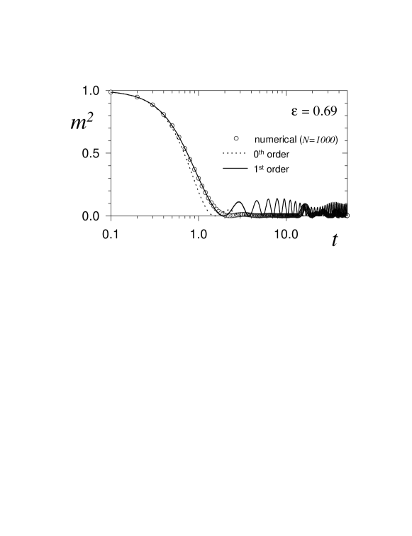
Figure 1: Squared magnetization as a function of time. The initial state is fully magnetized with uniformly distributed momenta for $\varepsilon=0.69$. Symbols correspond to numerical simulations with $N=1000$, the distribution of momenta is regular. Dashed lines correspond to the zeroth-order approximation obtained from Eq. (9). Full lines correspond to the first-order approximation given by Eq. (10)

After some algebra, for the case $h(p)$ uniform in $[-p_{o},p_{o}]$, we obtain

$$m^{(1)}(t)\;=\;m^{(0)}(t)\;+\;\int_{0}^{t}dt_{1}\,\frac{m(t_{1})}{2p_{0}}\biggl{(}\sin(p_{o}[t-t_{1}])+\frac{t_{1}-t}{t_{1}+t}\sin(p_{o}[t+t_{1}])\biggr{)}$$ (10)

Substituting $m(t)$ by $m^{(0)}(t)$ one obtains the magnetization at first-order. Moreover,

$$h^{(1)}(p,t)\;=\;\int_{-\pi}^{\pi}d\theta f^{(1)}(\theta,p,t)\;=\;h(p) + h^{\prime}(p)\int_{0}^{t}dt_{1}m(t_{1})\sin(pt_{1})$$

$$+ h(p)\int_{0}^{t}dt_{1}\,t_{1}m(t_{1})\cos(pt_{1})\;.$$

We recall that, for the uniform distribution, $h^{\prime}(p)\propto[\delta(p+p_{o})-\delta(p-p_{o})]$. This explains why $h(p,t)$ presents two spikes at $p=\pm p_{o}$.

Fig. 1 shows the first stage of the relaxation of the magnetization. Numerical simulations were performed for $N=1000$. Increasing the system size does not change the numerical curve in the time interval considered ($t\leq 50$). Of course, for longer times the curve becomes size dependentmetastable ; plr The squared magnetization rapidly decreases from its initial value $m^{2}=1$ down to zero at $t\simeq 2$. Then, it remains very close to zero up to $t\simeq 20$. From then on, one observes bursts of small amplitude. Since Vlasov equation is exact in the thermodynamic limit, it describes the exact $N=1000$ evolution up to time $t\simeq 50$. The zero order approximation describes correctly $m^{2}$ vs $t$ for a very short time ($t\simeq 0.4$). The first-order approximation describes satisfactorily the violent initial relaxation (up to $t\simeq 2$), but it does not reproduce the structure appearing later. Higher order corrections are required to describe that behavior. Extrapolation of numerical simulationsmetastable ; plr shows that $m\to 0$ in the thermodynamic limit. This regime settles for times beyond the scope of our approximation.

IV.3 Equilibrium

For completeness, let us discuss the distributions at thermal equilibriumvlasov_eq . If the system has already attained equilibrium, then $\partial_{t}=0$. Let also assume that the equilibrium distribution can be factorized, i.e., $f(\theta,p)\;=\;g(\theta)\,h(p)$. Then, from (4),

$$p\frac{\partial g}{\partial\theta}\,h(p)\;=\;m\sin\theta\,g(\theta)\frac{\partial h}{\partial p}.$$ (11)

Assuming $h(p)={A}\exp(-\beta p^{2}/[2\mu])$, Eq. (11) reduces to $\partial g/\partial\theta=-m\sin\theta\,g(\theta)$. Thus

$$g(\theta)\;=\;C{\rm e}^{\beta m\cos\theta},$$ (12)

with the normalization constant $C=1/[2\pi I_{0}(\beta m)]$, where $I_{0}$ is the modified Bessel function of zeroth-order. The equilibrium magnetization can be obtained from the consistency condition (5):

$$m\;=\;\int_{-\pi}^{\pi}d\theta\cos\theta\,g(\theta)\;=\;\frac{I_{1}(\beta m)}{I_{0}(\beta m)},$$

thus recovering the results of canonical calculationsantoni95 .

IV.4 Meta-equilibrium

Although we have not found the long-time solution of Vlasov equation, starting from fully magnetized initial conditions, numerical simulationsmetastable indicate that in the thermodynamic limit the system tends to a spatially homogeneous state. We have seen in Sect. IV.1 that, once reached a homogeneous state, the distribution of momenta, whatever it is, does not change in time. But, the question is whether the homogeneous solutions are stable or not under perturbations. On one hand, the Vlasov approach is a good approximation to the discrete dynamics, on the other finite-size effects may be the source of perturbations that may take the system out of a Vlasov steady state. Therefore, we will perform a stability test (valid in the thermodynamic limit) and discuss the results under the light of the discrete dynamics.

There is the well known Landau analysisbalescu which concerns linear stability. A more powerful stability criterion for homogeneous equilibria has been proposed by Yamaguchi et al.yamaguchi . This is a nonlinear criterion specific to the HMF. It states that $f(p)$ is stable if and only if the quantity

$$I\,=\,1\,+\,\frac{1}{2}\int_{-\infty}^{\infty}{\rm d}p\,\frac{f^{\prime}(p)}{p}$$ (13)

is positive (it is assumed that $f$ is an even function of $p$). This condition is equivalent to the zero frequency case of Landau’s recipeantoni95 ; choi03 . Yamaguchi et al.yamaguchi showed that a distribution which is spatially homogeneous and Gaussian in momentum becomes unstable below the transition energy $\varepsilon_{\rm cr}=3/4$ (see also choi03 ; inagaki93 ), in agreement with analytical and numerical results for finite $N$ systems. They also showed that homogeneous states with zero-mean uniform $f(p)$ are stable above $\varepsilon=7/12=0.58...$ (see also antoni95 ; choi03 ). In the same spirit, it is instructive to analyze the stability of the family of $q$-Gaussian distributions

$$f(p)\propto\exp_{q}(-\alpha p^{2})=\left[1-\alpha(1-q)p^{2}\right]^{1/(1-q)}\;,$$ (14)

which allows to scan a wide spectrum of PDFs, from finite-support to power-law tailed ones, containing as particular cases the Gaussian ($q=1$) and the water bag ($q=-\infty$). In Eq. (14), the normalization constant has been omitted and the parameter $\alpha>0$ is related to the second moment $\langle p^{2}\rangle$, which is finite only for $q<5/3$. In the homogeneous states of the HMF one has $\langle p^{2}\rangle=2\varepsilon-1$, as can be easily derived from Eq. (1). Then, the stability indicator $I$ as a function of the energy for the $q$-exponential family reads

$$I=1-\frac{3-q}{2(5-3q)(2\varepsilon-1)}\;.$$ (15)

Therefore, stability occurs for energies above $\varepsilon_{\rm q}$

$$\varepsilon_{\rm q}=\frac{3}{4}+\frac{q-1}{2(5-3q)}\;.$$ (16)

The stability diagram is exhibited in Fig. 2. It is easy to verify that one recovers the known stability thresholds for the uniform and Gaussian distributions. We remark that Eq. (16) states that only finite-support distributions, corresponding to $q<1$, are stable below $\varepsilon_{\rm cr}$. This agrees with numerical studies in the meta-equilibrium regimes of the HMF.

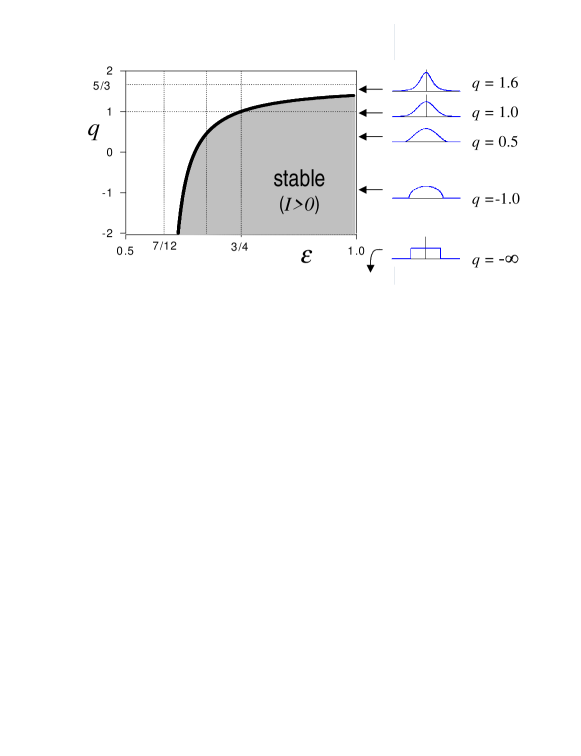
Figure 2: Stability diagram of the $q$-Gaussian ansatz for the momentum PDFs.

We have also shown recentlyvlasov that a similar analysis can be performed for a very simple family of functions exhibiting the basic structure of the observed $f(p)$, basically, a uniform distribution plus cosine. Fitting of numerical distributions leads to points in parameter space that fall close to the boundary of Vlasov stability, and exit the stability region for energies below the limiting value $\varepsilon\simeq 0.68$. This result is confirmed when the stability criterion is applied to the discrete distributions arising from numerical simulationsvlasov , although for the discrete dynamics the magnetization is not strictly zero.

The stability index $I$ is positive for energies above $\varepsilon\simeq 0.68$. The fact that the stability indicator becomes negative below $\varepsilon\simeq 0.68$ signals the disappearance of the homogeneous metastable phase at that energy. In fact, extrapolation of numerical simulations to the thermodynamic limit confirm this result. The present stability test only applies to homogeneous states. Strictly speaking, $m=0$ does not imply that the states are inhomogeneous. However, the sudden relaxation that leads to the present MESs mixes particlesplr in such a way that $m=0$ and spatial homogeneity are expected to be synonymous. Below $\varepsilon=0.68$, the measured distributions are evidently inhomogeneous ($m\neq 0$). In these cases, negative stability refers to hypothetical homogeneous states having the measured $f(p)$.

V Final remarks

We have seen that, although our approach is valid in the continuum limit, it gives useful hints on the finite size dynamics. Of course, it can not predict complex details of the discrete dynamics. However, the present approach gives information on the violent initial relaxation from fully magnetized states, for sufficiently large system. It also explains the disappearance of homogeneous MESs below a certain energy observed by extrapolation of numerical simulations to the thermodynamic limit. Moreover, the identification of MESs with Vlasov solutions is also consistent with the fact that when the thermodynamic limit is taken before the limit $t\to\infty$, the system never relaxes to true equilibrium, remaining forever in a disordered state.

References

- (1) M. Antoni and S. Ruffo, Phys. Rev. E 53, 2361 (1995).
- (2) T. Dauxois, V. Latora, A. Rapisarda, S. Ruffo and A. Torcini, in Dynamics and Thermodynamics of Systems with Long Range Interactions, edited by T. Dauxois, S. Ruffo, E. Arimondo and M. Wilkens, Lecture Notes in Physics Vol. 602, Springer (2002).
- (3) A. Torcini and M. Antoni, Phys. Rev. E 59, 2746 (1999). V. Latora, A. Rapisarda, and S. Ruffo, Physica A 280, 81 (2000); V. Latora, A. Rapisarda, and C. Tsallis, Phys. Rev. E 64, 056134 (2001); V. Latora and A. Rapisarda, Chaos, Solitons and Fractals 13, 401 (2002); A. Giansanti, D. Moroni, and A. Campa, ibid., p. 407; V. Latora, A. Rapisarda, and C. Tsallis, Physica A 305, 129 (2002); M. Montemurro, F. A. Tamarit and C. Anteneodo, Phys. Rev. E 67, 031106 (2003).
- (4) Pluchino, V. Latora and A. Rapisarda, Physica D 193, 315 (2003).
- (5) C. Tsallis, J. Stat. Phys. 52, 479 (1988); C. Tsallis, in Nonextensive Statistical Mechanics and its Applications, edited by S. Abe and Y. Okamoto, Lecture Notes in Physics Vol. 560 (Springer-Verlag, Heidelberg, 2001); Chaos, Solitons and Fractals 13, 371 (2002); Non Extensive Thermodynamics and Physical Applications, edited by G. Kaniadakis, M. Lissia, and A. Rapisarda, Physica A 305 (Elsevier, Amsterdam, 2002). See http://tsallis.cat.cbpf.br/biblio.htm for further bibliography on the subject.
- (6) M. Antoni, H. Hinrichsen, and S. Ruffo, Chaos, Solitons and Fractals 13, 393 (2002).
- (7) R. Balescu, Statistical Dynamics (Imperial College Press, London, 2000).
- (8) Y.Y. Yamaguchi, J. Barré, F. Bouchet, T. Dauxois and S. Ruffo, Physica A 337 , 36 (2004).
- (9) M.Y. Choi and J. Choi, Phys. Rev. Lett. 91, 124101 (2003).
- (10) S. Inagaki, Prog. Theo. Phys. 90, 577 (1993).
- (11) V. Latora, A. Rapisarda and S. Ruffo, Physica D 131, 38 (1999).
- (12) C. Anteneodo and R.O. Vallejos, Physica A 344, 383 (2004).