Focused Local Search for Random 3-Satisfiability

Abstract

A local search algorithm solving an NP-complete optimisation problem can be viewed as a stochastic process moving in an ’energy landscape’ towards eventually finding an optimal solution. For the random 3-satisfiability problem, the heuristic of focusing the local moves on the presently unsatisfied clauses is known to be very effective: the time to solution has been observed to grow only linearly in the number of variables, for a given clauses-to-variables ratio $\alpha$ sufficiently far below the critical satisfiability threshold $\alpha_{c}\approx 4.27$. We present numerical results on the behaviour of three focused local search algorithms for this problem, considering in particular the characteristics of a focused variant of the simple Metropolis dynamics. We estimate the optimal value for the “temperature” parameter $\eta$ for this algorithm, such that its linear-time regime extends as close to $\alpha_{c}$ as possible. Similar parameter optimisation is performed also for the well-known WalkSAT algorithm and for the less studied, but very well performing Focused Record-to-Record Travel method. We observe that with an appropriate choice of parameters, the linear time regime for each of these algorithms seems to extend well into ratios $\alpha>4.2$ — much further than has so far been generally assumed. We discuss the statistics of solution times for the algorithms, relate their performance to the process of “whitening”, and present some conjectures on the shape of their computational phase diagrams.

I Introduction

The 3-satisfiability (3-SAT) problem is one of the paradigmatic NP-complete problems GaJo79 . An instance of the problem is a formula consisting of $M$ clauses, each of which is a set of three literals, i.e. Boolean variables or their negations. The goal is to find a solution consisting of a satisfying truth assignment to the $N$ variables, such that each clause contains at least one literal evaluating to ’true’, provided such an assignment exists. In a random 3-SAT instance, the literals comprising each clause are chosen uniformly at random.

It was observed in MiSL92 that random 3-SAT instances change from being generically satisfiable to being generically unsatisfiable when the clauses-to-variables ratio $\alpha=M/N$ exceeds a critical threshold $\alpha_{c}$. Current numerical estimates BrMZ02 suggest that this satisfiability threshold is located approximately at $\alpha_{c}\approx 4.267$. For a general introduction to aspects of the satisfiability problem see DuGP97 .

Two questions are often asked in this context: how to solve random 3-SAT instances effectively close to the threshold $\alpha_{c}$, and what can be said of the point at which various types of algorithms begin to falter. Recently progress has been made by the “survey propagation” method BrMZ02 ; MeZe02 ; BrZ03 that essentially iterates a guess about the state of each variable, in the course of fixing an ever larger proportion of the variables to their “best guess” value.

In this article we investigate the performance of algorithms that try to find a solution by local moves, flipping the value of one variable at a time. When the variables to be flipped are chosen only from the unsatisfied (unsat) clauses, a local search algorithm is called focusing. A particularly well-known example of a focused local search algorithm for 3-SAT is WalkSAT SeKC96 , which makes “greedy” and random flips with a fixed probability. Many variants of this and other local search algorithms with different heuristics have been developed; for a general overview of the techniques see AaLe97 .

Our main emphasis will be on a focused variant of the standard Metropolis dynamics Metr53 of spin systems, which is also the base for the well-known simulated annealing optimization method. When applied to the 3-SAT problem, we call this dynamics the Focused Metropolis Search (FMS) algorithm. We also consider the Focused Record-to-Record Travel (FRRT) algorithm Duec93 ; SeOr03 , which imposes a history-dependent upper limit for the maximum energy allowed during its execution.

The space of solutions to 3-SAT instances slightly below $\alpha_{c}$ is known to develop structure. Physics-based methods from mean-field -like spin glasses imply through replica methods that the solutions become “clustered”, with a threshold of $\alpha\approx 3.92$ MeZe02 . The clustering implies that if measured e.g. by Hamming distance the different solutions in the same cluster are close to each other. A possible consequence of this is the existence of cluster “backbones”, which means that in a cluster a certain fraction of the variables is fixed, while the others can be varied subject to some constraints. The stability of the replica ansatz becomes crucial for higher $\alpha$, and it has been suggested that this might become important at $\alpha\approx 4.15$ MoPR04 . The energy landscape in which the local algorithms move is however a finite-temperature version. The question is how close to $\alpha_{c}$ one can get by moving around by local moves (spin flips) and focusing on the unsat clauses.

Our results concern the optimality of this strategy for various algorithms and $\alpha$. First, we demonstrate that WalkSAT works in the “critical” region up to $\alpha>4.2$ with the optimal noise parameter $p\approx 0.57$. Then, we concentrate on the numerical performance of the FMS method. In this case, the solution time is found to be linear in $N$ within a parameter window $\eta_{min}\leq\eta\leq\eta_{max}$, where $\eta$ is essentially the Metropolis temperature parameter. More precisely, we observe that within this window, the median and all other quantiles of the solution times normalised by $N$ seem to approach a constant value as $N$ increases. A stronger condition would be that the distributions of the solution times be concentrated in the sense that the ratio of the standard deviation and the average solution time decreases with increasing $N$. While numerical studies of the distributions do not indicate heavy tails that would contradict this condition, we can of course not at present prove that this is rigorously true. The existence of the $\eta$ window implies that for too large $\eta$ the algorithm becomes entropic, while for too small $\eta$ it is too greedy, leading to freezing of degrees of freedom (variables) in that case.

The optimal $\eta=\eta_{opt}(\alpha)$, i.e. that $\eta$ for which the solution time median is lowest, seems to increase with increasing $\alpha$. We have tried to extrapolate this behaviour towards $\alpha_{c}$ and consider it possible that the algorithm works, in the median sense, linearly in $N$ all the way up to $\alpha_{c}$. This is in contradiction with some earlier conjectures. All in all we postulate a phase diagram for the FMS algorithm based on two phase boundaries following from too little or too much greed. Of this picture, one particular phase space point has been considered before BaHW03 ; SeMo03 , since it happens to be the case that for $\eta=1$ the FMS coincides the so called Random Walk method Papa91 , which is known to suffer from metastability at $\alpha\approx 2.7$ BaHW03 ; SeMo03 .

The structure of this paper is as follows: In Section 2 we present as a comparison the WalkSAT algorithm, list some of the known results concerning the random 3-SAT problem, and test the WalkSAT for varying $p$ and $\alpha$ values. In Section 3 we go through the FMS algorithm in detail, and present extensive numerical simulations with it. Section 4 presents as a further comparison similar data for the FRRT algorithm. In Section 5 we discuss how the notion of whitening Pari02 is related to the behaviour of FMS with low $\eta$. Finally, section 6 finishes the paper with a summary.

II Local Search for Satisfiability

It is natural to view the satisfiability problem as a combinatorial optimisation task, where the goal for a given formula $F$ is to minimise the objective function $E=E_{F}(s)=$ the number of unsatisfied clauses in formula $F$ under truth assignment $s$. The use of local search heuristics in this context was promoted e.g. by Selman et al. in SeLM92 and by Gu in Gu92 . Viewed as a spin glass model, $E$ can be taken to be the energy of the system.

Selman et al. introduced in SeLM92 the simple greedy GSAT algorithm, whereby at each step the variable to be flipped is determined by which flip yields the largest decrease in $E$, or if no decrease is possible, then smallest increase. This method was improved in SeKC96 by augmenting the simple greedy steps with an adjustable fraction $p$ of pure random walk moves, leading to the algorithm NoisyGSAT.

WalkSAT(F,p):
  s = random initial truth assignment;
  while flips < max_flips do
    if s satisfies F then output s & halt, else:
    - pick a random unsatisfied clause C in F;
    - if some variables in C can be flipped without
      breaking any presently satisfied clauses,
      then pick one such variable x at random; else:
    - with probability p, pick a variable x
      in C at random;
    - with probability (1-p), pick some x in C
      that breaks a minimal number of presently
      satisfied clauses;
    - flip x.

Figure 1: The WalkSAT algorithm.

In a different line of work, Papadimitriou Papa91 introduced the very important idea of focusing the search to consider at each step only those variables that appear in the presently unsatisfied clauses. Applying this modification to the NoisyGSAT method leads to the WalkSAT SeKC96 algorithm (Figure 1), which is the currently most popular local search method for satisfiability.

In SeKC96 , Selman et al. presented some comparisons among their new NoisyGSAT and WalkSAT algorithms, together with some other methods. These experiments were based on a somewhat unsystematic set of benchmark formulas with $N\leq 2000$ at $\alpha\approx\alpha_{c}$, but nevertheless illustrated the significance of the focusing idea, since in the results reported, WalkSAT outperformed NoisyGSAT by several orders of magnitude.

More recently, Barthel et al. BaHW03 performed systematic numerical experiments with Papadimitriou’s original Random Walk method at $N=50,000$, $\alpha=2.0\dots 4.0$. They also gave an analytical explanation for a transition in the dynamics of this algorithm at $\alpha_{\mbox{\scriptsize dyn}}\approx 2.7$, already observed by Parkes Park02 . When $\alpha<\alpha_{\mbox{\scriptsize dyn}}$, satisfying assignments are generically found in time that is linear in the number of variables, whereas when $\alpha>\alpha_{\mbox{\scriptsize dyn}}$ exponential time is required. (Similar results were obtained by Semerjian and Monasson in SeMo03 , though with smaller experiments ($N=500$).) The reason for this dynamical threshold phenomenon seems to be that at $\alpha>\alpha_{\mbox{\scriptsize dyn}}$ the search equilibrates at a nonzero energy level, and can only escape to a ground state through a large enough random fluctuation. A rate-equation analysis of the method BaHW03 yields a very well matching approximation of $\alpha_{\mbox{\scriptsize dyn}}\approx 2.71$. See also SeMo04 for further analyses of the Random Walk method on random 3-SAT.

WalkSAT is more powerful than the simple Random Walk, because in it focusing is accompanied by other heuristics. However, it is known that the behaviour of WalkSAT is quite sensitive to the choice of the noise parameter $p$. E.g. Parkes Park01 experimented with the algorithm using a noise value $p=0.3$ and concluded that with this setting the algorithm works in linear time at least up to $\alpha=3.8$. Even this result is not the best possible, since it has been estimated Hoos02 ; HoSt99 ; WeSe02 that for random 3-SAT close to the satisfiability transition the optimal noise setting for WalkSAT is $p\approx 0.55$. (Actually our numerical experiments, reported below, suggest that the ideal value is closer to $p\approx 0.57$.)

These positive results notwithstanding, it has been generally conjectured (e.g. in BrMZ02 ) that no local search algorithm can work in linear time beyond the clustering transition at $\alpha_{d}\approx 3.92$. In a series of recent experiments, however, Aurell et al. AuGK04 concluded that with a proper choice of parameters, the median solution time of WalkSAT remains linear in $N$ up to at least $\alpha=4.15$, the onset of 1-RSB symmetry breaking. Our experiments, reported below, indicate that the median time in fact remains linear even beyond that, in line with our previous results SeOr03 .

(a) Complete data

(b) Medians and quartiles

Figure 2: Normalised solution times for WalkSAT, $\alpha=3.8\ldots 4.3$.

Figure 2 illustrates our experiments with the WalkSAT algorithm,  on randomly generated formulas of size $N=10^{5}$, various values of the noise parameter $p$, and values of $\alpha$ starting from $3.8$ and increasing at increments of $0.2$ up to $4.22$. For each $(p,\alpha)$-combination, 21 formulas were generated, and for each of these the algorithm was run until either a satisfying solution was found or a time limit of $80000\times N$ flips was exceeded. Figure 2(a) shows the solution times $t_{sol}$, measured in number of flips normalised by $N$, for each generated formula. Figure 2(b) gives the medians and quartiles of the data for each value of $\alpha$.

As can be seen from the figures, for value $p=0.45$ of the noise parameter WalkSAT finds satisfying assignments in roughly time linear in $N$, with the coefficient of linearity increasing gradually with increasing $\alpha$, up to approximately $\alpha=4.1$ beyond which the distribution of solution times for the algorithm diverges. For $p=0.55$, this linear regime extends further, up to at least $\alpha=4.18$, but for $p=0.65$ it seems to end already before $\alpha=3.9$. For the best value of $p$ we have been able to experimentally determine, $p=0.57$, the linear regime seems to extend up to even beyond $\alpha=4.2$.

(a) $\alpha=4.15$

(b) $\alpha=4.20$

Figure 3: Cumulative solution time distributions for WalkSAT with $p=0.55$.

To investigate the convergence of the solution time distributions, we tested the WalkSAT algorithm with $p=0.55$ at $\alpha=4.15$ and $\alpha=4.20$, in both cases with randomly generated sets of 100 formulas of sizes $N=10^{4},3\times 10^{4},10^{5},3\times 10^{5}$ and $10^{6}$. Figure 3 shows the cumulative distributions of the solution times normalised by $N$ achieved in these tests. As can be seen, for $\alpha=4.15$ the distributions are well-defined, with normalised medians and all other quantiles converging to a finite value for increasing $N$. However, for $\alpha=4.20$, the distributions seem to diverge, with median values increasing with increasing $N$.

Figure 4: Normalised solution times for WalkSAT with $\alpha=4.10\dots 4.22$, $p=0.50\dots 0.60$.

Figure 5: Cumulative solution time distributions for WalkSAT with $p=0.57$, $\alpha=4.20$.

In order to estimate the optimal value of the WalkSAT noise parameter, i.e. that value of $p$ for which the linear time regime extends to the biggest value of $\alpha$, we generated test sets consisting of 21 formulas, each of size $N=10^{5}$, for $\alpha$ values ranging from $4.10$ to $4.22$ at increments of $0.02$, and for each $\alpha$ for $p$ values ranging from $0.50$ to $0.60$ at increments of $0.01$. WalkSAT was then run on each resulting $(\alpha,p)$ test set; the medians and quartiles of the observed solution time distributions are shown in Figure 4. The data suggest that the optimal value of the noise parameter is approximately $p=0.57$. Figure 5 shows the empirical solution time distributions at $\alpha=4.20$ for $p=0.57$. In contrast to Figure 3(b), now the quantiles seem again to converge to a finite value for increasing $N$, albeit more slowly than in the case of the simpler $\alpha=4.15$ formulas presented in Figure 3(a).

III Focused Metropolis Search

From an analytical point of view, the WalkSAT algorithm is rather complicated, with its interleaved greedy and randomised moves. Thus, it is of interest to investigate the behaviour of the simpler algorithm obtained by imposing the focusing heuristic on a basic Metropolis dynamics Metr53 .

FMS(F,eta):
  s = random initial truth assignment;
  while flips < max_flips do
    if s satisfies F then output s & halt, else:
      pick a random unsatisfied clause C in F;
      pick a variable x in C at random;
      let x’ = flip(x), s’ = s[x’/x];
      if E(s’) <= E(s) then flip x, else:
         flip x with prob. eta^(E(s’)-E(s)).

Figure 6: The Focused Metropolis Search algorithm.

We call the resulting algorithm, outlined in Figure 6, the Focused Metropolis Search (FMS) method. The algorithm is parameterised by a number $\eta$, $0\leq\eta\leq 1$, which determines the probability of accepting a candidate variable flip that would lead to a unit increase in the objective function $E$. (Thus in customary Metropolis dynamics terms, $\eta=e^{1/T}$, where $T$ is the chosen computational temperature. Note, however, that detailed balance does not hold with focusing.)

(a) Complete data

(b) Medians and quartiles

Figure 7: Normalised solution times for FMS, $\alpha=3.8\ldots 4.3$.

We repeated the data collection procedure of Figure 2 for the FMS algorithm with various parameter values. The results for $\eta=0.2,0.3,0.4$ and $\eta=0.36$ (the best value we were able to find) are shown in Figure 7; note that also rejected flips are here included in the flip counts. As can be seen, the behaviour of the algorithm is qualitatively quite similar to WalkSAT. For parameter value $\eta=0.2$, the linear time regime seems to extend up to roughly $\alpha=4.06$, for $\eta=0.3$ up to at least $\alpha=4.14$, and for $\eta=0.36$ even beyond $\alpha=4.20$; however for $\eta=0.4$ again only up to maybe $\alpha=4.08$.

(a) $\alpha=4.00$

(b) $\alpha=4.10$

Figure 8: Cumulative solution time distributions for FMS with $\eta=0.3$.

To test the convergence of distributions, we determined the empirical cumulative distributions of FMS solution times for $\eta=0.3$ at $\alpha=4.0$ and $\alpha=4.1$, in a similar manner as in Figure 3. The results are shown in Figure 8.

Figure 9: Normalised solution times for FMS with $\eta=0.28\dots 0.38$, $\alpha=4.10\dots 4.22$.

To determine the optimal value of the $\eta$ parameter we proceeded as in Figure 4, mapping out systematically the solution time distributions of the FMS algorithm for $\alpha$ increasing from $4.10$ to $4.22$ and $\eta$ ranging from $0.28$ to $0.38$. The results, shown in Figure 9, suggest that the optimal value of the parameter is approximately $\eta=0.36$.

Figure 10: Cumulative solution time distributions for FMS with $\eta=0.36$, $\alpha=4.20$.

In order investigate the algorithm’s behaviour at this extreme of its parameter range, we determined the empirical cumulative distributions of the FMS solution times for $\eta=0.36$ at $\alpha=4.20$. The results, shown in Figure 10, suggest that even for this high value of $\alpha$, the FMS solution times are linear in $N$, with all quantiles converging to a finite value as $N$ increases.

Figure 11: (a) The $N$-dependence of the average solution time for $\alpha=4.1$ and $\eta=0.3$. (b) The difference of the upper and lower quartiles in $t_{sol}$ vs. $N$ for the same parameters. The line shows $1/\sqrt{N}$-behaviour as a guide for the eye.

The linearity of FMS can fail due to the formation of heavy tails. This, with a given $\alpha$ and a not too optimal, large $\eta$ would imply that the solution time $t_{sol}$ has at least a divergent mean (first moment) and perhaps a divergent median as well. This can be deliberated upon by considering the ”scaling ansatz”

$$P(t_{sol})\sim(t_{sol})^{-a}f(t_{sol}/N^{b})$$ (1)

where $f(x)=\mathrm{const}$ for $x$ small, and $f\rightarrow 0$ rapidly for $x\geq 1$. This simply states that for a fixed $N$ there has to be a maximal solution time (even exponentially rare) since the FMS is “ergodic” or able to get out of local minima. The condition that $\langle t_{sol}\rangle\sim N^{b(2-a)}$ be divergent with $N$ would then set a relation for the exponents $a$ and $b$. Our experiments in the linear regime have not yielded any evidence for a distribution following such an ansatz, and moreover we have not explored systematically the non-linear parameter region, where such behaviour might make considering scalings as Eq. (1) interesting. The average solution time, in terms of flips per spin, is shown in Figure 11(a) for $\alpha=4.1$. Together with Figure 11(b), showing the tendency for the width of the distribution to diminish as $1/\sqrt{N}$, this $1/N$-behaviour implies rather trivial finite size corrections to $P(t_{sol})$. In the Figure we depict the width of the distribution $P$ measured by quantiles instead of the standard deviation, since this is the most sensible measure given the nature of the data.

Figure 12: Optimal $\eta$ vs. $\alpha$, for $N=10^{5}$.

Figure 13: Solution time at $\eta_{opt}$ vs. $\alpha$.

Figure 14: Solution time $t_{sol}$ at $\eta=\eta_{opt}(\alpha)$ for $N=10^{5}$: possible divergence.

We also tried to extract the best possible performance of the algorithm as a function of $\alpha$. Using the data for varying $\eta$ allows one to extract roughly the optimal values $\eta_{opt}(\alpha)$ which are demonstrated in Figure 12. As can be seen, the data indicate a roughly linear increase of the optimal $\eta$ with in particular no notice of the approach to $\alpha_{c}$ or to an algorithm-dependent maximum value $\alpha_{max}$. The same data can be also utilised to plot, for a fixed $N$ (recall the FMS runs linearly in this regime) the solution time at the optimal noise parameter $\eta$. Figure 13 shows that this as expected diverges. Attempts to extract the value $\alpha_{max}$ limiting the linear regime by fitting to various divergences of the kind $t_{sol}\sim(\alpha_{max}-\alpha)^{-b}$ do not allow one to make a statistically reliable conclusion as to whether $\alpha_{max}<\alpha_{c}$, though . The reason for this is, as far as the data is concerned, the distance of the $\alpha$ studied to any plausible value of $\alpha_{max}$. See Figure 14.

IV Focused Record-to-Record Travel

RRT(E,d):
  s = random initial configuration;
  s* = s; E* = E(s);
  while moves < max_moves do
    if s is a global min. of E then output s & halt,
    else:
      pick a random neighbour s’ of s;
      if E(s’) <= E* + d then let s = s’;
      if E(s’) < E* then:
        s* = s’; E* = E(s’).

Figure 15: The Record-to-Record Travel algorithm.

Record-to-Record Travel, a very simple stochastic local optimisation algorithm outlined in Figure 15, was introduced by Dueck in Duec93 . It restricts acceptable moves based on the best configuration found so far, and is in this way non-Markovian. Dueck claimed good results on solving 442-city and 532-city instances of the Travelling Salesman Problem, but after that the algorithm has been little used. Initial experiments on applying the focused version of this algorithm to the satisfiability problems were reported in SeOr03 .

In applying Record-to-Record Travel to satisfiability, one again chooses as the objective function $E(s)=$ number of clauses unsatisfied by truth assignment $s$. The local search is performed over single-variable flip neighbourhoods. We also impose the focusing condition requiring that the flipped variables are always chosen from unsatisfied clauses. (Precisely: one unsatisfied clause is chosen at random, and from there a variable at random.) This leads to the focused RRT (FRRT) algorithm.

(a) Complete data

(b) Medians and quartiles

Figure 16: Normalised solution times for FRRT, $\alpha=3.8\ldots 4.3$.

The algorithm is surprisingly powerful, as indicated by the results in Figure 16. Interestingly, at least within the range of values tested, the FRRT algorithm does not seem to have an optimal value for the deviation parameter $d$, but larger values of $d$ appear to always extend the linear regime of the algorithm further, albeit with increasing coefficients of linearity. E.g. for $d=5$ the linear regime seems to extend only to about $\alpha=4.12$, but for $d=9$ already to $\alpha=4.2$, and for $d=11$ even further.

(a) $\alpha=4.15$

(b) $\alpha=4.20$

Figure 17: Cumulative solution time distributions for FRRT with $d=9$.

To validate these results, we again determined the normalised cumulative solution time distributions for the FRRT algorithm with $d=9$ at both $\alpha=4.15$ and $\alpha=4.20$, similarly as in Figure 3. As can be seen from Figure 17, FRRT behaves for these parameter values more predictably than WalkSAT at $p=0.55$, and comparably to WalkSAT at the near-optimal noise parameter value of $p=0.57$. (Interestingly, the FRRT normalised median solution times seem to decrease slightly with increasing $N$. This phenomenon is undoubtedly connected to the smoothing of the random 3-SAT energy landscapes for increasing $N$, but otherwise we have no clear explanation for it. It can also be observed that the shapes of the cumulative distributions are qualitatively different from the FMS case.)

(a) $\alpha=4.15$

(b) $\alpha=4.20$

Figure 18: Cumulative solution time distributions for FRRT with $d=7$.

For comparison, Figure 18 illustrates the corresponding distributions for $d=7$. As can be seen, for $\alpha=4.15$ FRRT converges even with $d=7$, but for $\alpha=4.20$ a larger value of $d$ is required.

V Whitening and the Linear Time Regime

As already mentioned in Section 2, WalkSAT finds a solution in linear time when $\alpha<\alpha_{\mbox{\scriptsize dyn}}(p)$, where $\alpha_{\mbox{\scriptsize dyn}}$ is a dynamical threshold depending on the noise parameter $p$. When $\alpha>\alpha_{\mbox{\scriptsize dyn}}$, the energy falls to a metastable level around which it remains fluctuating. In this metastable state new unsat clauses are produced at approximately the same rate as they are being eliminated, and a solution is found only by a lucky fluctuation, for which the waiting time is exponential in $N$ BaHW03 ; SeMo03 .

Our experiments show this kind of behaviour also for FMS. When the parameter $\eta$ is decreased away from one, the corresponding $\alpha_{\mbox{\scriptsize dyn}}(\eta)$ value increases (cf. Figure 24 in Section 6). Since the rate of production of unsatisfied clauses vanishes as $\eta$ decreases toward zero, it is tempting to think that if FMS is in the linear time regime for some particular values of $\alpha$ and $\eta$, then it remains so also for all smaller $\eta$ given that particular $\alpha$. But this seems not always to be the case.

It is a common observation that excessive greediness can be detrimental to the quality of optimisation results. How is such behaviour exhibited in the case of the FMS algorithm on random 3-SAT? We think that the answer is related to the concept of whitening, introduced in the context of the graph colouring problem (hence the name) in Pari02 and applied to random 3-SAT in BrZ03 ; MaMW04 . The constraints between variables contain slack that can be consumed too quickly by a greedy search. This slack is due to “safe” clauses, i.e. clauses that contain at least two true literals. For some $\alpha$ values, if $\eta$ is too low, FMS typically drives the system to a state where some unsatisfied clauses can no longer be eliminated “locally”.

WHITENING(F, s):
  mark all the clauses white (*, joker, wild card) except those that
    have only one true literal (thus, also unsatisfied clauses are marked
    white, so that they do not affect the whitening process);
  loop
    - mark those variables white that appear as satisfying literals
      only in white clauses;
    - halt, if all the variables are white (s is completely white);
    - halt, if no new variables became white in this round (s has a core);
    - mark those clauses white that contain at least one white variable.

Figure 19: The whitening algorithm for a truth assignment s.

The whitening algorithm presented in Figure 19 searches for frozen variables in a given truth assignment. Flipping any frozen variable produces at least one new unsat clause that contains only frozen variables. To get rid of that unsat clause, one of its variables must be flipped, and that produces again at least one new unsat clause with all of its other variables frozen, and so on. The only way to do away with all of these newly produced unsat clauses is by loops, i.e. by flip sequences that encounter some variables more than once. In random 3-SAT instances these loops are typically long, growing as $O(\log N)$. So when $N\to\infty$, also the loops become infinitely long. If there are no frozen variables, the truth assignment is said to be completely white, otherwise it has a core of frozen variables (the term core in this connection is from MaMW04 ).

When energy decreases during a search, a transition can occur from a state where the encountered truth assignments are generically completely white to a state where the truth assignments generically have a core of frozen variables. We call this the freezing transition. It is natural to assume that when a freezing transition has happened, the remaining unsatisfied clauses cannot be eliminated in linear time, because then the search needs loops growing with the system size.

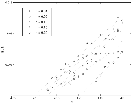
Figure 20: Freezing transition energies $e_{f}$, when using FMS. Each point corresponds to a single run ($N=10^{5}$). Dotted lines are linear fits.

In Figure 20 we present estimates of the freezing transition energy density $e_{f}\equiv E_{f}/N$ for a few sample runs of the FMS algorithm. We have not studied the dependence of $E_{f}$ on N, but it appears to be self-averaging, so that for any $\alpha$ and $\eta$ for which a freezing transition occurs, $e_{f}$ converges to a constant value as $N\to\infty$. Hence the $e_{f}$ values given in Figures 20 and 21 are similar to their $N\to\infty$ limits. Also the freezing transition time $t_{f}$ (measured in flips/$N$) seems to converge for many $(\alpha,\eta)$-pairs, but it is not at all clear that this needs to be so in every case. There may exist some region of $\alpha$ and $\eta$ values for which a superlinear number of flips are required before either a satisfying solution or a truth assignment with a core is reached (cf. Figure 22).

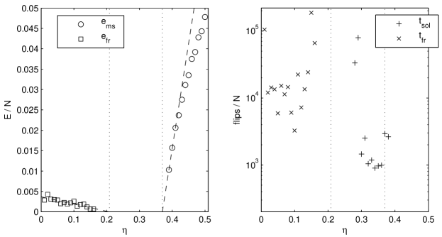
Figure 21: Sample runs of FMS at $\alpha=4.15$ ($N=10^{5}$). Left: Metastable energies and freezing transition energies. Right: Solution times and freezing transition times. Dotted lines give a rough estimate of the $(\eta_{l},\eta_{u})$-window at this $\alpha$.

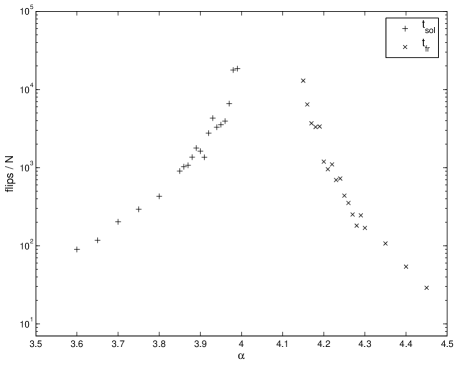
Figure 22: Solution times and freezing times, when using FMS with $\eta=0.05$. Each point corresponds to a single run ($N=10^{5}$).

We conjecture that there are almost always truth assignments with a core at all energy levels below any level at which a freezing transition can happen at given $\alpha$. For example, this implies that one can pick an $\eta$-value for $\alpha=4.2$, such that the freezing takes place at, say, $E/N=0.005$ (Figure 20). Hence we believe that there exist solutions with a core also in the $N\to\infty$ limit in some region of $\alpha$-values, approximately $4.10\lesssim\alpha<\alpha_{c}$. The lower bound of 4.10 has been estimated using FMS with $\eta=0.01$ (Figure 20). Since the choice of algorithm may have an effect on the estimate, the actual threshold point below which there do not exist solutions with a core in the $N\to\infty$ limit can be lower than this.

There may be a narrow region below $\alpha_{c}$ where typical instances do not have any completely white solutions. In this region, if it exists, focused algorithms presumably cannot find a solution in linear time. On the other hand, in MaMW04 it is conjectured that almost all solutions are completely white (“all-$*$ assignments” in the terminology of MaMW04 ) up to $\alpha_{c}$. This claim is based on experimental evidence using the survey propagation algorithm BrMZ02 ; MeZe02 ; BrZ03 , which seemingly finds only completely white solutions when N is large MaMW04 , just like focused local algorithms. However, if solutions with a core cannot be found in linear time, it is not surprising that usually the first solution encountered is completely white. Thus, the issue of a possible core transition (similar to the simpler XORSAT problem MeRZ03 ) below $\alpha_{c}$ remains open. We have not tried to assess which type of solution is more numerous near $\alpha_{c}$, or whether having a majority of completely white solutions is in fact a necessary or even a sufficient condition for maintaining time-linearity of local search methods. Thus, we can at the moment only conjecture a relation between the algorithmic performance of local search methods and the entropy of the solution space, as measured in terms of the “white” and “core” fractions vs. $N$.

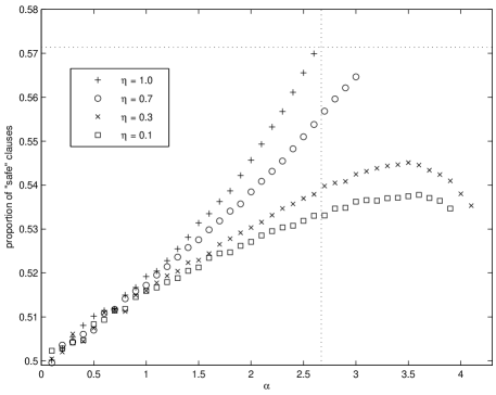
Figure 23: Proportion of “safe” clauses in solutions found by FMS. Each point corresponds to a single run ($N=10^{6}$). Horizontal dotted line is this proportion, when all the satisfying combinations have equal probability: $4/7$. Vertical dotted line is our estimate for the dynamical threshold of the Random Walk: $\alpha\approx 2.67$.

Another way to establish the existence of qualitatively different kinds of solutions is to look at the proportion of “safe” clauses (i.e. clauses that contain at least two satisfying literals) in the solutions found by FMS with different values of $\eta$ (Figure 23). One can say that with greater $\eta$, better quality solutions are found. Note that these safe clauses are just what enable variables to become unfrozen in the whitening algorithm (Figure 19).

Whiteness is just one indicator that can be used during the search process to tell when the linear-time property has been lost. Certainly there can be more powerful indicators that alarm about difficulties earlier, when the freezing transition has not yet happened. If a truth assignment which is not a solution is completely white, it means that any one of the still remaining unsat clauses can be resolved locally (assuming dependency loops between clauses don’t incidentally block this). It does not, however, mean that an arbitrary subset of the remaining unsat clauses could necessarily be resolved locally, or that there necessarily exists a solution. A truth assignment can turn from a completely white one to having a core by the flip of just one variable. One can envision higher order whitenings: a $k$th order whitening would tell whether all truth assigments that differ in at most $k$ variable values from the assignment in question are completely white (in the usual sense, i.e. zeroth order whitened). Maybe a higher order whitening with any fixed $k$ can (in principle) be used as an indicator for the linear-time property, just like the zeroth order one. There can also be some indicators that have nothing to do with whitening.

VI Conclusions

In this paper we have elucidated the behaviour of “focused” local search algorithms for the random 3-SAT problem. An expected conclusion is that they can be tuned so as to extend the regime of “good”, linear-in-N behaviour closer to $\alpha_{c}$.

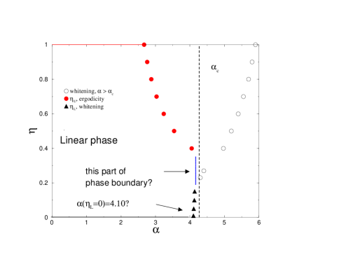
Figure 24: Proposed phase diagram for FMS. Above a dynamical threshold a metastable state is encountered before a solution is reached. Below a whitening threshold a freezing transition happens before a solution or a metastable or stable state is reached. The data points are rough estimates based on a few runs of the FMS algorithm.

An unexpected conclusion is that FMS (and WalkSAT, and FRRT) seem to work well very close to the critical threshold. Figure 24 proposes a phase diagram. FMS with $\eta=1$ is just the Random Walk algorithm; hence the first transition point is at $\alpha\approx 2.67$. For larger $\alpha$ there is the possibility of having two phase boundaries in terms of the noise parameter. The upper value $\eta_{u}$ separates the linear regime from one with too much noise, in which the fluctuations of the algorithm degrade its performance. For $\eta<\eta_{l}$, greediness leads to dynamical freezing, and though FMS (in contrast to FRRT in particular) remains ergodic, or able to climb out of local minima, the algorithm no longer scales linearly in the number of variables.

The phase diagram presents us with two main questions: what is the smallest $\alpha$ at which $\eta_{l}(\alpha)$ starts to deviate from zero? Does the choice of an ideal $\eta_{opt}$ allow one to push the linear regime arbitrarily close to $\alpha_{c}$? Note that the deviation of $\eta_{u}(\alpha)$ from unity with increasing $\alpha$ could perhaps be analysed with similar techniques as the methods in refs. BaHW03 ; SeMo03 . The essential idea there is to construct rate equations for densities of variables or clauses while ignoring correlations of neighboring ones. This would not resolve the above two main ones, of course.

The resolution of these questions will depend on our understanding the performance of FMS or other local search presence of the clustering of solutions. The whitening or freezing experiments provide qualitative understanding on the behaviour for small $\eta$: too greedy search procedures are not a good idea. Thus FMS seems to work well only when it actually finds solutions that can be completely whitened. Figure 24 also points out, via the whitening data for $\alpha>\alpha_{c}$, that the line of whitening thresholds $\eta_{l}$ for FMS apparently is continuous over $\alpha_{c}$. In particular in this case, one can then separate between two possible scenarios: either the $\eta_{u}$-line extends to $\alpha_{c}$ and finishes there, or otherwise it meets with the $\eta_{l}$-line at an $\alpha<\alpha_{c}$ at a point that is “tri-critical” in statistical mechanics terms. Note, however, that $\eta_{l}$ determined by whitening is not necessarily the highest lower bound to the linear phase.

The range of the algorithm presents therefore us with a fundamental question: though replica-methods have revealed the presence of clustering in the solution space starting from $\alpha\approx 3.92$, the FMS works for much higher $\alpha$’s still. The clustered solutions should have an extensive core of frozen variables, and therefore to be hard to find. Thus, the existence of “easy solutions” for the FMS tells that there are features in the solution space and energy landscape that are not well understood, since the FMS can pick, for a right choice of $\eta$ almost always such easy solutions out of those available for any particular instance. This would seem to imply that such completely white ones have a considerable entropy.

Our numerics also implies that in the linear scaling regime the solution time probability distributions become sharper (“concentrate”) as $N$ increases, implying indeed that the median solution time scales linearly. We can by numerical experiments not prove that this holds also for the average behaviour, but would like to note that the empirically observed tail behaviours for the same distributions give no indication of such heavy tails that would contradict this idea.

Acknowledgements: research supported by the Academy of Finland, Grants 206235 (S. Seitz) and 204156 (P. Orponen), and by the Center of Excellence program of the A. of F. (MA, SS) The authors would like to thank Dr. Supriya Krishnamurthy for useful comments and discussions.

References

- (1) E. Aarts and J. K. Lenstra (Eds.), Local Search for Combinatorial Optimization. J. Wiley & Sons, New York NY, 1997.
- (2) E. Aurell, U. Gordon and S. Kirkpatrick, Comparing beliefs, surveys and random walks. Technical report cond-mat/0406217, arXiv.org (June 2004).
- (3) W. Barthel, A. K. Hartmann and M. Weigt, Solving satisfiability problems by fluctuations: The dynamics of stochastic local search algorithms. Phys. Rev. E 67 (2003), 066104.
- (4) A. Braunstein, M. Mézard and R. Zecchina, Survey propagation: an algorithm for satisfiability. Technical report cs.CC/0212002, arXiv.org (Dec. 2002).
- (5) A. Braunstein and R. Zecchina, Survey propagation as local equilibrium equations, Technical report cond-mat/0312483, arXiv.org (Dec. 2003).
- (6) D. Du, J. Gu, P. Pardalos (Eds.), Satisfiability Problem: Theory and Applications. DIMACS Series in Discr. Math. and Theoret. Comput. Sci. 35, American Math. Soc., Providence RI, 1997.
- (7) G. Dueck, New optimization heuristics: the great deluge algorithm and the record-to-record travel. J. Comput. Phys. 104 (1993), 86–92.
- (8) M. R. Garey and D. S. Johnson, Computers and Intractability: A Guide to the Theory of NP-Completeness. W. H. Freeman & Co., San Francisco CA, 1979.
- (9) J. Gu, Efficient local search for very large-scale satisfiability problems. SIGART Bulletin 3:1 (1992), 8–12.
- (10) H. H. Hoos, An adaptive noise mechanism for WalkSAT. Proc. 18th Natl. Conf. on Artificial Intelligence (AAAI-02), 655–660. AAAI Press, San Jose Ca, 2002.
- (11) H. H. Hoos and T. Stützle, Towards a characterisation of the behaviour of stochastic local search algorithms for SAT. Artificial Intelligence 112 (1999), 213–232.
- (12) E. Maneva, E. Mossel and M. J. Wainwright, A new look at survey propagation and its generalizations. Technical report cs.CC/0409012, arXiv.org (April 2004).
- (13) N. Metropolis, A. Rosenbluth, M. Rosenbluth, A. Teller and E. Teller, Equations of state calculations by fast computing machines, J. Chem. Phys. 21 (1953), 1087–1092.
- (14) M. Mézard, F. Ricci-Tersenghi, and R. Zecchina, Alternative solutions to diluted p-spin models and XORSAT problems. J. Stat. Phys. 111 (2003), 505–533.
- (15) M. Mézard and R. Zecchina, Random K-satisfiability problem: From an analytic solution to an efficient algorithm. Phys. Rev. E 66 (2002), 056126.
- (16) D. Mitchell, B. Selman and H. Levesque, Hard and easy distributions of SAT problems. Proc. 10th Natl. Conf. on Artificial Intelligence (AAAI-92), 459–465. AAAI Press, San Jose CA, 1992.
- (17) A. Montanari, G. Parisi and F. Ricci-Tersenghi, Instability of one-step replica-symmetry-broken phase in satisfiability problems. J. Phys. A 37 (2004), 2073–2091.
- (18) C.H. Papadimitriou, On selecting a satisfying truth assignment. Proc. 32nd IEEE Symposium on the Foundations of Computer Science (FOCS-91), 163–169. IEEE Computer Society, New York NY, 1991.
- (19) G. Parisi, On local equilibrium equations for clustering states. Technical report cs.CC/0212047, arXiv.org (Feb 2002).
- (20) A. J. Parkes, Distributed local search, phase transitions, and polylog time. Proc. Workshop on Stochastic Search Algorithms, 17th International Joint Conference on Artificial Intelligence (IJCAI-01). 2001.
- (21) A. J. Parkes, Scaling properties of pure random walk on random 3-SAT. Proc. 8th Intl. Conf. on Principles and Practice of Constraint Programming (CP 2002), 708–713. Lecture Notes in Computer Science 2470. Springer-Verlag, Berlin 2002.
- (22) S. Seitz and P. Orponen, An efficient local search method for random 3-satisfiability. Proc. IEEE LICS’03 Workshop on Typical Case Complexity and Phase Transitions. Electronic Notes in Discrete Mathematics 16, Elsevier, Amsterdam2003.
- (23) B. Selman, H. Kautz, B. Cohen, Local search strategies for satisfiability testing. In: D. S. Johnson and M. A. Trick (Eds.), Cliques, Coloring, and Satisfiability, 521–532. DIMACS Series in Discr. Math. and Theoret. Comput. Sci. 26, American Math. Soc., Providence RI, 1996.
- (24) B. Selman, H. J. Levesque and D. G. Mitchell, A new method for solving hard satisfiability problems. Proc. 10th Natl. Conf. on Artificial Intelligence (AAAI-92), 440–446. AAAI Press, San Jose CA, 1992.
- (25) G. Semerjian and R. Monasson, Relaxation and metastability in a local search procedure for the random satisfiability problem. Phys. Rev. E 67 (2003), 066103.
- (26) G. Semerjian and R. Monasson, A study of Pure Random Walk on random satisfiability problems with “physical” methods. Proc. 6th Intl. Conf. on Theory and Applications of Satisfiability Testing (SAT 2003), 120–134. Lecture Notes in Computer Science 2919. Springer-Verlag, Berlin 2004.
- (27) W. Wei and B. Selman, Accelerating random walks. Proc. 8th Intl. Conf. on Principles and Practice of Constraint Programming (CP 2002), 216–232. Lecture Notes in Computer Science 2470. Springer-Verlag, Berlin 2002.