Scaling analysis of multivariate intermittent time series

Abstract

The scaling properties of the time series of asset prices and trading volumes of stock markets are analysed. It is shown that similarly to the asset prices, the trading volume data obey multi-scaling length-distribution of low-variability periods. In the case of asset prices, such scaling behaviour can be used for risk forecasts: the probability of observing next day a large price movement is (super-universally) inversely proportional to the length of the ongoing low-variability period. Finally, a method is devised for a multi-factor scaling analysis. We apply the simplest, two-factor model to equity index and trading volume time series.

,

1 Introduction

Predicting future developments of financial asset prices is an extremely difficult task. Certain problems, such as predicting the direction of movements, are nearly unsolvable. Meanwhile, certain aspects can be easily predicted. For instance, one can be sure that the prices will always fluctuate intermittently, largely due to people who believe they have found the winning algorithm, the philosopher’s stone.

The analysis of the historic charts of price dynamics is referred to as technical analysis [1]. The essence of the technical analysis is the hypothesis that the patterns of historic data can forecast the future price movements. On the other hand, the efficient market hypothesis (c.f. [2]) states that security prices reflect fully all available information. In its century-long history dated back to the work of Bachelier [3], the financial analysis has made use of the both approaches. The random walk hypothesis, standard deviation and the correlations between securities’ returns are the cornerstones of seminal papers in financial analysis [4, 5, 6]. Econophysics has introduced various more elaborate, mostly non-linear tools of analysis (c.f. [7, 8] and references therein). Here we extend a recently developed technique of length-distribution of low-variability periods [9].

Strongly non-linear systems, such as turbulent fluids and plasmas, granular media, biological and economical systems, etc., are typically characterized by scale-invariance and scaling laws. So, it should be not surprising that such seemingly different disciplines like turbulence studies, biological physics, and econophysics have many common tools of data analysis. For example, power-law distributions were first used in economics [10] in the end of 19th century, and later found in a wide variety of systems (often referred to as the Zipf’s law), c.f. [11, 12, 13, 14]. Similarly, diverse systems are known to generate signals, which are self-affine, and hence, can be characterized by the Hurst exponent, c.f. [15]. Further, the stable Lévy distributions (c.f. [16]) have been found to be relevant to all the mention disciplines; about truncated Levy flights in econophysics, c.f. [17]. Finally, multi-fractal formalism is by far the most popular tool for scale-invariant analysis of intermittent time-series, c.f. [18, 19]. It should be noted, however, that in many cases (including econophysical applications), there is no profound understanding of the origin of multi-fractality, and hence, the multi-fractal analysis is not necessarily the optimal method. Indeed, multi-fractal formalism has been devised in the context of turbulence, and is specifically suited for systems with random multiplicative cascades [20]. Meanwhile, in the case of such time-series as stock prices or heart rate variability signal, the presence of multiplicative cascades is not evident.

Therefore, there is a clear need for a deeper understanding of the character of intermittency in the case of financial time-series. This problem can be approached by studying new independent and/or more general methods of scale-invariant analysis. For instance, in the case of heart rate variability, it has been found that the whole time-period can be clusterised into self-similarly distributed segments of approximately constant heart rate [21]. In order to address this problem, a new method has been suggested recently [9] which is based on the analysis of the distribution of low-variability periods. The low-variability period is defined as a time period with maximal length where consecutive relative changes in realizations of the time series are less than given threshold $\delta$. Note that in addition to the financial assets, the low-variability period analysis has been applied to biological systems [22, 23]. It has been shown [9] that in the case of the multi-affine time series, the cumulative distribution function of the low-variability periods is in the form of a (multi-scaling) power-law. Since the opposite is not necessarily true, the low-variability period analysis is, indeed, a more universal method than the multi-affine analysis.

Even if the time-series is actually multi-affine, the low-variability period analysis can be still useful, because (a) the power-law exponent is related to the multi-fractal dimension; this circumstance provides an easy method for checking the assumption of multi-affinity; (b) low-variability periods provide higher time-resolution of time series analysis [9].

This paper serves three main purposes. First, we are going to apply the method of the analysis of low-variability periods to the data of trading volumes. This analysis is motivated as follows. Similarly to the asset prices, the trading volumes are known to fluctuate intermittently, c.f. [24, 25]. According to the Mandelbrot’s model of stock prices as a fractional Brownian motion in multi-affine trading time [18], one could expect that the time series of trading volumes are multi-affine. The analysis of the length-distribution of low-variability periods of trading volumes serves as a test of this model. Second, we discuss the consequences of the presence of power laws of low-variability periods. Third, an attempt is made to generalize the method to multivariate time-series (e.g. a stock price together with the trading volume). It should be noted that in the case of multi-affine analysis, there is no simply interpretable way for such a generalization.

2 Scaling of trading volumes

We start with a brief description of the method devised in Ref. [9, 22], A low-variability period is defined as such a contiguous time-interval $T_{i}=[t_{i},t_{i}+l_{i}]$, which satisfies the conditions

$$|V(t)/\left<V(t)\right>_{\tau}-1|\leq\delta\;\;\mbox{for}\;\;t\in T_{i},$$ (1)

and $|V(t)/\left<V(t)\right>_{\tau}-1|>\delta$ for $t=t_{i}-1,t_{i}+l_{i}+1$; it is assumed that the data sampling interval serves as the time unit. The average of the trading volumes $V(t)$ is taken over a time window of length $\tau$:

$$\left<V(t)\right>_{\tau}=\frac{1}{\tau}\sum_{k=0}^{\tau-1}V(t-k).$$ (2)

Therefore, we have two control parameters: (i) $\tau$ — the length of the averaging window, and (ii) $\delta$ — the variability threshold. Further, the cumulative length-distribution function of low-variability periods $R(n)$ is introduced: $R(n)$ is the number of the low-variability periods of length $l_{i}\geq n$. We speak about multi-scaling behaviour, if the following power-law is observed:

$$R(n)=R_{0}n^{-\alpha(\delta,\tau)},$$ (3)

where $\alpha(\delta,\tau)$ is a scaling exponent and $R_{0}$ is a constant.

It has been shown [9] that in the case of multi-affine time-series, the low-variability periods do follow a multi-scaling distribution law:

$$\alpha(\delta,\tau)=f(\log_{\tau}\delta),$$ (4)

where $f(h)$ denotes the Hölder multifractal spectrum of the local Hurst exponents $h$. Meanwhile, the presence of a scaling law (3) does not necessarily imply multifractality. Indeed, note that the Hölder exponent $f(h)$ cannot exceed the topological dimensionality (one), therefore the values $\alpha>1$ are not related to multifractality. It should be stressed that unequality $\alpha(\delta,\tau)>1$ does neither imply the lack of multifractality: in the case of multi-fractal time-series, $\alpha(\delta,\tau)>1$ can (in principle) be observed for $\log_{\tau}\delta<h_{0}$, where $h_{0}$ is the dominant local Hurst exponent, $f(h_{0})=1$. For this range of parameters, the unequality $\alpha(\delta,\tau)>1$ must be satisfied (assuming that $\alpha$ is a monotonous function of $\delta$). Finally, if there is no data collapse $\alpha(\delta,\tau)\equiv f(\log_{\tau}\delta)$ for $\alpha(\delta,\tau)\leq 1$, the underlying time-series is certainly non-multifractal. In the case of currency rates, a reasonable data collapse [according to Eq. (4)] has been observed. In this Section, the daily trading volume data of various stock indices are tested for multi-scaling and multi-fractality.

2.1 The data and the calculations

The stock market volumes are measured in the amount of shares traded on the exchange. The data used in the analysis represent the daily closing prices and trading volumes and it is described in detail in the Table 1.

Table 1: The data used in volume analysis

Abbr	Description	Calendar Period	# of data
SPX	Standard & Poor’s 500 Index	04/01/93 - 13/09/04	2947
DAX	The German Stock Index	04/01/93 - 13/09/04	2950
NKY	Nikkei 225 Stock Average	04/01/93 - 14/09/04	2879
MXEA	The MSCI Europe, Australasia and Far East Index	04/06/01 - 13/09/04	832
CAC	CAC-40 Index of Paris Bourse	04/01/93 - 13/09/04	2953
UKX	FTSE 100 Index	04/01/93 - 13/09/04	2953
MXWO	MSCI World Index	04/01/01 - 13/09/04	809
INDU	Dow Jones Industrial Average	04/01/93 - 13/09/04	2941
TALSE	Tallinn Stock Exchange Index	25/02/03 - 13/09/04	392
RTS	Russian Trading System Index	03/07/01 - 13/09/04	794
WIG	Warsaw General Index	23/05/01 - 13/09/04	836
BUX	Budapest Stock Exchange Index	15/09/97 - 13/09/04	1747

If the cumulative distribution function $R(n)$ is plotted against $n$ in log-log scale, the power-law Eq. (3) corresponds to a straight line. The scaling exponent $\alpha(\delta,\tau)$ was found as the slope of the linear trend line in log-log space, using the least-square fit method.

The error of $\alpha(\delta,\tau)$ was estimated as follows: The least-squares fitted trend-line was found as described above, except that the slope $\alpha$ was not optimised, i.e. it was considered as a fixed parameter. Further, the sum of squared residuals $r(\alpha)$ was calculated as a function of $\alpha$. The error estimate was found as $e=(\alpha^{\prime}-\alpha)$, where $\alpha$ is the least-squares fitted value of the slope, and $\alpha^{\prime}$ satisfies the condition $r(\alpha^{\prime})=2r(\alpha)$.

We used $\delta=[5\%,10\%,...,70\%]$ and $\tau=[2,3,5,10]$ days as input parameters for all of the time series described in Table 1. Total 650 calculations were carried out and in most cases the least-square fit provided good results. The quality of the fit is measured by the $R^{2}$ coefficients that are plotted into the histogram in Fig 1. The scaling exponents (found with $\tau=10$ days) with error estimates are presented in Table 2.

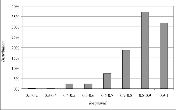
Figure 1: Histogram of R-squared coefficients based on the regression analysis of determining scaling exponent $\alpha(\delta,\tau)$

Table 2: The values of the scaling exponent $\alpha(\delta,\tau=10days$) in the case of daily trading volumes for various stock indices and different values of the parameter $\delta$

$\delta$(%)	CAC	DAX	INDU	NKY	SPX	UKX
5.0	3.49$\pm$0.45	3.71$\pm$0.33	3.39$\pm$0.40	3.16$\pm$0.30	3.55$\pm$0.46	3.65$\pm$0.39
10.0	3.34$\pm$0.47	3.21$\pm$0.35	2.63$\pm$0.33	3.01$\pm$0.43	2.75$\pm$0.32	2.94$\pm$0.28
15.0	2.89$\pm$0.39	2.61$\pm$0.28	2.25$\pm$0.19	2.78$\pm$0.42	2.13$\pm$0.26	2.73$\pm$0.27
20.0	2.63$\pm$0.27	2.44$\pm$0.37	1.90$\pm$0.15	2.07$\pm$0.27	1.95$\pm$0.23	2.50$\pm$0.30
25.0	2.44$\pm$0.23	2.33$\pm$0.37	1.79$\pm$0.22	2.00$\pm$0.18	1.68$\pm$0.14	1.97$\pm$0.24
30.0	2.34$\pm$0.26	1.71$\pm$0.23	1.69$\pm$0.24	1.70$\pm$0.16	1.37$\pm$0.15	1.83$\pm$0.19
35.0	1.99$\pm$0.23	1.58$\pm$0.26	1.65$\pm$0.19	1.36$\pm$0.13	1.14$\pm$0.12	1.52$\pm$0.15
40.0	1.66$\pm$0.19	1.62$\pm$0.20	1.24$\pm$0.14	1.49$\pm$0.18	1.10$\pm$0.10	1.38$\pm$0.17
45.0	1.78$\pm$0.20	1.42$\pm$0.17	1.12$\pm$0.16	1.39$\pm$0.21	0.98$\pm$0.11	1.05$\pm$0.17
50.0	1.55$\pm$0.20	1.44$\pm$0.20	1.44$\pm$0.13	1.67$\pm$0.19	0.82$\pm$0.09	1.20$\pm$0.13
55.0	1.35$\pm$0.16	1.32$\pm$0.19	1.21$\pm$0.11	1.56$\pm$0.17	0.80$\pm$0.09	0.96$\pm$0.11
60.0	1.41$\pm$0.20	1.22$\pm$0.15	1.11$\pm$0.12	1.47$\pm$0.16	0.55$\pm$0.08	0.94$\pm$0.12
65.0	1.15$\pm$0.15	1.01$\pm$0.15	0.98$\pm$0.13	1.42$\pm$0.13	0.77$\pm$0.08	0.86$\pm$0.13
70.0	1.37$\pm$0.19	0.91$\pm$0.14	0.98$\pm$0.12	1.25$\pm$0.10	0.71$\pm$0.07	0.89$\pm$0.14
$\delta$(%)	BUX	WIG	TALSE	RTSI	MXEA	MXWO
5.0	3.50$\pm$0.25	3.23$\pm$0.11	3.65$\pm$0.39	3.70$\pm$0.06	3.32$\pm$0.75	2.81$\pm$0.32
10.0	3.45$\pm$0.54	2.64$\pm$0.27	3.11$\pm$0.07	2.64$\pm$0.11	2.57$\pm$0.31	2.35$\pm$0.23
15.0	2.36$\pm$0.30	2.77$\pm$0.37	2.84$\pm$0.19	3.17$\pm$0.42	2.23$\pm$0.30	1.99$\pm$0.23
20.0	2.58$\pm$0.36	2.67$\pm$0.44	2.70$\pm$0.26	3.13$\pm$0.43	1.60$\pm$0.16	1.30$\pm$0.13
25.0	2.50$\pm$0.25	2.07$\pm$0.27	2.88$\pm$0.36	2.63$\pm$0.34	1.29$\pm$0.16	1.12$\pm$0.15
30.0	2.19$\pm$0.23	2.25$\pm$0.29	2.37$\pm$0.46	2.28$\pm$0.32	1.18$\pm$0.12	0.89$\pm$0.15
35.0	2.11$\pm$0.25	1.89$\pm$0.17	2.45$\pm$0.34	2.05$\pm$0.22	1.12$\pm$0.14	1.01$\pm$0.15
40.0	1.97$\pm$0.15	1.57$\pm$0.13	2.04$\pm$0.28	1.89$\pm$0.31	0.89$\pm$0.09	0.63$\pm$0.07
45.0	1.89$\pm$0.14	1.47$\pm$0.10	2.02$\pm$0.32	2.01$\pm$0.30	0.67$\pm$0.08	0.63$\pm$0.08
50.0	1.81$\pm$0.16	1.31$\pm$0.12	1.95$\pm$0.26	1.97$\pm$0.20	0.57$\pm$0.07	0.63$\pm$0.07
55.0	1.65$\pm$0.14	1.37$\pm$0.10	1.59$\pm$0.17	1.64$\pm$0.14	0.64$\pm$0.08	0.56$\pm$0.09
60.0	1.51$\pm$0.16	1.38$\pm$0.12	1.64$\pm$0.19	1.46$\pm$0.17	0.51$\pm$0.10	0.56$\pm$0.09
65.0	1.36$\pm$0.16	1.21$\pm$0.12	1.60$\pm$0.22	1.36$\pm$0.19	0.51$\pm$0.10	0.53$\pm$0.09
70.0	1.28$\pm$0.16	1.22$\pm$0.11	1.33$\pm$0.18	1.28$\pm$0.21	0.37$\pm$0.06	0.33$\pm$0.07

2.2 Scaling properties of volume data and discussions

As seen from Fig. 1 and Table 2, the low-variability periods of the daily volume time series follow reasonably well a multi-scaling behaviour (similarly to what has been observed in the case of stock prices [9]). In Fig. 2, the scaling exponent $\alpha(\delta,\tau)$ is plotted against the $log_{\tau}\delta$ for DAX and SPX time series with $\tau=3,5,10$ days. We can see that there is a departure from the multi-affine expectation — there is no data collapse at range $\alpha\leq 1$ [which would have been corresponding to Eq. (4)]. This observation is interpreted as follows. Here, each data point describes the amount of shares traded in respective stock exchange in a calendar day. The condition $\alpha<1$ is satisfied only for very high thresholds ($\delta>50\%$). Typically, there are very few periods, when trading volumes would fluctuate with such a large amplitude. Therefore, the number of valid data points is very low. As a consequence, the scaling range is narrow, and the formally calculated scaling exponent is non-stationary (depends on the particular realisation of the time-series). This behaviour is different from what has been observed for currency time series (when the results $\alpha\leq 1$ were more stationary, with a reasonable data collapse in $\alpha-\log_{\tau}\delta$-plot).

So, we can conclude that while the trading volume data are intermittent and fluctuations are scale-invariant [described by Eq. (3)], the degree of intermittency is lower than in the case of currency fluctuations: the scaling exponent values tend to be always larger than one. Respectively, the multifractal pattern [like described by Eq. (4)] is not observable.

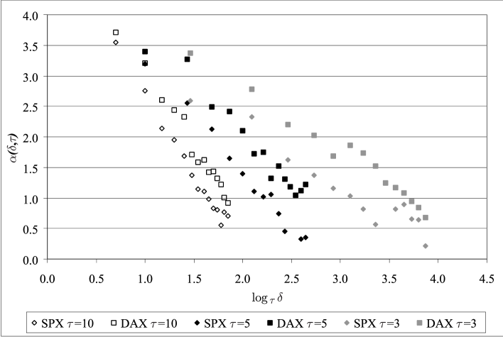
Figure 2: Scaling exponent $\alpha(\delta,\tau)$ plotted against $log_{\tau}\delta$ for SPX and DAX time series for $\tau=3,5,10$ days

2.3 Consequences of the scaling behaviour

In the case of financial time-series, a crucial question is how to make forecasts. The most useful kind of forecasts would give predictions of the direction of future prices. However, these forecasts will be always very unreliable, the efficient market hypothesis denies such a possibility entirely (c.f. second law of thermodynamics). Meanwhile, the risk-related forecasts are completely possible (and may prove to be useful). Therefore, a natural question arises: what are the risk-prediction-related consequences of the presence of the power-law distribution of low-variability periods? More specifically, suppose we have had a low-variability period, which had lasted $n$ days (and still goes on). Can we say something about the possibility of today being the last day of this “silent” period? In other words, what is the probability $p(n)$ that the tomorrow’s movement exceeds our pre-fixed threshold $\delta$?

Apparently, this probability is given by the ratio of (a) the number of those low-variability periods, the length of which is exactly $n$, $N_{a}=R(n)-R(n+1)$, and (b) the number of those low-variability periods, which have length $m\geq n$, $N_{b}=R(n)$. If $n$ is large, the difference $R(n)-R(n+1)$ can be calculated approximately as $-\frac{dR}{dn}$. Upon applying Eq. (3) we arrive at $N_{a}\approx\alpha R_{0}n^{-\alpha-1}$ and $N_{b}\approx R_{0}n^{-\alpha}$. Bearing in mind that $p(n)=N_{a}/N_{b}$, the final result is written as

$$p(n)\approx\alpha n^{-1}.$$ (5)

Therefore, we have shown that the very presence of a power law of the low-variability periods has an interesting consequence: the probability that the tomorrow’s price movement will be larger than the movements of $n$ preceding days, is inversely proportional to $n$. The predicted power law exponent is independent of the scaling exponent $\alpha(\delta,\tau)$, i.e. we are dealing with super-universality. This super-universality appears to be related to the super-universality of the scaling of direct avalanches in self-organised critical systems [26]. It allows us to make every day a series of forecasts: by scanning the values of the threshold parameter $\delta$, we find the length $n_{\delta}$ of the current (still ongoing) low-variability period. Then, the probability that the tomorrow’s movement $p(\delta)$ remains below the threshold $\delta$ is estimated as $p(\delta)\approx\alpha(\delta,\tau=2\,\mbox{days})n_{\delta}^{-1}$. Note that the prefactor $\alpha(\delta,\tau=2\,\mbox{days})\approx 1$ can be dropped, but will improve the forecast; $\tau=2$ days means that only the prices of two subsequent days are compared.

3 Two-factor model of scale invariance in financial time series

In the technical analysis, various forms of multi-factor models have been used for some time [1]. In particular, it has been conjectured that in the case of trading volumes and price fluctuations, the higher-than average trading volumes generally “confirm” the price trend. However, according to our best knowledge, scale-invariant methods have not yet been applied to the multi-factor studies.

The low-variability period analysis provides simply interpretable way of generalisation of multi-signal time series analysis. With the conventional multi-affine analysis, the interpretation of the results is significantly harder. Indeed, consider the wavelet transform $w(a,b)$, where $a$ denotes a coordinate and $b$ stands for the wavelet width. For a multi-affine signal, the following scaling law is expected: $\left<w(a,b)^{q}\right>\propto b^{\tau_{q}}$. For a bi-variate analysis of two signals, this equation can be generalized as $\left<w_{1}(a,b)^{q}\cdot w_{2}(a,b)^{p}\right>\propto b^{\tau_{q,p}}$. Here, $w_{1}$ and $w_{2}$ denote the wavelet transform of the two signals. For two dependent signals, $\left<w_{1}(a,b)^{q}\cdot w_{2}(a,b)^{p}\right>\neq\left<w_{1}(a,b)^{q}\right>\cdot\left<w_{2}(a,b)^{p}\right>$; however, there is no clear way of interpreting the features of the scaling exponent $\tau_{q,p}$. Therefore, in this section, the analysis of low-variability periods is generalised and the multi-factor model is proposed. In particular, we address the above mentioned statement about the relationship between trading volumes and stock prices.

In our previous calculations, the low-variability periods are defined either via the condition (1), or via the same unequality, with trading volume $V(t)$ being substituted by stock price (or index value) $p(t)$ [9]:

$$|p(t)/\left<p(t)\right>_{\tau}-1|\leq\delta_{p}\;\;\mbox{for}\;\;t\in T_{i}.$$ (6)

Hereinafter we refer to the application of Eq. (6) as the usage of the single-factor price model or Method 0 (for brevity). Similarly, the condition (1) corresponds to the single-factor volume model or Method 0 (Volume). There are two ways to generalize the concept of low-variability into multi-factor model:

1. Low-variability persists if both condition (1) and (6) are satisfied;

2. Low-variability persists if any of the conditions (1) and (6) are satisfied.

It is clear that the number of low-variability periods is larger by using the latter option. In fact, using the first option led us often to a very small number of low-variability periods (this, of course, is related to the limited length of the time-series). Therefore, here we present only the results corresponding to the second definition. Note that for multi-factor models with more than two inputs, the conditions similar to Eq. (6) can be combined with any set of logical operators “and” and “or”.

In what follows we use several definitions of the two-factor low-variability periods (the application of these definitions will be referred to as Method 1 – Method 3, respectively):

$$(|p(t)/\left<p(t)\right>_{\tau}-1|\leq\delta_{p})\bigvee(|V(t)/\left<V(t)\right>_{\tau}-1|\leq\delta_{v})\;\;\mbox{for}\;\;t\in T_{i}.$$ (7)

$$(|p(t)/\left<p(t)\right>_{\tau}-1|\leq\delta_{p})\bigvee(V(t)/\left<V(t)\right>_{\tau}-1\leq\delta_{v})\;\;\mbox{for}\;\;t\in T_{i}.$$ (8)

$$(|p(t)/\left<p(t)\right>_{\tau}-1|\leq\delta_{p})\bigvee(V(t)/\left<V(t)\right>_{\tau}-1\geq-\delta_{v})\;\;\mbox{for}\;\;t\in T_{i}.$$ (9)

3.1 Asymptotic behaviour

Equation (7) is symmetric with respect to the price and volume conditions. The low-variability period is terminated as soon as the relative price change exceeds (by modulus) $\delta_{p}$, and the relative volume change exceeds (by modulus) $\delta_{v}$.

If the condition (7) is applied, the following asymptotic laws are expected:

$$\alpha(\delta_{p},\delta_{V},\tau)\to\alpha(\delta_{p},\tau)\;\;\mbox{when}\;\;\delta_{V}\to 0,$$

and

$$\alpha(\delta_{p},\delta_{V},\tau)\to\alpha(\delta_{V},\tau)\;\;\mbox{when}\;\;\delta_{p}\to 0.$$

Such a behaviour is, indeed, observed for the time series of DAX and SPX. The data used in the calculations is described in Table 1. In Figures 3 and 4 the scaling exponents $\alpha(\delta_{p},\delta_{V},\tau)$ are displayed for DAX and SPX time series by using $\tau=10$ days. ¿From Fig. 3, it is seen that for low values of $\delta_{V}$, the low-variability condition for volume is almost always violated. Therefore, the scaling exponent is defined almost solely with the price parameter (the curves with $\delta_{V}=0$ and $\delta_{V}=0.5$ are very close to each other). On the other hand, for high values of $\delta_{V}$, the volume condition is typically satisfied, and the horizontal lines (in $\alpha$-$\delta_{p}$ space) denote a low dependence on the price parameter. These arguments apply to the dependence of the exponent $\alpha(\delta_{p},\delta_{V},\tau)$ on the price threshold parameters, as well, see Fig. 4.

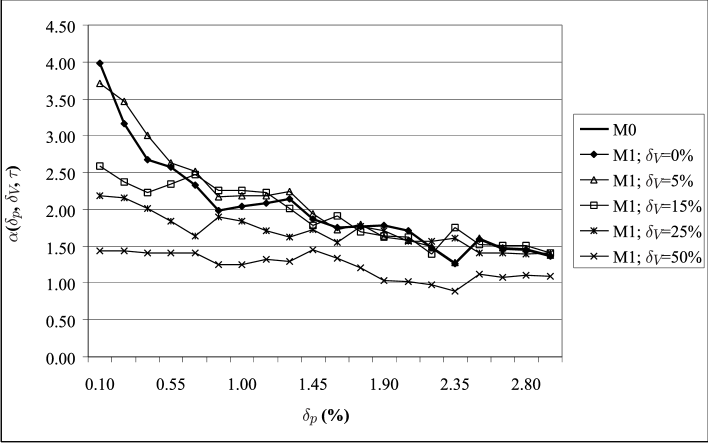
Figure 3: The convergence of Method 1 $\to$ Method 0. The scaling exponents $\alpha(\delta_{p},\delta_{V},\tau)$ are calculated for DAX time series by using conditions (6) and (7) with $\tau=10$ days and $\delta_{v}=[50\%,25\%,15\%,5\%,0\%]$

.

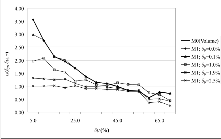
Figure 4: The convergence of Method 1 $\to$ Method 0 (Volume). The scaling exponents $\alpha(\delta_{p},\delta_{V},\tau)$ are calculated for SPX time series by using conditions (1) and (7) with $\tau=10$ days and $\delta_{p}=[2.5\%,1.9\%,1.0\%,0.1\%,0.0\%]$

.

3.2 Methods 2 and 3: differences between volume spike and volume squeeze

According to Eq. (8), the low-variability period is terminated when price change (rise or drop) is significant (i.e. larger than the threshold parameter), and the volume increases faster than the threshold. Equation (9) represents a definition, opposite to Eq. (8): the low-variability period is terminated when the price change exceeds the threshold parameter, and the volume decreases faster than the threshold. These definitions are useful for studying the asymmetry between the volume rise and drop: if the multi-scaling exponent $\alpha(\delta_{p},\delta_{V},\tau)$ turns out to be different for Methods 2 and 3, there must be an asymmetry between those volume spike and squeeze events, which are accompanied by a large price variability. Indeed, the price condition in Eqns (8) and (9) is the same; so, the differences in the scaling exponent $\alpha(\delta_{p},\delta_{V},\tau)$ must be due to the different effect of the volume condition (8) and (9).

Let us refer back to Method 1 [Eq. (7)]. With this method, the events terminating the low-variability periods represent a superposition of the respective events for the Methods 2 and 3 [Eqns (8) and (9)]. So, if the scaling exponents calculated according to Method 2 are very similar to the ones calculated according to Method 1, we can conclude, that the amount of the low-variability periods defined by Method 3 is insignificant. The same holds true if the scaling exponents of Method 3 tend to be similar to the ones of Method 1.

The multi-factor scaling exponents $\alpha(\delta_{p},\delta_{V},\tau)$ are found for the DAX data with $\tau=10$ days. In Fig. 5, the scaling exponents $\alpha(\delta_{p},\delta_{V},\tau=10)$ of DAX index are plotted against $log_{\tau=10}\delta_{p}$ with (a) $\delta_{V}=5\%$, (b) $\delta_{V}=15\%$, (c) $\delta_{V}=25\%$ and (d) $\delta_{V}=50\%$ . The Methods 0-3 [Eqns (6)–(9)] are used for definition of low-variability periods.

Figure 5: Multi-affine scaling of the two-factor model. The scaling exponents $\alpha(\delta_{p},\delta_{V},\tau)$ of DAX time series are plotted against $log_{\tau=10}\delta_{p}$ with (a) $\delta_{V}=5\%$, (b) $\delta_{V}=15\%$, (c) $\delta_{V}=25\%$ and (d) $\delta_{V}=50\%$

3.3 Discussion of the results

By giving a small value to the thresholds $\delta_{V}$ and $\delta_{p}$ in any of Eqns (6)–(9), the number of longer low-variability periods becomes small. Therefore, we have a large number of short low-variability periods (compared to high $\delta$ values); this leads to high values of the scaling exponent. In Fig. 5a, the threshold value of $\delta_{V}$ is set to very low level of $5\%$. From Eq. (7) it can be seen that then the two-factor model leads to results which are very similar to the single-factor (i.e. price factor) model. Likewise, the larger the volume threshold $\delta_{V}$, the larger the difference between the $\alpha$–$\delta_{p}$-curves of the single- and multi-factor models (at $\delta_{V}=50\%$, the curves are rather dissimilar).

An important issue is the difference between the curves of Methods 2 and 3. One can notice that there is a different behaviour at the small values of the parameter $\delta_{p}$, an evidence of the asymmetry between volume rise and drop. One can also notice that the scaling exponents calculated according to the Method 3 [Eq. (9)] are lower than the ones calculated according to Methods 1 and 2 [Eqns (7) and (8)]. Meanwhile, the difference between the outcomes of the Methods 1 and 2 [Eqns (7) and (8)] is minor. Therefore, we conclude, that high price variability is typically accompanied by increasing volume. This conclusion is independent of the price/volume pre-history (i.e. is valid both for short and long low-variability periods).

In this paper, we have not analysed the problem of higher-rank multi-factor models. However, this can be useful for e.g. multi-stock data analysis, where each stock price provides an independent input stream. This situation will be addressed in further studies.

4 Conclusion

The concept of low-variability periods has been proven to be useful for various econophysical issues (not just limited to the scope of stock prices/indices and currency exchange rates). So, we found that the time series of stock trading volumes obey multi-scaling properties, similarly like the price data. However, while the multi-scaling exponent of the price time series follows a pattern, characteristic to the multi-affine data, in the case of trading volumes, there is a clear departure from that pattern (one can say that the fluctuations are less intermittent).

Further, we have shown that the presence of the multi-scaling distribution of the length-distribution of the low-variability periods gives rise to a super-universal scaling law for the probability of observing next day a large price movement. This probability is inversely proportional to the length of the ongoing low-variability period, a fact which can be used for risk forecasts.

Finally, the multi-factor model is proposed for time series analysis. In this paper, only the simplest two-factor model is described and applied to stock price and volume data. The low-variability periods of multi-variate time series can be defined in different ways; for instance, the threshold conditions applied to the single data streams can be combined by logical “and”, as well as by logical “or”. In the our case of price and volume data, three different definitions of low-variability periods have been applied (in order to study the asymmetry between the volume rise and drop, we have also applied sign-dependant threshold conditions). This analysis led us to the conclusion that high price variability is typically accompanied by increasing trade volume, independently of the prior events of the market. In the light of this observation, the common thesis of technical analysis, “increased trading volumes confirms the price trend”, becomes less useful. Indeed, most of the significant price jumps are accompanied by increased trading volumes; so, almost all the “price trends” pretend to be “confirmed”.

References

- [1] J. Murphy, Technical analysis of the futures markets, New York Institute of Finance, New York, 1986
- [2] E. Fama, Journal of Business 38 (1965) 34E. Fama, Journal of Finance 25 (1970) 383E. Fama, Journal of Finance 46 (1991) 1575
- [3] L. Bachelier, Theorie de la speculation. (Doctoral dissertation in Mathematical Sciences, Faculte des Sciences de Paris, defended March 19, 1900
- [4] H. Markowitz, Journal of Finance 7 (1952) 77
- [5] W. Sharpe, Journal of Finance 19 (1964) 425
- [6] F. Black, M. Scholes, Journal of Political Economy 81 (1973) 637
- [7] R.N. Mantegna, H.E. Stanley, An Introduction to Econophysics: Correlations and Complexity in Finance, Cambridge University Press, Cambridge, 1999
- [8] J. Voit, The Statistical Mechanics of Financial Markets, Springer-Verlag, Berlin Heidelberg, 2001
- [9] R. Kitt, J. Kalda, Physica A 345 (2005) 622
- [10] V. Pareto, Le Cours d’ Economie Politique, Lausanne Paris, 1897
- [11] G.K. Zipf, Human Behavior and the Principle of Least Effort, Cambridge, Addison-Wesley, 1949
- [12] M. Ausloos, Ph. Bronlet, Physica A 324 (2003) 30
- [13] X. Gabaix, P. Gopikrishnan, V. Plerou and H.E. Stanley, Nature 423 (2003) 267Xavier Gabaix, Power laws and the origins of the business cycle, MIT, Department of Economics and NBER, August 20, 2003
- [14] Y. Fujiwara, C. Di Guilmi, H. Aoyama, M. Gallegati, W. Souma, Physica A 335 (2004) 197Y. Fujiwara, Physica A 337 (2004) 219
- [15] B.B. Mandelbrot, The Fractal Geometry of Nature, W.H.Freeman, New York, 1982
- [16] M. Shlesinger, G. M. Zaslavsky, U. Frisch, Lévy Flights and Related Topics in Physics, Springer-Verlag, Berlin Heidelberg, 1995
- [17] R.N. Mantegna, H.E. Stanley, Phys. Rev. Lett. 73 (1994) 2946
- [18] B.B. Mandelbrot, Fractals and Scaling in Finance: Discontinuity, Concentration, Risk. Springer, Berlin 1997
- [19] N. Vandewalle, M. Ausloos, Eur. Phys. J. B 4 (1998) 257
- [20] R. Benzi, G. Paladin and A. Vulpiani and M. Vergassola, J. Phys. A: Math 17 (1984) 3521
- [21] P. Bernaola-Galván, P.Ch. Ivanov, L.A.N. Amaral and H.E. Stanley, Phys. Rev. Lett. 87 (2001) 168105
- [22] J. Kalda, M. Säkki, M. Vainu, M. Laan, arXiv:physics/0110075 v1 26 Oct 2001, M.Säkki, J. Kalda, M. Vainu, M. Laan, Physica A 338 (2004) 255
- [23] M. Bachmann, J. Kalda, J. Lass, V. Tuulik, M. Säkki, H. Hinrikus, Method of nonlinear analysis of electroencephalogram for detection of the effect of low-level electromagnetic field, Accepted (2004) by: Med. Biol. Eng. Comput.
- [24] P. Gopikrishnan, V. Plerou, X. Gabaix, H.E. Stanley, Phys. Rev. E 62 (2000) 4493
- [25] M. Ausloos, K. Ivanova, in: H. Takayasu (Ed.), The applications of econophysics, Proceedings of the Second Nikkei Econophysics Symposium, Springer Verlag, Berlin, 2004, p. 117
- [26] S. Maslov, Phys. Rev. Lett. 74 (1995) 562