Thermal noise properties of two aging materials

Abstract

In this lecture we review several aspects of the thermal noise properties in two aging materials: a polymer and a colloidal glass. The measurements have been performed after a quench for the polymer and during the transition from a fluid-like to a solid-like state for the gel. Two kind of noise has been measured: the electrical noise and the mechanical noise. For both materials we have observed that the electric noise is characterized by a strong intermittency, which induces a large violation of the Fluctuation Dissipation Theorem (FDT) during the aging time, and may persist for several hours at low frequency. The statistics of these intermittent signals and their dependance on the quench speed for the polymer or on sample concentration for the gel are studied. The results are in a qualitative agreement with recent models of aging, that predict an intermittent dynamics. For the mechanical noise the results are unclear. In the polymer the mechanical thermal noise is still intermittent whereas for the gel the violation of FDT, if it exists, is extremely small.

1 Introduction

When a glassy system is quenched from above to below the glass transition temperature $T_{g}$, any response function of the material depends on the time $t_{w}$ elapsed from the quench[1]. For example, the dielectric and elastic constants of polymers continue to evolve several years after the quench [1]. Similarly, the magnetic susceptibility of spin-glasses depends on the time spent at low temperature [2]. Another example of aging is given by colloidal-glasses, whose properties evolve during the sol-gel transition which may last a few days [3]. For obvious reasons related to applications, aging has been mainly characterized by the study of the slow time evolution of response functions, such as the dielectric and elastic properties of these materials. It has been observed that these systems may present very complex effects, such as memory and rejuvenation[1, 4, 5, 6], in other words their physical properties depend on the whole thermal history of the sample. Many models and theories have been constructed in order to explain the observed phenomenology, which is not yet completely understood. These models either predict or assume very different dynamical behaviours of the systems during aging. This dynamical behaviour can be directly related to the thermal noise features of these aging systems and the study of response functions alone is unable to give definitive answers on the approaches that are the most adapted to explain the aging of a specific material. Thus it is important to associate the measure of thermal noise to that of response functions. The measurement of fluctuations is also related to another important aspect of aging dynamics. Indeed glasses are out of equilibrium systems and usual thermodynamics does not necessarily apply. However, as the time evolution is slow, some concepts of the classical approach may be useful for understanding the glass aging properties. A widely studied question is the definition of an effective temperature in these systems which are weakly, but durably, out of equilibrium. Recent theories[7] based on the description of spin glasses by a mean field approach proposed to extend the concept of temperature using a Fluctuation Dissipation Relation (FDR) which generalizes the Fluctuation Dissipation Theorem (FDT) for a weakly out of equilibrium system (for a review see Ref.[8, 9, 10]). However the validity of this temperature is still an open and widely studied question.

For all of these reasons, in recent years, the study of the thermal noise of aging materials has received a growing interest. However in spite of the large amount of theoretical studies there are only a few experiments dedicated to this problem [11]-[22]. The available experimental results are in some way in contradiction and they are unable to give definitive answers. For example the thermal noise may present a strong intermittency which slowly disappear during aging. Although several theoretical models predict this intermittency [23, 24, 25, 26] the experimental conditions which produce such a kind of behaviour are unclear. Therefore new experiments are necessary to increase our knowledge on the thermal noise properties of the aging materials.

In this lecture we will review several experimental results on the electrical and mechanical thermal fluctuations of a polymer and a colloidal glass. We will mainly focus on the measurements of the dielectric susceptibility and of the polarization noise in the polymer material , in the range $20mHz-100Hz$, because the results of these measurements demonstrate the appearance of a strong intermittency of the noise when this material is quickly quenched from the molten state to below its glass-transition temperature. This intermittency produces a strong violation of the FDT at very low frequency. The violation is a decreasing function of the time $t_{w}$ elapsed from the quench, and of the frequency of measurement $f=\omega/2\pi$. Nevertheless, this violation is observed at $\omega t_{w}\gg 1$ and may last for more than $3h$ for $f>1Hz$. We have also observed that the intermittency is a function of the cooling rate of the sample and it almost disappears after a slow quench. In this case the violation of FDT remains but it is very small. Preliminary mechanical measurements done on a polycarbonate beam confirm the presence of an intermittent behaviour after a fast quench. We also review some equivalent measurements in a different material: a colloidal glass of Laponite. As for the polymer, a strong intermittency, sensible to initial conditions, is observed with electrical measurements. It is interesting to note however that no such effect can be detected on the mechanical behaviour.

The paper is organized in three main sections, the first one on the electrical measurements in polycarbonate, a second one on the mechanical measurements and a third one on the fluctuations in Laponite preparations. In the first section we describe the experimental set up and the measurement procedure, the results of the noise and response measurements and the statistical analysis of the noise. We then discuss the dependence on the quench speed of the FDT violation and the temporal behaviour of the effective temperature after a slow quench. In section 3 we describe the experimental set-up for mechanical measurements and the preliminary results on the mechanical noise. In section 4 the electrical noise in the colloidal gel is analyzed. We briefly discuss the case of the mechanical properties for the gel. Finally in section 5 we first compare the experimental results on polycarbonate with those of colloidal glasses and other materials. We then discuss the relevance of these results in the context of the recent theoretical models before concluding.

2 Dielectric noise in a polymer glass

We present in this section measurements of the dielectric susceptibility and of the polarization noise, in the range $20\,mHz\,-\,100\,Hz$, of a polymer glass: polycarbonate. These results demonstrate the appearance of a strong intermittency of the noise when this material is quickly quenched from the molten state to below its glass-transition temperature. This intermittency produces a strong violation of the FDT at very low frequency. The violation is a decreasing function of time and frequency and it is still observed for $\omega t_{w}\gg 1$: it may last for more than $3h$ for $f>1\,Hz$. We have also observed that the intermittency is a function of the cooling rate of the sample and almost disappears after a slow quench. In this case the violation of FDT remains, but it is very small.

2.1 Experimental setup

The polymer used in this investigation is Makrofol DE 1-1 C, a bisphenol A polycarbonate, with $T_{g}\simeq 419K$, produced by Bayer in form of foils. We have chosen this material because it has a wide temperature range of strong aging[1]. This polymer is totally amorphous: there is no evidence of crystallinity[28]. Nevertheless, the internal structure of polycarbonate changes and relaxes as a result of a change in the chain conformation by molecular motions[1],[29],[30]. Many studies of the dielectric susceptibility of this material exist, but none had an interest on the problem of noise measurements.

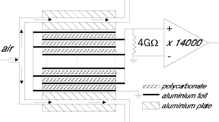
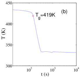
Figure 1: Polycarbonate experimental set-up(a) Design of polycarbonate capacitance cell. (b) Typical temperature quench: from $T_{i}=453\,K$ to $T_{f}=333\,K$, the origin of $t_{w}$ is set at $T=T_{g}$.

In our experiment polycarbonate is used as the dielectric of a capacitor. The capacitor is composed by $14$ cylindrical capacitors in parallel in order to reduce the resistance of the sample and to increase its capacity [20]. Each capacitor is made of two aluminum electrodes, $12\mu m$ thick, and by a disk of polycarbonate of diameter $12cm$ and thickness $125\mu m$. The experimental set-up is shown in Fig.  1(a). The $14$ capacitors are sandwiched together and put inside two thick aluminum plates which contain an air circulation used to regulate the sample temperature. This mechanical design of the capacitor is very stable and gives very reproducible results even after many temperature quenches. The capacitor is inside 4 Faraday screens to insulate it from external noise. The temperature of the sample is controlled within a few percent. Fast quenches of about $1K/s$ are obtained by injecting Nitrogen vapor in the air circulation of the aluminum plates. The electrical impedance of the capacitor is $Z(\omega,t_{w})=R/(1+i\omega\ R\ C)$, where $C$ is the capacitance and $R$ is a parallel resistance which accounts for the complex dielectric susceptibility. This is measured by a lock-in amplifier associated with an impedance adapter [20]. The noise spectrum $S_{Z}(\omega,t_{w})$ of the impedance $Z(\omega,t_{w})$ is:

$$S_{Z}(f,t_{w})=4\ k_{B}\ T_{eff}(f,t_{w})\ Re[Z(\omega,t_{w})]={4\ k_{B}\ T_{eff}(f,t_{w})\ R\over 1+(\omega\ R\ C)^{2}}$$ (1)

where $k_{B}$ is the Boltzmann constant and $T_{eff}$ is the effective temperature of the sample. This effective temperature takes into account the fact that FDT (Nyquist relation for electric noise) can be violated because the polymer is out of equilibrium during aging, and in general $T_{eff}>T$, with $T$ the temperature of the thermal bath. Of course when FDT is satisfied then $T_{eff}=T$. In order to measure $S_{Z}(f,t_{w})$, we have made a differential amplifier based on selected low noise JFET(2N6453 InterFET Corporation), whose input has been polarized by a resistance $R_{i}=4G\Omega$. Above $2Hz$, the input voltage noise of this amplifier is $5nV/\sqrt{Hz}$ and the input current noise is about $1fA/\sqrt{Hz}$. The output signal of the amplifier is directly acquired by a NI4462 card. It is easy to show that the measured spectrum at the amplifier input is:

$$S_{V}(f,t_{w}) = {4\ k_{B}\ R\ R_{i}\ \ (\ T_{eff}(f,t_{w})\ R_{i}+\ T_{R}\ R+S_{\xi}(f)\ R\ R_{i})\over(R+R_{i})^{2}+(\omega\ R\ R_{i}\ C)^{2}}+S_{\eta}(f)$$ (2)

where $T_{R}$ is the temperature of $R_{i}$ and $S_{\eta}$ and $S_{\xi}$ are respectively the voltage and the current noise spectrum of the amplifier. In order to reach the desired statistical accuracy of $S_{V}(f,t_{w})$, we averaged the results of many experiments. In each of these experiments the sample is first heated to $T_{i}=1.08T_{g}$. It is maintained at this temperature for several hours in order to reinitialize its thermal history. Then it is quenched from $T_{i}$ to the working final temperature $T_{f}$ where the aging properties are studied. The maximum quenching rate from $T_{i}$ to $T_{f}$ is $1K/s$. A typical thermal history of a fast quench is shown in Fig. 1(b). The reproducibility of the capacitor impedance, during this thermal cycle is always better than $1\%$. The origin of aging time $t_{w}$ is the instant when the capacitor temperature is at $T_{g}\simeq 419K$, which of course may depend on the cooling rate. However adjustment of $T_{g}$ of a few degrees will shift the time axis by at most $30s$, without affecting our results.

2.2 Response and noise measurements

Before discussing the time evolution of the dielectric properties and of the thermal noise at $T_{f}$ we show in Fig. 2 the dependence of $R$ and $C$ measured at $1Hz$ as a function of temperature, which is ramped as a function of time as indicated in the inset of Fig. 2(a). We notice a strong hysteresis between cooling and heating. In the figure $T_{\alpha}$ is the temperature of the $\alpha$ relaxation at $1Hz$. The other circles on the curve indicate the $T_{f}$ where the aging has been studied. We have performed measurements at $T_{f}=0.79T_{g},0.93T_{g},0.98T_{g}$ using fast and slow quenches. The cooling rate is $1K/s$ and $0.06K/s$ for the fast and slow quenches respectively. As at $T_{f}=0.98T_{g}$ the dielectric constant strongly depends on temperature (see Fig.2), the temperature stability has to be much better at $T_{f}=0.98T_{g}$ than at the two other smaller $T_{f}$. Because of this good temperature stability needed at $T_{f}=0.98T_{g}$ it is impossible to reach this temperature too fast. Therefore at 0.98 $T_{g}$ we have performed only measurements after a slow quench.

          (a)                                                      (b)

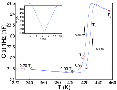
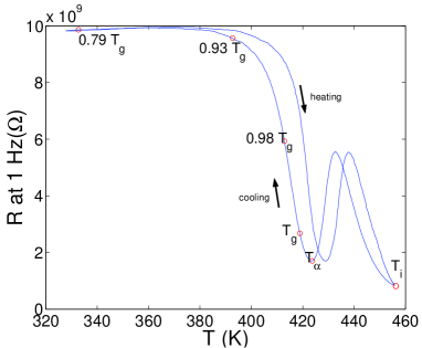
Figure 2: Polycarbonate response function at 1Hz(a) Dependence of $C$, measured at $1Hz$, on temperature, when $T$ is changed as function of time as indicated in the inset. (b) Dependence of $R$, measured at $1Hz$, on $T$. $T_{\alpha}$ is the temperature of the $\alpha$ relaxation at$1Hz$, $T_{g}$ is the glass transition temperature. The other circles on the curve indicate the $T_{f}$ where aging has been studied.

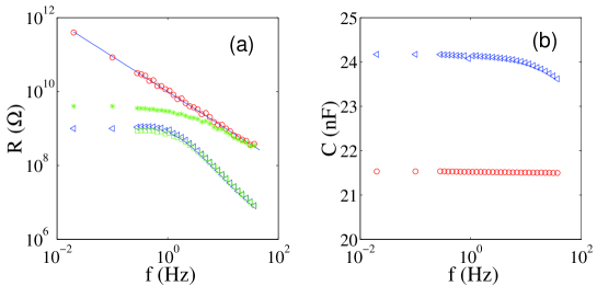
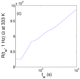
Figure 3: Polycarbonate response function(a) Polycarbonate resistance $R$ as a function of frequency measured at $T_{i}=1.08T_{g}$ ($\vartriangleleft$) and at $T_{f}=0.79T_{g}$ ($\circ$)(after a fast quench). The effect of the $4G\Omega$ input resistance in parallel with the polycarbonate impedance is also shown at $T=433K$ ($\square$) and at $T=333K$ ($\ast$). (b) Polycarbonate capacitance versus frequency measured at $T_{i}=433K$ ($\vartriangleleft$) and at $T_{f}=333K$ ($\circ$). (c) Typical aging of $R$ measured at $1Hz$ as a function of $t_{w}$

We first describe the results after a fast quench at the smallest temperature, that is $T_{f}=0.79T_{g}$. In Fig. 3(a) and (b), we plot the measured values of $R$ and $C$ as a function of $f$ at $T_{i}=1.08T_{g}$ and at $T_{f}$ for $t_{w}\geqslant 200s$. The dependence of $R$, at $1Hz$, as a function of time is shown in Fig. 3(c). We see that the time evolution of $R$ is logarithmic in time for $t>300s$ and that the aging is not very large at $T_{f}=0.79T_{g}$, it is only $10\%$ in 3 hours. At higher temperature close to $T_{g}$ aging is much larger.

Looking at Fig. 3(a) and (b), we see that lowering temperature $R$ increases and $C$ decreases. As at $0.79T_{g}$ aging is small and extremely slow for $t_{w}>200s$ the impedance can be considered constant without affecting our results. From the data plotted in Fig. 3 (a) and (b) one finds that $R=10^{10}(1\pm 0.05)\ f^{-1.05\pm 0.01}\ \Omega$ and $C=(21.5\pm 0.05)nF$. In Fig. 3(a) we also plot the total resistance at the amplifier input which is the parallel of the capacitor impedance with $R_{i}$. We see that at $T_{f}$ the input impedance of the amplifier is negligible for $f>10Hz$, whereas it has to be taken into account at slower frequencies.

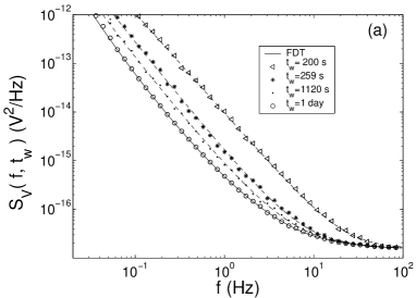
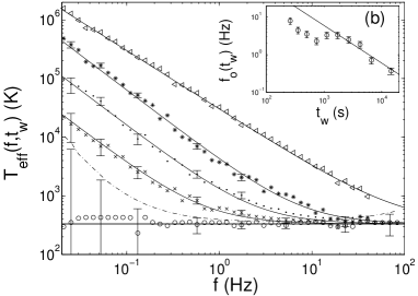
Figure 4: Voltage noise and effective temperature in polycarbonate after a fast quench(a) Noise power spectral density $S_{V}(f,t_{w})$ measured at $T_{f}=333K$ and different $t_{w}$. The spectra are the average over seven quenches. The continuous line is the FDT prediction. Dashed lines are the fit obtained using eq.2 and eq.3 (see text for details). (b) Effective temperature vs frequency at $T_{f}=333K$ for different aging times: $(\vartriangleleft)\ tw=200\ s$, $(\ast)\ tw=260s$, $\bullet\ tw=2580s$, $(\times)t_{w}=6542s$, $(\circ)t_{w}=1\ day$. The continuous lines are the fits obtained using eq.3. The horizontal straight line is the FDT prediction. The dot dashed line corresponds to the limit where the FDT violation can be detected. In the inset the frequency $f_{o}(t_{w})$, defined in eq.3,is plotted as a function of $t_{w}$. The continuous line is not a fit, but it corresponds to $f_{o}(t_{w})\propto 1/t_{w}$.

Fig. 4(a) represents the evolution of $S_{V}(f,t_{w})$ after the fast quench. Each spectrum is obtained as an average in a time window starting at $t_{w}$. The time window increases with $t_{w}$ so to reduce error for large $t_{w}$. The results of 7 quenches have been averaged. At the longest time ($t_{w}=1\ day$) the equilibrium FDT prediction (continuous line) is quite well satisfied. We clearly see that FDT is strongly violated for all frequencies at short times. Then high frequencies relax on the FDT, but there is a persistence of the violation for lower frequencies. The amount of the violation can be estimated by the best fit of $T_{eff}(f,t_{w})$ in eq.2 where all other parameters are known. We started at very large $t_{w}$ when the system is relaxed and $T_{eff}=T$ for all frequencies. Inserting the values in eq.2 and using the $S_{V}$ measured at $t_{w}=1day$ we find $T_{eff}\simeq 333K$, within error bars for all frequencies (see Fig. 4b). At short $t_{w}$ data show that $T_{eff}(f,t_{w})\simeq T_{f}$ for $f$ larger than a cutoff frequency $f_{o}(t_{w})$ which is a function of $t_{w}$. In contrast, for $f<f_{o}(t_{w})\ \$ we find that $T_{eff}$ is: $T_{eff}(f,t_{w})\propto f^{-A(t_{w})}$, with $A(t_{w})\simeq 1$. This frequency dependence of $T_{eff}(f,t_{w})$ is quite well approximated by

$$T_{eff}(f,t_{w})=T_{f}\ [\ 1\ +\ ({f\over f_{o}(t_{w})})^{-A(t_{w})}\ ]$$ (3)

where $A(t_{w})$ and $f_{o}(t_{w})$ are the fitting parameters. We find that $1<A(t_{w})<1.2$ for all the data set. Furthermore for $t_{w}\geq 250$, it is enough to keep $A(t_{w})=1.2$ to fit the data within error bars. For $t_{w}<250s$ we fixed $A(t_{w})=1$. Thus the only free parameter in eq.3 is $f_{o}(t_{w})$. The continuous lines in Fig. 4(a) are the best fits of $S_{V}$ found inserting eq.3 in eq.2.

In Fig. 4(b) we plot the estimated $T_{eff}(f,t_{w})$ as a function of frequency at different $t_{w}$. We see that just after the quench $T_{eff}(f,t_{w})$ is much larger than $T_{f}$ in all the frequency interval. High frequencies rapidly decay towards the FDT prediction whereas at the smallest frequencies $T_{eff}\simeq 10^{5}K$. Moreover we notice that low frequencies decay more slowly than high frequencies and that the evolution of $T_{eff}(f,t_{w})$ towards the equilibrium value is very slow. From the data of Fig. 4(b) and eq.3, it is easy to see that $T_{eff}(f,t_{w})$ can be superposed onto a master curve by plotting them as a function of $f/f_{o}(t_{w})$. The function $f_{o}(t_{w})$ is a decreasing function of $t_{w}$, but the dependence is not a simple one, as it can be seen in the inset of Fig. 4(b). The continuous straight line is not fit, it represents $f_{o}(t_{w})\propto 1/t_{w}$ which seems a reasonable approximation for these data for $t>1000s$. For $t_{w}>10^{4}s$ we find the $f_{o}<1Hz$. Thus we cannot follow the evolution of $T_{eff}$ anymore because the contribution of the experimental noise on $S_{V}$ is too big, as it is shown in Fig. 4(b) by the increasing of the error bars for $t_{w}=1\ day$ and $f<0.1Hz$.

We do not show the same data analysis for the other working temperature after a fast quench, because the same scenario appears in the range $0.79T_{g}<T<0.93T_{g}$, where the low frequency dielectric properties are almost temperature independent (see Fig. 2(b)). The only important difference to mention here is that aging becomes faster and more pronounced as the temperature increases. At $T_{f}=0.93T_{g}$, the losses of the capacitor change of about $50\%$ in about $3h$, but all the spectral analysis performed after a fast quench gives the same evolution. We can just notice that $T_{eff}$ for $T=0.93T_{g}$ is higher than that at $T=0.79T_{g}$. At $T=0.93T_{g}$, $T_{eff}$ is well fitted by eq.3. It is enough to keep $A(t_{w})=1$ for all $t_{w}$ and $f_{o}(t_{w})\sim 1/t_{w}^{1.5}$, see fig.5a). We notice that at $0.93T_{g}$ the power law behaviour is well established, whereas it was more doubtful at $0.73T_{g}$. The dependence of $T_{eff}$ as a function of $t_{w}$ is plotted in fig.5 for two values of $f$ and has also a power law dependence on $t_{w}$.

          (a)                                                      (b)

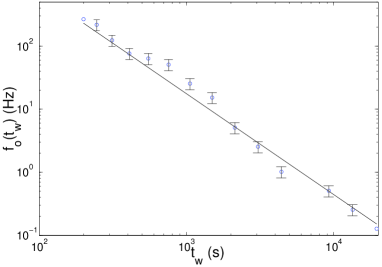
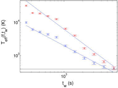
Figure 5: $f_{o}$ and $T_{eff}$ as a function of $t_{w}$ at $T_{f}=0.93T_{g}$ after a fast quench. (a) $f_{o}$ defined in eq.3 as a function of $t_{w}$ (b) Evolution of $T_{eff}$ at two different frequencies $(\circ)\ 7Hz$ and $(\triangleleft)\ 2Hz$

For $T>0.93T_{g}$ fast quenches cannot be performed for the technical reasons mentioned at the beginning of section 3). The results are indeed quite different. Thus we will not consider, for the moment, the measurement at $T_{f}=0.98T_{g}$ and we will mainly focus on the measurements done in the range $0.79T_{g}<T<0.93T_{g}$ with fast quenches. For these measurements the spectral analysis on the noise signal indicates that Nyquist relation (FDT) is strongly violated for a long time after the quench. The question is now to understand the reasons of this violation.

2.3 Statistical analysis of the noise

In order to understand the origin of such large deviations in our experiment we have analyzed the noise signal. We find that the signal is characterized by large intermittent events which produce low frequency spectra proportional to $f^{-\alpha}$ with $\alpha\simeq 2$. Two typical signals recorded at $T_{f}=0.79T_{g}$ for $1500\,s<t_{w}<1900\,s$ and $t_{w}>75000\,s$ are plotted in Fig. 6. We clearly see that in the signal recorded for $1500\,s<t_{w}<1900\,s$ there are very large bursts which are on the origin of the frequency spectra discussed in the previous section. In contrast in the signal which was recorded at $t_{w}>75000\,s$, when FDT is not violated, the bursts totally disappear (Fig. 6b).

          (a)                                                                       (b)

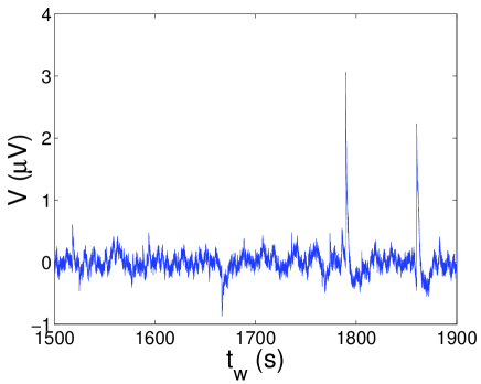
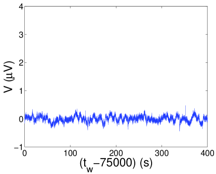
Figure 6: Voltage noise signal in polycarbonate after a fast quench Typical noise signal of polycarbonate measured at $T_{f}=333K$ for $1500s<t_{w}<1900s$ (a) and $t_{w}>75000s$ (b)

The probability density function (PDF) of these signals is shown in Fig. 7 (a). We clearly see that the PDF, measured at small $t_{w}$, has very high tails which becomes smaller and smaller at large $t_{w}$. Finally the Gaussian profile is recovered after $24h$. The PDF are very symmetric in their gaussian parts, i.e. 3 standard deviations. The tails of the PDF are exponential and are decreasing functions of $t_{w}$.

          (a)                                                                       (b)

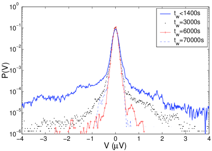
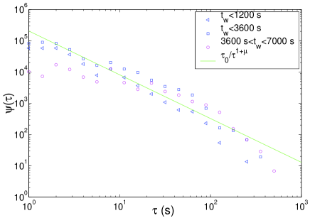
Figure 7: PDF of voltage noise in polycarbonate after a fast quench at $T_{f}=0.79T_{g}$. (a) The large tails of the PDF at early $t_{w}$ are a signature of strong intermittency. (b) Histogram of time interval $\tau$ between two successive pulses: $\Psi(\tau,t_{w})$. At early $t_{w}$, $\Psi(\tau,t_{w})$ is power law distributed.

The time interval $\tau$ between two successive pulses is power law distributed. In order to study this distribution $\Psi(\tau,t_{w})$ of $\tau$, we have first selected the signal fluctations with amplitude larger than a fixed threshold, which has been chosen between 3 and 4 standard deviations of the equilibrium noise, i.e. the noise predicted by the FDT. We have then measured the time intervals $\tau$ between two successive large fluctuations. The histogram $\Psi(\tau,t_{w})$ computed for $t_{w}<20min$ and for $20min<t_{w}<3h$ is plotted in Fig. 7(b). We clearly see that $\Psi(\tau,t_{w})$ is a power law, specifically $\Psi(\tau)\propto\frac{1}{\tau^{1+\mu}}$ with $\mu\simeq 0.4\pm 0.1$. This result agree with one of the hypothesis of the trap model[31]-[32], which presents non-trivial violation of FDT associated to an intermittent dynamics. In the trap model $\tau$ is a power-law-distributed quantity with an exponent 1+$\mu$ that, in the glass phase, is smaller than 2. However, there are important differences between the dynamics of our system and that of the trap model. Indeed in this model one finds short and large $\tau$ for any $t_{w}$ which is in contrast with our system because the probability of finding short $\tau$ seems to decrease as a function of $t_{w}$. But this effect could be a consequence of the imposed threshold. It seems that there is no correlation between the $\tau$ and the amplitude of the associated bursts. Finally, the maximum distance $\tau_{max}$ between two successive pulses grows as a function of $t_{w}$ logarithmically, that is $\tau_{max}=[10+152log(t_{w}/300)]s$ for $t_{w}>300s$. This slow relaxation of the number of events per unit of time shows that the intermittency is related to aging.

The same behaviour is observed at $T_{f}=0.93T_{g}$ after a fast quench. The PDF of the signals measured at $T_{f}=0.93T_{g}$ are shown in Fig. 8(a). The behaviour is the same except for the relaxation rate towards the Gaussian distribution which is faster in this case, because the aging effects are larger at this temperature. From these measurements one concludes that after a fast quench the electrical thermal noise is strongly intermittent and non-Gaussian. The number of intermittent events increases with the temperature : for $T_{f}=0.93T_{g}$, $T_{eff}$ is higher than for $T_{f}=0.79T_{g}$ and PDF tails are more important.

          (a)                                                                       (b)

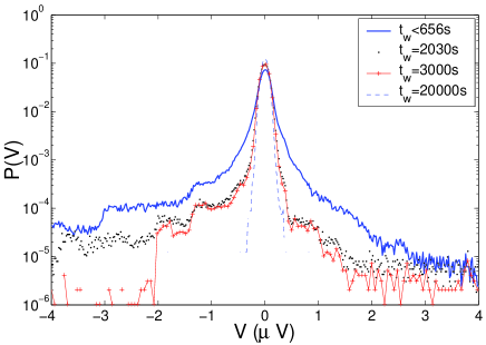
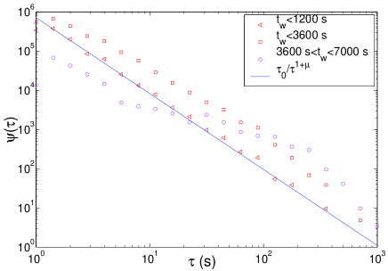
Figure 8: PDF of voltage noise in polycarbonate after a fast quench at $0.93T_{g}$(a) PDF of the noise signal of polycarbonate measured at various $t_{w}$. (b) Histograms $\Psi(\tau,t_{w})$, following at early $t_{w}$ a $1/\tau^{1+\mu}$ law with $\mu=0.9\pm 0.1$.

The histograms $\Psi(\tau,t_{w})$ are shown Fig. 8 (b). The behaviour is the same with $\mu=0.9\pm 0.1$. By comparing $\Psi(\tau,t_{w})$ for short $\tau$ and short $t_{w}$ there are more events at $0.93T_{g}$ (Fig. 8 (b)) than at $0.79T_{g}$ (Fig. 7 (b)). This is consistent with activation processes for the aging dynamics. Indeed the probability of jumping from a potential well to another increases with temperature. Thus one expects to find more events at high temperature than at low temperature.

2.4 Influence of the quench speed.

The intermittent behaviour described in the previous sections depends on the quench speed. In Fig. 9(a) we plot the PDF of the signals measured after a slow quench ($3.6\,K/min$) at $T_{f}=0.93T_{g}$. We clearly see that the PDF are very different: intermittency has almost disappeared. The comparison between the fast quench and the slow quench merits a special comment. During the fast quench $T_{f}=0.93T_{g}$ is reached in about $100\,s$ after the passage of $T$ at $T_{g}$. For the slow quench this time is about $1000\,s$. Therefore one may wonder whether after $1000s$ of the fast quench one recovers the same dynamics of the slow quench. By comparing the PDF of Fig. 8(a) with those of Fig. 9(a) we clearly see that this is not the case. Furthermore, by comparing the histograms of Fig. 8(b) with those of Fig.9(b), we clearly see that there are less events separated by short $\tau$ for the slow quench. Therefore one deduces that the polymer is actually following a completely different dynamics after a fast or a slow quench [33, 34]. This is a very important observation that can be related to well known effects of response function aging. The famous Kovacs effect is an example[4] where depending on the cooling rate the isothermal compressibility presents a completely different time evolution.

          (a)                                                                       (b)

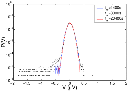
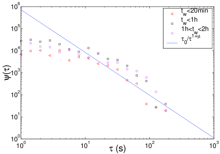
Figure 9: PDF of voltage noise in polycarbonate after a slow quench at $T_{f}=0.93T_{g}$. (a) No intermittency is visible after a slow quench at $3.6K/min$. (b) Histograms $\Psi(\tau,t_{w})$ after a slow quench. The line corresponds to the $\tau_{0}/\tau^{1+\mu}$ fit of Fig. 8(b), where $\mu=0.93$.

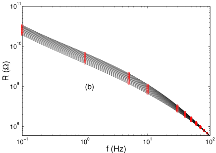
Figure 10: Capacitance losses at $T_{f}=0.98T_{g}$ after a slow quench. Resistance as a function of frequency for different $t_{w}$ from $t=100s$ (lower curve) to $t_{w}=14400s$.

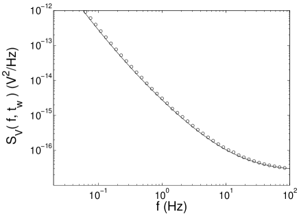
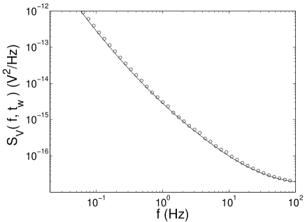
Figure 11: Power spectral density of the capacitance noise at $T_{f}=0.98T_{g}$ after a slow quench. $S_{V}(f,t_{w})$ as a function of $f$ for two different time: (a) $t_{w}=200s$, (b) $t_{w}=7200s$. Circles stand for measurement points, whereas the continuous line is the FDT prediction.

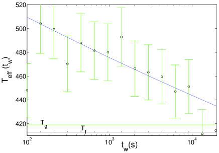
Figure 12: $T_{eff}$ as a function of time at $T_{f}=0.98T_{g}$ after a slow quench. $T_{eff}$ averaged in the frequency band $[1Hz-10Hz]$. It has been computed from the spectra $S_{V}(f,t_{w})$ and the measured $(R,C)$ using eq.2

.

          (a)                                                                       (b)

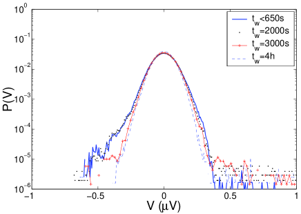
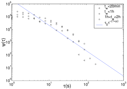
Figure 13: PDF of the signal at $T_{f}=0.98T_{g}$ after a slow quench. (a) PDF of the signal. No intermittency is visible. (b) Histograms $\Psi(\tau,t_{w})$ after a slow quench. The continuous line represent the $1/\tau^{1+\mu}$ law where we chose $\mu=T_{f}/T_{g}$ to compare with the theoretical estimation of the trap model.

2.5 $T_{eff}$ after a slow quench

In the previous section we have shown that the intermittent aging dynamics is strongly influenced by the cooling rate. We discuss in this section the behaviour of the effective temperature after a slow quench. We use for this purpose the measurement at $T_{f}=0.98T_{g}$. The time evolution of the response function is much larger at this temperature than at $T_{f}=0.79T_{g}$ as it can be seen in fig.10. It is about $50\%$ at the small frequencies, therefore it has to be kept into account in the evaluation of FDT. The spectrum of the capacitance noise measured at $0.98T_{g}$ is plotted for two different times in fig.11. The continuous lines represents the FDT predictions computed using the measured response function reported in fig.10. We clearly see that the experimental points are very close to the FDT predictions, thus the violation of FDT, if it exists, is very small. To check this point, we have computed $T_{eff}$ in the range $[1Hz-10Hz]$, which is plotted as a function of time in fig.12. Although the error bars are rather large, we clearly see that $T_{eff}$ decreases logarithmically as a function of time. We also notice that the maximum violation at short times is about $25\%$ which is much smaller than that measured at smaller $T_{f}$ after a fast quench. The PDF of the noise signal at $0.98T_{g}$ are plotted in fig.13(a) and they do not show very large tails as in the case of the intermittent dynamics. The statistics of the time intervals $\tau$ between two large events does not present any power law either (see fig.13(b)). Thus the signal statistics look much more similar to those measured at $0.93T_{g}$ after a slow quench than to the intermittent ones. This comparison shows that independently of the final temperature the intermittent behaviour is induced by the fast quench and that the FDT violation is cooling rate dependent.

3 Mechanical measurements on a Polycarbonate cantilever

In the previous section we have studied the properties of dielectrical thermal noise during the aging of polycarbonate. In this section we want to check if the thermal noise features are independent of the observable. As a second observable, we have chosen to measure the thermally excited vibrations of a cantilever made of polycarbonate.

3.1 FDT in a mechanical oscillator

The physical object of our interest is a small plate with one end clamped and the other free, i.e. a cantilever. The plate is of length $l$, width $a$, thickness $b$, mass $m_{\mathrm{Polyc}}$. On the free end of the cantilever a small golden mirror of mass $m_{\mathrm{mirror}}$ is glued. As described in the next section, this mirror is used to detect the amplitude $x_{c}$ of the transverse vibrations of the cantilever free end. The motion of the cantilever free end can be assimilated to that of a driven harmonic oscillator, which is damped only by the viscoelasticity of the polymer. Consequently, the equation of motion of the cantilever free end takes a simple form in Fourier space:

$$[-m\omega^{2}+K(\omega)]\hat{x}_{c}=\hat{F}_{\mathrm{ext}}$$ (4)

where $\hat{x}_{c}$ is the Fourier transform of $x_{c}$, $m$ is the total effective mass of the plate plus the mirror, $K=K^{\prime}+iK^{\prime\prime}$ is the complex elastic stiffness of the plate free end, and $\hat{F}_{\mathrm{ext}}$ is the Fourier transform of the external driving force. The complex $K(\omega)$ takes into account the viscoelastic nature of the cantilever. From the theory of elasticity [35] one obtains that, for low frequencies, an excellent approximations for $m$ and $K$ are:

$$m = \frac{3}{(3.52)^{2}}\,m_{\mathrm{Polyc}}+m_{\mathrm{mirror}},$$ (5)

$$\textrm{and }K = {Eab^{3}\over 4l^{3}},$$ (6)

where $E=E^{\prime}+iE^{\prime\prime}$ is the plate Young modulus. Notice that if $m_{\mathrm{mirror}}=0$, then one recovers the smallest resonant frequency of the cantilever [35]. For Polycarbonate at room temperature, $E$ is such that $E^{\prime}=2.2\times 10^{9}\textrm{ Pa}$ and $E^{\prime\prime}=2\times 10^{7}\textrm{ Pa}$, and its frequency dependence may be neglected in the range of frequency of our interest, that is from 0.1 to 100 Hz [36]. Thus we neglect the frequency dependence of $K$ in this specific example.

When $F_{\mathrm{ext}}=0$, the amplitude of the thermal vibrations of the cantilever free end $x_{T}$ is linked to its response function $\chi$ via the FDT [37]:

$$\langle|{\hat{x}_{T}|}^{2}\rangle=\frac{2k_{B}T}{\omega}\,\mathrm{Im}\,\hat{\chi},$$ (7)

where $\langle{|\hat{x}_{T}|}^{2}\rangle$ is the thermal fluctuations spectral density of $x_{c}$, $k_{B}$ the Boltzmann constant and $T$ the temperature. From Eq. 4 one obtains that the response function of the harmonic oscillator is

$$\hat{\chi}=\frac{\hat{x}_{c}}{\hat{F}_{\mathrm{ext}}}={1\over m[{\omega_{0}}^{2}-\omega^{2}-i\,(\mathrm{sign}\,\omega)\,\gamma{\omega_{0}}^{2}]},$$ (8)

where ${\omega_{0}}^{2}=K^{\prime}/m$ and $\gamma=K^{\prime\prime}/K^{\prime}$.

Inserting Eq. 8 into Eq. 7, one can compute the thermal fluctuations spectral density of the Polycarbonate cantilever for positive frequencies:

$$\langle{|\hat{x}_{T}|}^{2}\rangle=\frac{2k_{B}T}{\omega}\frac{\gamma{\omega_{0}}^{2}}{m[({\omega_{0}}^{2}-{\omega}^{2})^{2}+(\gamma{\omega_{0}}^{2})^{2}]}.$$ (9)

Notice that $\langle{|{\hat{x}_{T}}|}^{2}\rangle\sim\omega^{-1}$ for $\omega\ll\omega_{0}$, because the viscoelastic damping $K^{\prime\prime}$ is constant in our frequency range. In the case of a viscous damping (for example, a cantilever immersed in a viscous fluid) $K^{\prime\prime}=\alpha\,\omega$, where $\alpha$ is proportional to the fluid viscosity and to a geometry dependent factor. Then the thermal fluctuations spectral density of the cantilever free end, in the case of viscous damping, is

$$\langle{|\hat{x}_{T}|}^{2}\rangle=\frac{2k_{B}T\,\alpha}{m^{2}[(\omega_{0}^{2}-\omega^{2})^{2}+(\frac{\alpha}{m}\omega)^{2}]},$$ (10)

which is constant for $\omega\ll\omega_{0}$. Therefore, the thermal fluctuations spectral density shape depends on $K^{\prime\prime}(\omega)$. In the case of a viscoelastic damping (Eq. 9), the thermal noise increases when $\omega$ goes to 0, and with a suitable choice of the parameters the low frequency spectral density of an aging polymer can be measured using this method.

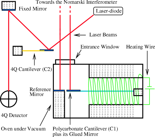
Figure 14: Experimental setup for measuring the mechanical noise in polycarbonate The polycarbonate cantilever (C1) is inside an oven to control the temperature. Its displacement is measured by a very sensitive Nomarski Interferometer. The cantilever (C2) the laser diode, and the 4Q detector, are use for the noise reduction technique (see text).

However, the cantilever is also sensitive to the mechanical noise, and the total displacement $x_{c}$ of the cantilever free end actually reads $x_{c}=x_{T}+x_{\mathrm{acc}}$, where $x_{\mathrm{acc}}$ is the displacement induced by the external mechanical noise. Thus, it is important to compute the signal-to-noise ratio (SNR) of our apparatus, which we define as the ratio between the thermal fluctuations and the mechanical noise spectral densities. All the details on the optimization of the SNR can be found in ref.[38].

3.2 Experimental apparatus

Let us estimate the amplitude of $\sqrt{{\langle{|{\hat{x}_{T}}|}^{2}\rangle}}$ at $\nu=\omega/2\pi=1\textrm{ Hz}$ for the following choice of the parameters: $\gamma\simeq 10^{-2}$, $l\simeq 10\textrm{ mm}$, $a\simeq 1\textrm{ mm}$, $b=125\ \mu\mathrm{m}$ and $m_{\mathrm{mirror}}\lesssim 10^{-3}\textrm{ g}$. We find $\nu_{0}\simeq 100\textrm{ Hz}$ and $\sqrt{{\langle{|{\hat{x}_{T}(1\textrm{ Hz})}|}^{2}\rangle}}\simeq 10^{-11}\textrm{ m}/\sqrt{\mathrm{Hz}}$, which is a very small signal. As a consequence, extremely small vibrations of the environment may greatly perturb the measurement. Therefore, to increase the signal-to-noise ratio of the measurement, one has to reduce the coupling of the cantilever to the environmental noise (acoustic and seismic) using vibration isolation systems. This may be not enough in this specific case because of the smallness of the thermal fluctuations. Therefore we have applied an original noise subtraction technique described in ref.[38] in order to recover $x_{T}$ from the measurement of $x_{c}$.

The measurement of $x_{c}$ is done using a Nomarski interferometer (for detailed reviews, see [39, 40, 41]) which uses the mirror glued on the Polycarbonate cantilever in one of the two optical paths. The interferometer noise is about $5\times 10^{-14}\textrm{ m}/\sqrt{\mathrm{Hz}}$, which is two orders of magnitude smaller than the cantilever thermal fluctuations. The cantilever is inside an oven under vacuum. A window allows the laser beam to go inside (cf Fig. 14). The size of the Polycarbonate cantilever are, $l\simeq 13.5\textrm{ mm}$, $a\simeq 1\textrm{mm}$ and $b=125\ \mu\mathrm{m}$, and the mirror mass is $m_{\mathrm{mirror}}\lesssim 10^{-3}\textrm{ g}$ such that $\nu_{0}\simeq 100\textrm{ Hz}$. As already mentioned, the cantilever is sensitive to unavoidable mechanical vibrations which are the main source of error and strongly reduce the signal to noise ratio. To improve the signal-to-noise ratio we have applied the reduction technique described in ref.[38]. This technique is based on a mechanical noise detection system whose scheme is shown in fig.14 : A second cantilever, the parameter of which are tuned to be only sensitive to external vibration (and not to its own thermal fluctuations), is used to subtract the mechanical noise component from the signal of the polycarbonate cantilever. More details can be found in ref.[38].

          (a)                                                                       (b)

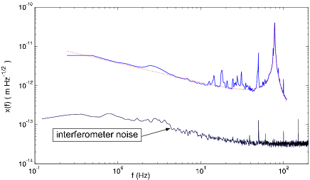
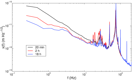
Figure 15: Spectra of the thermal noise of the polycarbonate cantilever (a) Equilibrium spectrum at 293K of the cantilever tip thermal fluctuations. The dashed line is the FDT prediction. the noise of the detection system (spectrum in the bottom of the figure) is shown for comparison. (b) Time evolution of the cantilever noise spectrum recorded at three different times $tw=20min,\ 2h,\ 18h$ after that the temperature $T_{f}=393K$ has been reached from below (see text)

3.3 Experimental results

We first check whether the polycarbonate cantilever verifies the FDT at room temperature. The results are shown in fig.15a), where the square root of the spectral density is plotted as a function of f. The dashed line is the FDT prediction obtained from a direct measurement of the cantilever response function. The agreement is good. For comparison the square root of the spectral density of the interferometer noise is plotted too. We see that the SNR is quite good. The extra picks on the spectrum of $x_{c}$ come from residual mechanical vibrations. This figure shows that the experimental system is well suited to study fluctuation relations in an aging material. To study the polycarbonate cantilever noise after a quench we used a protocol that is different from that described in section 1) for dielectric measurement. As polycarbonate is almost liquid above $T_{g}$ it is impossible to keep it in the above described measurement cell. Thus we put the cantilever inside a box which has in the bottom a groove where the cantilever fits perfectly inside. Then this box is first heated at $T_{i}=460K$ and then rapidly cooled by putting it into a cool water. Thus in a few seconds the cantilever is quenched from $460K$ to about $280K$. Then the cantilever is installed inside the measurement cell that is heated to the working temperature $T_{f}$ which is now reached from low temperature. The polycarbonate ages anyway: it is well known that in aging systems the time spent at low temperature does not affect the aging at high temperature. We report here a measurement of the time evolution of the noise spectrum performed at $T_{f}=0.93T_{g}$. A typical evolution of the polycarbonate cantilever fluctuation spectrum is plotted in fig.15. The spectra recorded at $t_{w}=20min,\ 2h,\ 18h$ are shown. We see that at very short time the spectrum present a very large power law behaviour at low frequencies. This component relaxes towards equilibrium in several hours. As the response function of the cantilever evolves of just a few percent during the same amount of time it is clear that the violation of FDT is very large also in the case of this mechanical measurement. The reason is the presence of a strong intermittency as in the case of the dielectric measurements described in Sec. 2.

4 Thermal noise in a colloidal glass

We review in this section results on electrical noise measurements in Laponite during the transition from a fluid like solution to a solid like colloidal glass. The main control parameter of this transition is the concentration of Laponite[42], which is a synthetic clay consisting of discoid charged particles. It disperses rapidly in water to give gels even for very low mass fraction. Physical properties of this preparation evolves for a long time, even after the sol-gel transition, and have shown many similarities with standard glass aging[3]. Recent experiments have even proved that the structure function of Laponite at low concentration (less than $3\%$ mass fraction) is close to that of a glass, suggesting the colloidal glass appellation [43].

In previous studies, we showed that the early stage of this transition was associated with a small aging of its bulk electrical conductivity, in contrast with a large variation in the noise spectrum at low frequency. As a consequence, the FDT in this material appeared to be strongly violated at low frequency in young samples, and it is only fulfilled for high frequencies and long times[14, 15, 18, 19]. As in polycarbonate, this effect was shown to arise from a strong intermittency in the electrical noise of the samples, characterized by a strong deviation to a standard gaussian noise[19]. We summarize these results in the first part of this section, before presenting preliminary results on the role of concentration in the noise behavior.

4.1 Experimental setup

The experimental setup is similar to that of previous experiments[14, 15, 19]. The Laponite[42] dispersion is used as a conductive material between the two golden coated electrodes of a cell. It is prepared in a clean $\mathrm{N_{2}}$ atmosphere to avoid $\mathrm{CO_{2}}$ and $\mathrm{O_{2}}$ contamination, which perturbs the aging of the preparation and the electrical measurements. Laponite particles are dispersed at a concentration of $2.5\%$ to $3\%$ mass fraction in pure water under vigorous stirring for $300\,s$. To avoid the existence of any initial structure in the sol, we pass the solution through a $1\,\mu m$ filter when filling the cell. This instant defines the origin of the aging time $t_{w}$ (the filling of the cell takes roughly two minutes, which can be considered the maximum inaccuracy of $t_{w}$). The sample is then sealed so that no pollution or evaporation of the solvent can occur. At these concentrations, light scattering experiments show that Laponite[42] structure functions are still evolving several hundreds hours after the preparation, and that solid like structures are only visible after $100\,h$[3]. We only study the beginning of this glass formation process.

The two electrodes of the cell are connected to our measurement system, which records either the impedance value or the voltage noise across it. The electrical impedance of the sample is the sum of two effects: the bulk is purely conductive, the ions of the solution following the forcing field, whereas the interfaces between the solution and the electrodes give mainly a capacitive effect due to the presence of the Debye layers[44]. This behavior has been validated using a four-electrode potentiostatic technique[45] to make sure that the capacitive effect is only due to the surface. In order to probe mainly bulk properties, the geometry of the cell is tuned to push the surface contribution to low frequencies: the cell consists in two large reservoirs where the fluid is in contact with the electrodes (area of $25\,cm^{2}$), connected through a small rigid tube — see Fig. 16(b). The main contribution to the electrical resistance of the cell is given by the Laponite sol contained in this tube connecting the two tanks. Thus by changing the length and the section of this tube the total bulk resistance of the sample can be tuned around $R_{opt}=100\,k\Omega$, which optimizes the signal to noise ratio of voltage fluctuations measurements with our amplifier. The cut-off frequency of the equivalent R-C circuit (composed by the series of the Debye layers plus the bulk resistance) is about $20\,mHz$. In other words above this frequency the imaginary part of the cell impedance is about zero, as shown in Fig. 16(a). The time evolution of the resistance of one of our sample is plotted in Fig. 16(c): it is still decaying in a non trivial way after $24h$, showing that the sample has not reached any equilibrium yet. This aging is consistent with that observed in light scattering experiments[3].

(a)                                          (b)                                                (c)

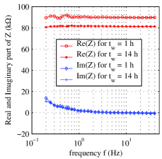
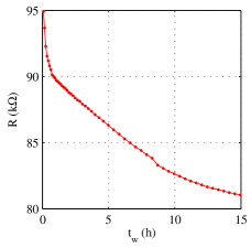
Figure 16: Impedance of a $2.5\,wt\%$ Laponite cell. (a) Frequency dependance of a sample impedance for 2 different aging times ($t_{w}=1\,h$ and $t_{w}=14\,h$). (b) Cell design and equivalent electrical model (c) Time evolution of the bulk resistance: this long time evolution is the signature of the aging of the colloidal suspension. In spite of the decreasing mobility of Laponite particles in solution during the formation of the gel, the electrical conductivity increases.

4.2 Electric noise measurements in Laponite

In order to study the voltage fluctuations across the Laponite cell, we use a custom ultra low noise amplifier to raise the signal level before acquisition. To bypass any offset problems during this strong amplification process, passive high pass filtering above $30\,mHz$ is applied. The power spectrum density of the voltage noise of a $2.5\,wt\%$ Laponite preparation is shown in Fig. 17. As the dissipative part of the impedance $Re(Z)$ is weakly time and frequency dependent, one would expect from the Nyquist formula[46] that so does the voltage noise density $S_{Z}$. But as shown in Fig. 17, we have a large deviation from this prediction for the lowest frequencies and earliest times of our experiment: $S_{Z}$ changes by several orders of magnitude between highest values and the high frequency tail. For long times and high frequencies, the FDT holds and the voltage noise density is that predicted from the Nyquist formula for a pure resistance at room temperature ($300\,K$). In order to be sure that the observed excess noise is not due to an artifact of the experimental procedure, we filled the cell with an electrolyte solution with a pH close to that of the Laponite preparation such that the electrical impedance of the cell was the same (specifically: $NaOH$ solution in water at a concentration of $10^{-3}\,mol\cdot l^{-1}$). In this case, the noise spectrum was flat and in perfect agreement with the Nyquist formula[14].

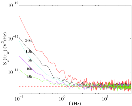
Figure 17: Voltage noise density for a $2.5\,wt\%$ Laponite sample. The power spectrum density of voltage fluctuations across the impedance of a $2.5\,wt\%$ Laponite cell exhibit strong aging, and match the Nyquist formula prediction (horizontal dashed line) only for long times or large frequencies.

Aiming at a better understanding of the physics underlaying such a behavior, we have directly analyzed the voltage noise across the Laponite cell. This test can be safely done in our experimental configuration as the amplifier noise is negligible with respect to the voltage fluctuations across cell, even for the lowest levels of the signal, that is when the FDT is satisfied. In Fig. 18(a) we plot a typical signal measured $2h$ after the gel preparation, when the FDT is strongly violated. The signal plotted in Fig. 18(b) has been measured when the system has relaxed and FDT is satisfied in all the frequency range. By comparing the two signals we immediately realize that there are important differences. The signal in Fig. 18(a) is interrupted by bursts of large amplitude which are responsible for the increasing of the noise in the low frequency spectra (see Fig. 17). The relaxation time of the bursts has no particular meaning, because it corresponds just to the characteristic time of the filter used to eliminate the very low frequency trends. As time goes on, the amplitude of the bursts reduces and the time between two consecutive bursts becomes longer and longer. Finally they disappear as can be seen in the signal of Fig. 18(b) recorded for a $50\,h$ old preparation, when the system satisfies FDT.

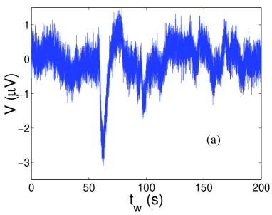
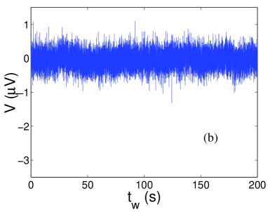
Figure 18: Voltage noise signal in a $2.5\,wt\%$ Laponite sample. (a) Noise signal, 2 hours after the Laponite preparation, when FDT is violated. (b) Typical noise signal when FDT is not violated ($t_{w}=50\,h$).

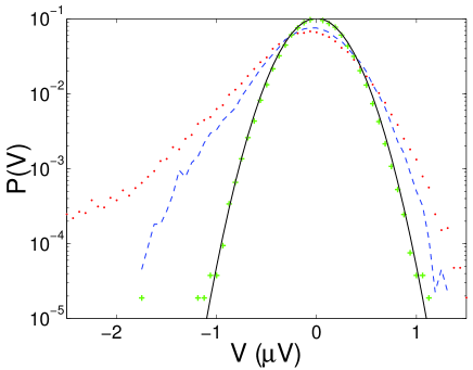
Figure 19: PDF of the voltage noise in a $2.5\,wt\%$ Laponite sample. Typical PDF of the noise signal at different times after preparation, with from top to bottom: $\ (...)t_{w}=1\,h,\ (--)t_{w}=2\,h,\ (+)t_{w}=50\,h$. The continuous line is obtained from the FDT prediction.

As in polycarbonate, the intermittent properties of the noise can be characterized by the PDF of the voltage fluctuations. To compute these distributions, the time series are divided in several time windows and the PDF are computed in each of these window. Afterwards the result of several experiments are averaged. The distributions computed at different times are plotted in Fig. 19. We see that at short $t_{w}$ the PDF presents heavy tails which slowly disappear at longer $t_{w}$. Finally a Gaussian shape is recovered after $t_{w}=16\,h$. This kind of evolution of the PDF clearly indicate that the signal is very intermittent for a young sample and it relaxes to the Gaussian noise at long times.

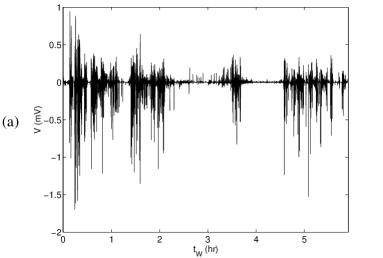
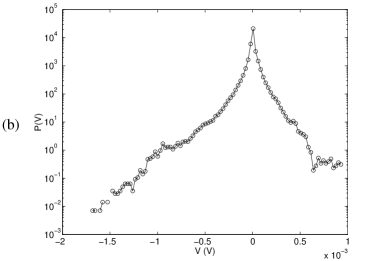
Figure 20: Voltage noise in a $3\,wt\%$ Laponite sample. (a) During the first hours, the voltage noise is dominated by huge intermittent fluctuations: bursts over $1\,mV$ are detected, when thermal noise should present a typical $1\,\mu V$ rms. amplitude. (b) The PDF of this intermittent signal departs clearly from a gaussian distribution.

4.3 Influence of concentration

To check for the influence of concentration on these results, we recently started new series of measurements with $3\,wt\%$ Laponite preparations. In Fig. 20(a) we plot a typical signal measured during the first 6 hours of such a sample. Again, this signal is interrupted by bursts of very large amplitude. As time goes on, the amplitude of the bursts reduces and the time between two consecutive bursts becomes longer and longer. Finally they disappear after a few days, and we only observe classic thermal noise. The main difference with less concentrated samples is in the amplitude and density of this intermittency: now bursts over $1\,mV$ are detected, when thermal noise should present a typical $1\,\mu V$ rms. amplitude, and they are much more frequent. This difference is also clear on the PDF of the signal, plotted in Fig. 20(b). The non gaussian shape is much more pronounced, and the presence of heavy tails clearly indicate that the signal is very intermittent at the beginning of the experiment. In fact, the dynamic is so important that we don’t even have enough precision to resolve the classic thermal fluctuations predicted by the Nyquist formula in this measurement. The influence of increasing the concentration of Laponite preparation thus appears to be somehow similar to the effect of increasing the cooling rate during the quench of the polymer glass: the resulting dynamics is more intermittent in both cases.

4.4 Mechanical noise on Laponite

We have studied the mechanical noise of Laponite in very sensitive thermal rheometer [15] which is based on a principle very similar to the one described for the polycarbonate cantilever in section 3)(see also [47]. We have found that in this case no intermittency is present and the violation of FDT, if it exists, is certainly very small[15]. Recent measurements done on the Brownian motion of a particle inside a Laponite preparation seems to confirm these observations [48].

5 Discussion and conclusions

In the previous sections we have presented several measurements of the electric and mechanical thermal noise in two very different materials: a polymer and a colloidal glass. We first compare the main results on the electric noise measurements which are certainly the most complete. These results are:

• At the very beginning of aging the noise amplitude for both materials is much larger than what predicted by Nyquist relations. In other words Nyquist relations, or more generally FDT, are violated because the materials are out of equilibrium: they are aging. In agreement with theoretical prediction the amplitude and the persistence time of the FDT violation is a decreasing function of frequency and time. The violation is observed even at $\omega t_{w}\gg 1$ and it may last for more than $3h$ for $f>1Hz$.

• The noise slowly relaxes to the usual value after a very long time.

• For the polymer there is a large difference between fast and slow quenches. In the first case the thermal signal is strongly intermittent, in the second case this feature almost disappears. The features of fast and slow quenches in polycarbonate are:

  • After a fast quench the $T_{eff}$ estimated using FDR is huge. This huge $T_{eff}$ is produced by very large intermittent bursts which are at the origin of the low frequency power law decay of noise spectra. The statistic of these events is strongly non Gaussian when FDT is violated and slowly relaxes to a Gaussian one at very long $t_{w}$. The time intervals $\tau$ between two intermittent events are power law distributed with an exponent which depends on $T_{f}$.

  • After a slow quench the $T_{eff}$ estimated using FDR is about $20\%$ larger than $T_{f}$. The intermittency disappears, the noise signal PDF are much closer to a Gaussian and the time between two large fluctuations is not power law distributed.

• The colloidal suspension signal is strongly intermittent, all the more as concentration is increased. The noise signal PDF at small $t_{w}$ is strongly non-Gaussian. The asymmetry of the noise may be linked to the spontaneous polarization of the cell.

We want first to discuss the intermittence of the signal, which has been observed in other aging systems. Our observations are reminiscent of the intermittence observed in the local measurements of polymer dielectric properties [13] and in the slow relaxation dynamics of another colloidal gel [21, 22]. Indeed several theoretical models predict an intermittent dynamics for an aging system. For example the trap model[32] which is based on a phase space description of the aging dynamics. Its basic ingredient is an activation process and aging is associated to the fact that deeper and deeper valleys are reached as the system evolves [23, 24, 25, 26, 27]. The dynamics in this model has to be intermittent because either nothing moves or there is a jump between two traps[23]. This contrasts, for example, with mean field dynamics which is continuous in time[7]. Furthermore two very recent theoretical models predict skewed PDF both for local [51] and global variable [27]. This is a very important observation, because it is worth noticing that one could expect to find intermittency in local variables but not in global. Indeed in macroscopic measurements, fluctuations could be smoothed by the volume average and therefore the PDF would be Gaussian. This is not the case both for our experiments and for the numerical simulations of aging models[27]. In order to push the comparisons with these models of intermittency on a more quantitative level one should analyze more carefully the PDF of the time between events, which is very different in the various models[32, 26, 27]. Our statistics is not yet enough accurate to give clear answers on this point, thus more measurements are necessary to improve the comparisons between theory and experiment. But the time statistics of the trap model [32] seems to fit the data better than that of [26]. The large $T_{eff}$ produced by the intermittent dynamics merits a special comment too. Indeed such a huge $T_{eff}$ is not specific to this class of systems, it has also been observed in domain growth models[10, 49]. The behaviour of these models is however not consistent with that of our system, because in the case of domain growth the huge temperature is given by a weak response, not by an increase of the noise signal.

Going back to the analysis of our experimental data there is another observation, which merits to be discussed. This concerns the difference between fast and slow quenches in polycarbonate. In order to discuss the problem related to this difference it is important to recall that the zero of $t_{w}$ is defined as the instant in which the temperature crosses $T_{g}$. The first question that one may ask, already discussed in section 2.4, is whether the behaviour of the system at the same $t_{w}$ after a slow and a fast quenches is the same. This is certainly not the case because the system takes about $20min$ during a slow quench to reach $T_{f}$ and we have seen that after a fast quench the signal remains intermittent for many hours, whereas after a slow quench intermittency is never observed. Thus one concludes that it is not just a matter of time delay between fast and slow quenches, the dynamics is indeed very different in the two cases. This result can be understood considering that during the fast quench the material is frozen in a state which is highly out of equilibrium at the new temperature. This is not the case for a slow quench. More precisely one may assume that when an aging system is quenched very fast, it explores regions of its phase space that are completely different than those explored in the quasi-equilibrium states of a slow quench. This assumption is actually supported by two recent theoretical results [33, 34], which were obtained in order to give a satisfactory explanation, in the framework of the more recent models, of the old Kovacs effect on the volume expansion[4]. Our results based on the noise measurements can be interpreted in the same way.

Finally, we want to discuss the analogy between the electrical thermal noise in the fast quench experiment of the polymer and that of the gel during the sol-gel transition. In spite of the physical mechanisms that are certainly very different, the statistical properties of the signals are very similar. Thus one may wonder, what is the relationship between the fast quench in the polymer and the gel formation. As already mentioned, during the fast quench the polymer is strongly out of equilibrium, which is the same situation for the liquid-like state at the very beginning of the gel transition. The speed of this transition is controlled by the initial Laponite/water concentration and therefore intermittency should be a function of this parameter. Preliminary measurements seem to confirm this guess: the higher the concentration, the stronger the intermittency.

The main consequence of these observations in the electric measurements is that the definition of $T_{eff}$ based on FDR depends on the cooling rate (on the concentration for the colloid) and probably on $T_{f}$. In fig.21 we have summarized the $T_{eff}$ obtained by electric measurements performed on glycerol[11] and on polycarbonate (Sec.2) and by magnetic measurements performed on a spin glass [16]. Specifically we plot $T_{eff}/T_{g}$ versus $T_{f}/T_{g}$. The straight line is the FDT prediction for $T_{eff}$. Looking at this figure we see that the situation is rather confused. However it becomes more clear if one takes into account the cooling rate. As the $T_{g}$ is quite different in the various materials we define a relative cooling rate $Q={\partial T\over\partial t}{1\over T_{g}}$, which takes the following values: $0.5\ min^{-1}$ for the spin glass, $0.12\ min^{-1}$ for the polycarbonate fast quenches ($T_{f}/T_{g}=0.93$ and $0.79$), $0.009\ min^{-1}$ for the polycarbonate slow quenches ($T_{f}/T_{g}=0.98$) and $0.012\ min^{-1}$ for the glycerol experiment. Thus by considering the relative cooling rate it is clear that in the fast quenches $T_{eff}$ is very large and in the slow quenches it is small independently of the material. However a dependence on $T_{f}$ seems to be present too. Many more measurements are certainly necessary to confirm this dependence of $T_{eff}$ on $T_{f}$ and on the cooling rate.

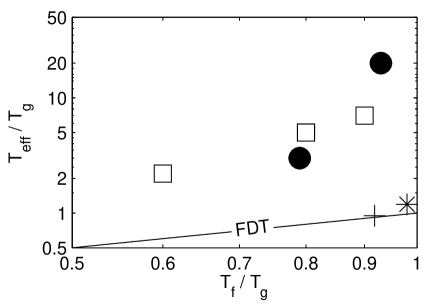
Figure 21: $T_{eff}$ as a function of $T_{f}$. $T_{eff}$ measured in several experiments on different types of glasses at the beginning of the aging regime. (+) glycerol ($f=7Hz$) [11], ($\square$) spin glass ($q=q_{min}$) [16], ($\bullet$) polycarbonate ($f=7Hz$, fast quench), ($*$) polycarbonate ($f=7Hz$, slow quench)

Let us now briefly discuss the results on the mechanical thermal noise. To the best of our knowledge there are only three measurements done on this kind of noise in aging systems, one in polycarbonate (Sec.3) and two in Laponite [15, 48]. The two measurements done in Laponite show that for short $t_{w}$ there is no intermittency and the violation of FDT is very small. Thus in the case of this colloidal glass different observables give different $T_{eff}$. However this result contrasts with the one described in Sec.3 where we have shown that the measurements of the mechanical thermal noise agree with the electric ones because after a fast quench both measurements confirm the presence of a strong intermittency in the aging dynamics of polycarbonate. This comparison between the mechanical and electric measurements in polycarbonate is at the moment rather qualitative due to the difficulty of the mechanical measurements. Much more precise data are certainly necessary to give a clear answer. The difference between the mechanical noise in polycarbonate and in Laponite is still unexplained. It is certainly related with the fact the intermittency in the electrical measurements in Laponite is related to the important role played by the ions in the gel formation.

We want to conclude by a few important and general questions which remain opens. The first concerns the quench rate. Indeed, is it the speed in which $T_{g}$ is crossed that determines the dynamics or the time in which $T_{f}$ is approached ? This question has been already studied in the context of response functions but it will be important to analyze it in terms of noise. The second important open question is why in realistic simulations of Lenard-Jones glasses intermittency has not been observed [52, 53]. Several hypothesis can be done:(i) The simulations are done for a time which is too short to observe intermittency which is a very slow phenomenon. (ii) In the simulation the quench are performed at imposed volume, this is a big difference with respect to the experiments which are done at imposed pressure. A third open question concerns the different dynamics of the thermal noise measured on different observables. Indeed even from a theoretical point view the effective temperature of different observables is the same in certain models [54] and different in others [23]. This is certainly a useful information that can give new insight to the problem of the mechanisms of aging dynamics in different materials.

This lecture clearly shows the importance of associating thermal noise and response measurements. As we have already pointed out in the introduction the standard techniques, based on response measurements and on the application of thermal perturbations to the sample, are certainly important to fix several constrains for the phase space of the system. However they do no give information on the dynamics of the sample, which can be obtained by the study of FDR and of the fluctuation PDF.

Acknowledgments We acknowledge useful discussion with J.L. Barrat, J. P. Bouchaud, S. Franz and J. Kurchan. We thank P. Metz, F. Vittoz and D. Le Tourneau for technical assistance. This work has been partially supported by the DYGLAGEMEM contract of EEC, and by the contract “Vieillissement des matériaux amorphes” of Région Rhône-Alpes.

References

- [1] L.C. Struick, Physical aging in amorphous polymers and other materials (Elsevier, Amsterdam, 1978).
- [2] Spin Glasses and Random Fields, edited by A. P. Young, Series on Directions in Condensed Matter Physics Vol.12 ( World Scientific, Singapore 1998).
- [3] M. Kroon, G. H. Wegdam, and R. Sprik, “Dynamic light scattering studies on the sol-gel transition of a suspension of anisotropic colloidal particles”, Phys. Rev. E 54 , p. 1, 1996.
- [4] A.J. Kovacs, La contraction isotherme du volume des polymères amorphes, Journal of polymer science, 30, p.131-147, (1958).
- [5] K. Jonason, E. Vincent, J. Hamman, J. P. Bouchaud, Memory and chaos effects in spin glasses, Phys. Rev. Lett., 81, 3243 (1998).
- [6] L. Bellon, S. Ciliberto, C. Laroche, Advanced Memory effects in the aging of a polymer glass, Eur. Phys. J. B., 25, 223, (2002).
- [7] L. Cugliandolo, J. Kurchan, Analytical Solution of the Off Equilibrium Dynamics of a Long Range Spin Glass Model, Phys. Rev. Lett., 71, p.173, (1993).
- [8] J.P. Bouchaud, L. F. Cugliandolo, J. Kurchan, M. Mézard, Out of equilibrium dynamics in Spin Glasses and other glassy systems, in Spin Glasses and Random Fields, ed A.P. Young (World Scientific, Singapore 1998). (also in cond-mat/9702070)
- [9] L. Cugliandolo, Effective temperatures out of equilibrium, to appear in Trends in Theoretical Physics II, eds. H Falomir et al, Am. Inst. Phys. Conf. Proc. of the 1998 Buenos Aires meeting, cond-mat/9903250
- [10] L. Cugliandolo, J. Kurchan, L. Peliti, Energy flow, partial equilibration and effective temperatures in systems with slow dynamics, Phys. Rev. E, 55, p.3898 (1997).
- [11] T. S. Grigera, N. Israeloff, Observation of Fluctuation-Dissipation-Theorem Violations in a Structural Glass, Phys. Rev. Lett., 83, p.5038 (1999).
- [12] W.K.Kegel, A.van Blaaderen Direct observation of dynamical heterogeneities in colloïdal hard-sphere suspensions, Science, 287, p.290, (2000).
- [13] E. Vidal Russel, N. E. Israeloff, Direct observation of molecular cooperativity near the glass transition, Nature, 408,695 (2000).
- [14] L. Bellon, S. Ciliberto, C. Laroche, Violation of fluctuation dissipation relation during the formation of a colloidal glass, Europhys. Lett., 53, 511 (2001).
- [15] L.Bellon, S. Ciliberto, Experimental study of fluctuation dissipation relation during the aging process, Physica D, 168, 325 (2002).
- [16] D. Herrisson, M. Ocio, Fluctuation-dissipation ratio of a spin glass in the aging regime, Phys. Rev. Lett., 88, 257702 (2002).
- [17] E.R.Weeks, D.A.Weitz Properties of cage rearrangements observed near the colloidal glass transition, Phys.Rev.Lett., 89, p.95704, (2002).
- [18] L. Buisson, A. Garcimartin, S. Ciliberto, Intermittent origin of the large fluctuation-dissipation relations in an aging polymer glass, Europhys. Lett., 63, p.603, (2003).
- [19] L. Buisson, L. Bellon and S. Ciliberto, Intermittency in aging, J. Phys.: Condens. Matter 15, pp. S1163-S1179, 2003.
- [20] L. Buissn, S.Ciliberto, ”Off equilibrium fluctuations in a polymer glass”, submitted to Physica D, cond-mat/0411252,
- [21] L. Cipelletti, H. Bissig, V. Trappe, P. Ballestat, S. Mazoyer, Direct observation of dynamical heterogeneities in colloïdal hard-sphere suspensions, J. Phys: Condens. Matter, 15, p.S257, (2003).
- [22] H. Bissig, V. Trappe, S. Romer, Luca Cipelletti, Intermittency and non-Gaussian fluctuations in the dynamics of aging colloidal gels, submitted Phys.Rev.Lett.
- [23] S. Fielding, P. Sollich, Observable dependence of Fluctuation dissipation relation and effective temperature, Phys. ReV Lett., 88, 50603-1, (2002).
- [24] A. Perez-Madrid, D. Reguera, J.M. Rubi, Physica A, 329, 357 (2003).
- [25] M. Naspreda, D. Reguera, A. Perez-Madrid, J.M. Rubi, Glassy dynamics: effective temperatures and intermittencies from a two-state model, cond-mat/0411063
- [26] P. Sibani, and J. Dell, Europhys. Lett. 64, p. 8, 2003.
- [27] P. Sibani, H. J. Jensen, Intermittency, aging and record fluctuations,cond-mat/0403212
- [28] C.G. Robertson, G. L. Wilkes, Long term volume relaxation of bisphenol A polycarbonate and atactic polystyrene, Macromolecules 33, 3954 (2000).
- [29] L. Saviot, E. Duval, J.F. Jal, A.J. Dianoux, Very fast relaxation in polycarbonate glass Eur. Phys. J. B., 17 (4), 661, (2000).
- [30] R. Quinson, Caractérisation et modélisation de la déformation non élastique des polymères amorphes à l’état solide,Ph.D. thesis, (INSA), (1998).
- [31] J.P.Bouchaud, Weak ergodicity breaking and aging in disordered systems, J.Phys. I France, 2, p.1705, (1992).
- [32] J.P. Bouchaud, D. S. Dean, Aging on Parisi’s tree, J. Phys. I France, 5, 265 (1995).
- [33] E.M.Bertin, J.P.Bouchaud, J. M. Drouffe, C. Godreche, The Kovacs effect in model glasses, J. Phys. A: Math. Gen 36, 10701 (2003).
- [34] S. Mossa, F. Sciortino, Kovacs effects in aging molecular liquid, Phys. Rev. Lett. 92, 045504 (2004).
- [35] L.D. Landau, E.M. Lifshitz,Theory of Elasticity, 3rd edition, Butterworth-Heinemann (1986)
- [36] N.G. McGrum, B.E. Read, G. Williams, Anelastic and Dielectric Effects in Polymeric Solids, Wiley (1967)
- [37] L.D. Landau, E.M. Lifshitz, Statistical Physics, Part 1, 3rd edition, Butterworth-Heinemann (1980)
- [38] F. Douarche, L. Buisson, S. Ciliberto, A. Petrosyan, A Simple Noise Subtraction Technique, Rev. Scie. Inst., 75,12, 5084 (2004)
- [39] G. Nomarski, Microinterféromètre à ondes polarisées, J. Phys. Radium 16, 9S-16S (1954)
- [40] M. Françon, S. Mallick, Polarization Interferometers, Wiley (1971)
- [41] L. Bellon, S. Ciliberto, H. Boubaker, L. Guyon, Differential interferometry with a complex contrast, Optics Communications 207, 49-56 (2002)
- [42] Laponite RD is a registered trademark of Laporte Absorbents, P.O Box 2, Cheshire, UK.
- [43] D. Bonn, H. Tanaka, G. Wegdam, H. Kellay, and J. Meunier, “Aging of a colloidal ”Wigner” glass,” Europhysics Letters, 45, p. 52, 1999; D. Bonn, H. Kellay, H. Tanaka, G. Wegdam, and J. Meunier, Langmuir, 15, p. 7534, 1999.
- [44] R. Hunter, The foundation of colloid science, Oxford Science Publications, 1989.
- [45] J. Koryta, L. Dvorak and L. Kavan,Principles of Electrochemistry - 2nd Ed., Wiley, 1993.
- [46] H. Nyquist, “Thermal agitation of electrical charge in conductors,” Phys. Rev. 32, pp. 110–113, 1928.
- [47] L. Bellon, L. Buisson, S. Ciliberto, F. Vittoz, Zero applied stress rheometer, Rev. Sci. Instrum. 73, 9, 3286-3290 (2002)
- [48] B. Abou, F. Gallet,Probing an nonequilibrium Einstein relation in an aging colloidal glass, Phys. Rev. Lett., 93, 160603 (2004).
- [49] A. Barrat, Monte-Carlo simulations of the violation of the fluctuation-dissipation theorem in domain growth processes, Phys. Rev.,E57, p. 3629 (1998).
- [50] L. Buisson, M. Ciccotti, L. Bellon, S. Ciliberto,Electrical noise properties in aging materials., In: Fluctuations and Noise in Materials, edited by D. Popovic, M.B. Weissman and Z.A. Racz. Proceedings of SPIE Vol. 5469 (SPIE, Bellingham, WA, 2004). Invited paper. pp. 150-163.
- [51] A. Crisanti, and F. Ritort, Intermittency of Glassy relaxation and the emergence of non-equilibrium spontaneous measure in the aging regime, Europhys. Lett. 66 (2): 253(2004).
- [52] W. Kob, J. L. Barrat, Aging effects in a Lennard Jones Glass, Phys. Rev. Lett., 78, p.4581 (1997);
- [53] J. L. Barrat, W. Kob, Fluctuation dissipation ratio in an aging Lennard-Jones Europhys. Lett., bf 46, p.637 (1999).
- [54] L.Berthier, J.L. Barrat,Shearing a glassy material: Numerical tests of nonequilibrium mode-coupling approaches and experimental proposals, Phys. Rev. Lett., 89, 095702 (2002)