Theory of Transport Properties in the $\mib{p}$-wave Superconducting State of Sr₂RuO₄
- A Microscopic Determination of the Gap Structure -

Abstract

We provide a detailed quantitative analysis of transport properties in the $p$-wave superconducting state of Sr₂RuO₄. Specifically, we calculate ultrasound attenuation rate and electronic thermal conductivity within the mean field approximation. The impurity scattering of the quasi-particles are treated within the self-consistent $T$-matrix approximation, and assumed to be in the unitarity limit. The momentum dependence of the gap function is determined by solving the Eliashberg equation for a three-band Hubbard model with the realistic electronic structure of Sr₂RuO₄. On the basis of the microscopic theory, we can naturally expect nodal structures along the $c$-axis on the cylindrical Fermi surfaces, even if we assume the chiral pairing state (i.e., $\Delta(k)\sim k_{x}\pm{\rm i}k_{y}$). Consequently, we obtain the temperature dependence of the transport coefficients in agreement with the experimental results. We can clarify that actually the thermal excitations on the passively superconducting bands contribute significantly to the thermal conductivity in a wide temperature range, in contrast to the case of other physical quantities.

1 Introduction

The quasi-two-dimensional ruthenate Sr₂RuO₄ has attracted much interest of solid state physicists since the discovery of superconductivity in this compound [1]. A number of excellent experiments and theoretical considerations have already revealed its remarkable and intriguing physical properties. The most important is that Sr₂RuO₄ is a strong candidate of odd-parity spin-triplet superconductor (most likely $p$-wave superconductor) [1, 2, 3], although the crystal structure of Sr₂RuO₄ is the quasi-two-dimensional perovskite structure identical to that of high-$T_{\rm c}$ copper oxides (spin-singlet $d_{x^{2}-y^{2}}$-wave superconductors).

Mechanism of the spin-triplet pairing in Sr₂RuO₄ has been discussed from various microscopic theoretical points of view. In the early stage of the researches, it was considered that some strong ferromagnetic spin fluctuation (Paramagnon) will exist and induce the triplet pairing [4, 5]. However, the inelastic neutron scattering measurement showed that the spin correlation is predominantly incommensurate antiferromagnetic rather than ferromagnetic [6]. Interestingly, some recent theoretical works have shown that the pair-scattering amplitude could actually possess such a characteristic momentum dependence as is favorable for $p$-wave pairing but not attributable to that of the spin susceptibility [7, 8, 9]. These theoretical discussions suggest that the triplet pairing in Sr₂RuO₄ is considered as a natural result from electron correlation, but the essential pairing attraction between the Fermi liquid quasi-particles does not originate from the exchange processes of spin fluctuations [7, 8, 9].

Another interesting problem, which is attacked in the present work, is the detailed clarification of the superconducting gap structure. Superconducting gap structure is closely related to the temperature dependence of physical quantities in general, since the thermal excitations only near the gap minima are essential in responding to various external perturbations. On the theoretical side, the gap structure is a reflection of the momentum dependence of pairing interaction. Therefore, the detailed analyses of the temperature dependence of physical quantities could be a valuable test for the validity of pairing scenario.

The gap structure of Sr₂RuO₄ is still controversial. The most probable pairing symmetry $\Delta(k)\sim(k_{x}\pm{\rm i}k_{y})\hat{z}$ was proposed by Rice and Sigrist very early after the discovery of the superconductivity [4]. The muon spin relaxation experiment [10] suggests strongly that this chiral pairing state, in which the time reversal symmetry is broken, is the most plausible pairing state among several candidates. This pairing symmetry usually results in isotropic gap (i.e., the absence of nodal structure). However, most of existing experimental data exhibit power-law temperature dependence [11, 12, 13, 14, 15, 16], and indicate a nodal gap structure (most probably line nodes) on the Fermi surface. Much effort has been devoted to reconciling these contradictions [17, 18, 19, 20, 21, 22, 23].

In the present article, we analyze microscopically the temperature dependence of two transport coefficients, ultrasound attenuation rate and thermal conductivity, in the superconducting state of Sr₂RuO₄. The sound attenuation rate is expected to provide a strong constraint on the theoretical proposals of superconducting gap structure [24]. We derive the momentum and band dependence of the gap function by solving Eliashberg equation for a realistic tight-binding electronic structure [23]. Starting with a three-band Hubbard model, the effective pairing interaction is evaluated perturbatively to third order in the on-site Coulomb integrals [8]. In our previous works, we showed naturally by this theoretical framework that (i) the momentum dependence of the pairing interaction is favorable for anisotropic $p$-wave pairing, and $p$-wave state is obtained as the most probable pairing state [7, 8], (ii) the superconducting gap possesses line-node-like structures along the $c$-axis [23, 9], and (iii) the calculated specific heat as a function of temperature fits experimental data well [23].

The transport coefficients of Sr₂RuO₄ have been calculated by other authors [25, 26, 28, 27, 29, 30]. Most of them are based on simplified isotropic Fermi surfaces (two- or three-dimensional), or simple gap functions described by one or a few harmonic functions. However, as discussed in the present article, such simplified electronic structures and gap structures are generally insufficient to discuss the experimental data of transport properties.

For the calculation of the transport coefficients, we take the way of analysis which has been developed for some uranium compound superconductors [31, 32, 33]: the non-magnetic impurity scattering is treated by the self-consistent $T$-matrix approximation. The scattering is assumed to be in the unitarity limit. We ignore the vertex corrections. In contrast to the analyses for uranium compounds (where they considered simplified electronic structures, e.g., isotropic spherical Fermi surfaces), we take more realistic tight-binding electronic structure and gap structure for Sr₂RuO₄.

For the calculation of ultrasound attenuation rate, we adopt the same way as Walker and collaborators did [34]. In the work by Walker et al., they succeeded in explaining the large in-plane anisotropy of the attenuation rate, and clarified that the anisotropy of the electron-phonon interaction is essential. This successful point is taken into account also in our present work. However, it should be noted that their gap structure is quite different from ours. They insisted that there should be point nodes on the Fermi surfaces [30]. Although we discuss based on the purely two-dimensional model, we consider that it is almost impossible to obtain point nodes or horizontal (i.e., parallel to the basal plane) line nodes. This is because the pair scattering amplitude can acquire only negligible momentum dependence along the $c$-axis, due to the strong two-dimensionality.

Consequently, we obtain a consistency with the experimental data of the transport coefficients in the overall temperature range. The electron-phonon coupling constants are essential parameters for the good fitting to the experimental data. In addition, the anisotropy due to the lattice structure is also an essential ingredient for reproducing the thermal conductivity and the anisotropy of sound attenuation. Therefore the naive conjectures from the isotropic models and simplified gap functions are not reliable in general.

The present article is constructed as follows. In § 2, the theoretical formulation is given. We give the analytic expressions of ultrasound attenuation rate and thermal conductivity. In § 3, the numerical result of calculated gap structure is provided, and then the numerical results of the ultrasound attenuation rate and thermal conductivity are compared with the experimental data. In § 4, some remarks on our results are given. In addition, relations of the present work with other works are discussed. Finally, in § 5, we will give concluding remarks.

2 Theoretical Formulation

2.1 Three-band Hubbard model and Eliashberg equation

The Fermi surface and the electronic structure of Sr₂RuO₄ near the Fermi level are well reproduced by tight-binding fitting [35]. Since the electronic density of states near the Fermi level is dominated by the partial density of states of Ru4d$\varepsilon$ orbitals [35, 36], the hopping parameters are considered to describe the transfers between the Ru4d$\varepsilon$-like Wannier orbitals. We take the following non-interacting Hamiltonian (these Wannier orbitals are characterized by $\ell=\{xy,\,yz,\,xz\}$):

$$H_{0} = \sum_{\mib{k},\ell,\sigma}\xi_{\ell}(\mib{k})c_{\mib{k}\ell\sigma}^{{\dagger}}c_{\mib{k}\ell\sigma}$$ (1)

$$+\sum_{\mib{k},\sigma}\lambda(\mib{k})(c_{\mib{k}\,yz\,\sigma}^{{\dagger}}c_{\mib{k}\,xz\,\sigma}+c_{\mib{k}\,xz\,\sigma}^{{\dagger}}c_{\mib{k}\,yz\,\sigma}),$$

where $c_{\mib{k}\ell\sigma}$[$c_{\mib{k}\ell\sigma}^{{\dagger}}$] is the electron annihilation[creation] operator (the pseudo-momentum, orbital and spin states are denoted by $\mib{k}$, $\ell$ and $\sigma$, respectively), and the energy dispersions are

$$\xi_{xy}(\mib{k}) = 2t_{1}(\cos k_{x}+\cos k_{y})$$ (2)

$$+4t_{2}\cos k_{x}\cos k_{y}-\mu_{xy},$$

$$\xi_{yz}(\mib{k}) = 2t_{3}\cos k_{y}+2t_{4}\cos k_{x}-\mu_{yz},$$ (3)

$$\xi_{xz}(\mib{k}) = 2t_{3}\cos k_{x}+2t_{4}\cos k_{y}-\mu_{xz},$$ (4)

$$\lambda(\mib{k}) = 4t_{5}\sin k_{x}\sin k_{y}.$$ (5)

In the present work, we take the parameter set $t_{1}=-1.00$, $t_{2}=-0.395$, $t_{3}=-1.25$, $t_{4}=-0.125$, $t_{5}=-0.150$ [37], to reproduce the Fermi surface topology. The chemical potentials $\mu_{\ell}$’s are determined by the condition $n_{\ell}=0.667$, where $n_{\ell}$ is the electron number of orbital $\ell$ per one spin state (The orbitals are evenly filled with electron). We introduce the Coulomb interaction part:

$$H^{\prime} = \frac{U}{2}\sum_{i}\sum_{\ell}\sum_{\sigma\neq\sigma^{\prime}}c_{i\ell\sigma}^{{\dagger}}c_{i\ell\sigma^{\prime}}^{{\dagger}}c_{i\ell\sigma^{\prime}}c_{i\ell\sigma}$$ (6)

$$+\frac{U^{\prime}}{2}\sum_{i}\sum_{\ell\neq\ell^{\prime}}\sum_{\sigma,\sigma^{\prime}}c_{i\ell\sigma}^{{\dagger}}c_{i\ell^{\prime}\sigma^{\prime}}^{{\dagger}}c_{i\ell^{\prime}\sigma^{\prime}}c_{i\ell\sigma}$$

$$+\frac{J}{2}\sum_{i}\sum_{\ell\neq\ell^{\prime}}\sum_{\sigma,\sigma^{\prime}}c_{i\ell\sigma}^{{\dagger}}c_{i\ell^{\prime}\sigma^{\prime}}^{{\dagger}}c_{i\ell\sigma^{\prime}}c_{i\ell^{\prime}\sigma}$$

$$+\frac{J^{\prime}}{2}\sum_{i}\sum_{\ell\neq\ell^{\prime}}\sum_{\sigma\neq\sigma^{\prime}}c_{i\ell\sigma}^{{\dagger}}c_{i\ell\sigma^{\prime}}^{{\dagger}}c_{i\ell^{\prime}\sigma^{\prime}}c_{i\ell^{\prime}\sigma},$$

where the operator $c_{i\ell\sigma}$[$c_{i\ell\sigma}^{{\dagger}}$] is the electron annihilation[creation] operator at $i$-th Ru site ($c_{\mib{k}\ell\sigma}$ is the Fourier transform of $c_{i\ell\sigma}$). The microscopic origin of $H^{\prime}$ is the Coulomb interaction between the Ru4d electrons. The total Hamiltonian is $H=H_{0}+H^{\prime}$.

As we will see in the next section, the Fermi surface consists of three branches (which are named $\alpha$, $\beta$ and $\gamma$), consistent with the de Haas-van Alphen oscillation [38] and photoemission measurements [39]. The Hamiltonian $H_{0}$ is diagonalized easily, and the obtained dispersions are

$$\xi_{\alpha}(\mib{k}) = \xi_{+}(\mib{k})-\sqrt{\xi_{-}^{2}(\mib{k})+\lambda^{2}(\mib{k})},$$ (7)

$$\xi_{\beta}(\mib{k}) = \xi_{+}(\mib{k})+\sqrt{\xi_{-}^{2}(\mib{k})+\lambda^{2}(\mib{k})},$$ (8)

$$\xi_{\gamma}(\mib{k}) = \xi_{xy}(\mib{k}),$$ (9)

where $\xi_{\pm}(\mib{k})=(\xi_{yz}(\mib{k})\pm\xi_{xz}(\mib{k}))/2$. The elements of diagonalization matrix are

$$U(\mib{k})=\begin{array}[]{r@{}l}&\begin{array}[]{ccc}\makebox[6.00006pt]{}\gamma&\makebox[11.00008pt]{}\alpha&\makebox[18.99995pt]{}\beta\end{array}\\ \begin{array}[]{l}{\it xy}\\ {\it yz}\\ {\it xz}\\ \end{array}&\left[\begin{array}[]{ccc}1&0&0\\ 0&K(\mib{k})&L(\mib{k})\\ 0&-L(\mib{k})&K(\mib{k})\end{array}\right],\end{array}$$ (10)

where $K(\mib{k})=\sqrt{(1-M(\mib{k}))/2}$,
$L(\mib{k})={\rm sgn}(\lambda(\mib{k}))\sqrt{(1+M(\mib{k}))/2}$, and $M(\mib{k})=\xi_{-}(\mib{k})/\sqrt{\xi_{-}^{2}(\mib{k})+\lambda^{2}(\mib{k})}$. We define the bare Green’s function:

$$G_{a}^{(0)}(k)=({\rm i}\omega_{n}-\xi_{a}(\mib{k}))^{-1},$$ (11)

the band index $a$ takes $\alpha$, $\beta$ and $\gamma$.

The anomalous self-energy (i.e., superconducting order parameter) is obtained by solving the linearized Eliashberg equation:

$$\Sigma_{a,\sigma_{1}\sigma_{2}}^{\rm A}(k)=-\frac{T}{N}\sum_{a^{\prime},k^{\prime},\sigma_{3}\sigma_{4}}V_{a\sigma_{1}\sigma_{2},a^{\prime}\sigma_{3}\sigma_{4}}(k,k^{\prime})$$

$$\times|G_{a^{\prime}}^{(0)}(k^{\prime})|^{2}\Sigma_{a^{\prime},\sigma_{4}\sigma_{3}}^{\rm A}(k^{\prime}),$$ (12)

where $k^{(}{}^{\prime}{}^{)}=(\mib{k}{}^{(}{}^{\prime}{}^{)},{\rm i}\omega_{n}{}^{(}{}^{\prime}{}^{)})$ [$\omega_{n}=(2n+1)\pi T$], and band index $a^{(}{}^{\prime}{}^{)}$ takes $\alpha$, $\beta$ and $\gamma$. The effective interaction $V_{a\sigma_{1}\sigma_{2},a^{\prime}\sigma_{3}\sigma_{4}}(k,k^{\prime})$ is evaluated by the third order perturbation expansion in $H^{\prime}$. In the present calculation, we take $U=4.0$, $U^{\prime}=0.33U$, $J=0.33U$, $J^{\prime}=0.33U$. The lengthy procedure of expansions and the numerical solutions of the Eliashberg equation (12) are given in the previous work [8]. For the spin-triplet states, the order parameter is expressed using the vectorial notation: $\Sigma_{a,\sigma_{1}\sigma_{2}}^{\rm A}(k)=[{\rm i}(\mib{D}_{a}(k)\cdot\mib{\sigma})\sigma_{y}]_{\sigma_{1}\sigma_{2}}$.

We assume that the momentum and temperature dependence of the superconducting gap function $\Delta_{a}(\mib{k})$ are given by the following equation (as in ref. References),

$$\Delta_{a}(\mib{k})=f_{a}(\mib{k})\Delta(T),$$ (13)

where $f_{a}(\mib{k})={\rm Const.}\times D_{a}(k)$, and $D_{a}(k)$ is the component of the vector $\mib{D}_{a}(k)$ (we assume $\mib{D}_{a}(k)=D_{a}(k)\hat{z}$.), and obtained by solving the above Eliashberg equation (12). The temperature dependence of the gap magnitude $\Delta(T)$ is determined by the standard BCS gap equation:

$$\Delta_{a}(\mib{k})=-\frac{1}{N}\sum_{a^{\prime},\mib{k}^{\prime}}V_{\mib{k}a,\mib{k}^{\prime}a^{\prime}}\frac{\tanh[E_{a^{\prime}}(\mib{k}^{\prime})/(2T)]}{E_{a^{\prime}}(\mib{k}^{\prime})}\Delta_{a^{\prime}}(\mib{k}^{\prime}),$$ (14)

with $V_{\mib{k}a,\mib{k}^{\prime}a^{\prime}}=-f_{a}(\mib{k})f_{a^{\prime}}^{*}(\mib{k}^{\prime})$ and $E_{a}(\mib{k})=\sqrt{\xi_{a}^{2}(\mib{k})+|\Delta_{a}(\mib{k})|^{2}}$. $f_{a}(\mib{k})$ is an odd-parity function, satisfying the relation $f_{a}(\mib{k})=-f_{a}(-\mib{k})$. We assume the chiral state is realized:

$$f_{a}(\mib{k})=f_{a}^{x}(\mib{k})\pm{\rm i}f_{a}^{y}(\mib{k}),$$ (15)

where $f_{a}^{x}(\mib{k})$[$f_{a}^{y}(\mib{k})$] is a real function possessing the $k_{x}$-like[$k_{y}$-like] symmetry. The superconducting gap structure on band $a$ is obtained by the absolute magnitude of $\Delta_{a}(\mib{k})$,

$$|\Delta_{a}(\mib{k})|=|f_{a}(\mib{k})|\Delta(T)=\sqrt{{f_{a}^{x}(\mib{k})}^{2}+{f_{a}^{y}(\mib{k})}^{2}}\Delta(T).$$ (16)

For the details of the discussions in this section, one could refer to refs. References and References.

2.2 Self-consistent $T$-matrix approximation for non-magnetic impurity scattering

Here we consider non-magnetic impurity scattering, as preliminaries for the following discussions on transport properties:

$$H_{\rm imp}=\sum_{j\in{\rm imp.}}\sum_{\ell\ell^{\prime}\sigma}u_{\ell\ell^{\prime}}c_{j\ell\sigma}^{{\dagger}}c_{j\ell^{\prime}\sigma}.$$ (17)

“$j\in{\rm imp.}$” means that the summation is performed over the impurity positions. The impurities are randomly positioned at Ru sites. We assume simply $u_{\ell\ell^{\prime}}=u\delta_{\ell\ell^{\prime}}$, because of the symmetry properties of the Ru4d$\varepsilon$ orbital wave functions. In addition, we assume that $u$ is much larger than the band width $W$ ($u>100W$ for the numerical calculations), i.e., the scattering is almost in the unitarity limit.

In order to discuss the effect of impurities, we take the standard $T$-matrix approximation [40]. The self-energy for the impurity scattering is given by

$$\Sigma_{\ell\ell^{\prime}}({\rm i}\omega_{n})=cT_{\ell\ell^{\prime}}({\rm i}\omega_{n}).$$ (18)

$c$ is the impurity concentration, and we take $c=10^{-6}$ for the present work. $T_{\ell\ell^{\prime}}({\rm i}\omega_{n})$ is the $T$-matrix obtained by solving the equation,

$$T_{\ell\ell^{\prime}}({\rm i}\omega_{n})=u_{\ell\ell^{\prime}}+\frac{1}{N}\sum_{\mib{k}_{1},\ell_{1}\ell_{2}}u_{\ell\ell_{1}}G_{\ell_{1}\ell_{2}}(\mib{k}_{1},{\rm i}\omega_{n})T_{\ell_{2}\ell^{\prime}}({\rm i}\omega_{n}),$$ (19)

where $G_{\ell\ell^{\prime}}(k)$ is the Green’s function. We have already omitted the terms containing $\sum_{\mib{k}}F_{\ell\ell^{\prime}}(k)$ [$F_{\ell\ell^{\prime}}(k)$ is the anomalous Green’s function. See below.], which vanish in non-$s$-wave superconducting states [42], in contrast to the case of $s$-wave superconducting state. The impurity self-energy and Green’s functions are related by the Gorkov equation:

$$G_{a}(k) = G_{a}^{(0)}(k)+G_{a}^{(0)}(k)\Sigma_{a}(k)G_{a}(k)$$ (20)

$$-G_{a}^{(0)}(k)\Delta_{a}(\mib{k})F_{a}^{{\dagger}}(k),$$

$$F_{a}(k) = G_{a}^{(0)}(k)\Sigma_{a}(k)F_{a}(k)$$ (21)

$$+G_{a}^{(0)}(k)\Delta_{a}(\mib{k})G_{a}(-k),$$

$$F_{a}^{{\dagger}}(k) = G_{a}^{(0)}(-k)\Sigma_{a}(-k)F_{a}^{{\dagger}}(k)$$ (22)

$$+G_{a}^{(0)}(-k)\Delta_{a}^{*}(\mib{k})G_{a}(k).$$

Using the matrix $U(\mib{k})$ in eq. (10), the orbital indices $\ell{}^{(}{}^{\prime}{}^{)}$ in $\Sigma_{\ell\ell^{\prime}}({\rm i}\omega_{n})$ are converted to band index $a$ by

$$\Sigma_{a}(k) = \sum_{\ell\ell^{\prime}}U_{a\ell}^{{\dagger}}(\mib{k})U_{\ell^{\prime}a}(\mib{k})\Sigma_{\ell\ell^{\prime}}({\rm i}\omega_{n}),$$ (23)

and the band index $a$ in the Green’s functions are converted to the orbital indices $\ell{}^{(}{}^{\prime}{}^{)}$ by

$$G_{\ell\ell^{\prime}}(k) = \sum_{a}U_{\ell a}(\mib{k})U_{a\ell^{\prime}}^{{\dagger}}(\mib{k})G_{a}(k),$$ (24)

$$F_{\ell\ell^{\prime}}(k) = \sum_{a}U_{\ell a}(\mib{k})U_{\ell^{\prime}a}(\mib{k})F_{a}(k),$$ (25)

$$F_{\ell\ell^{\prime}}(k) = \sum_{a}U_{a\ell}^{{\dagger}}(\mib{k})U_{a\ell^{\prime}}^{{\dagger}}(\mib{k})F_{a}^{{\dagger}}(k).$$ (26)

Defining the renormalized Green’s function by

$$\bar{G}_{a}(k) = ({G_{a}^{(0)}}^{-1}(k)-\Sigma_{a}(k))^{-1}$$ (27)

$$= ({\rm i}\omega_{n}-\xi_{a}(\mib{k})-\Sigma_{a}(k))^{-1},$$

the above Gorkov’s equation is simplified to

$$G_{a}(k) = \bar{G}_{a}(k)-\bar{G}_{a}(k)\Delta_{a}(\mib{k})F_{a}^{{\dagger}}(k),$$ (28)

$$F_{a}(k) = \bar{G}_{a}(k)\Delta_{a}(\mib{k})G_{a}(-k),$$ (29)

$$F_{a}^{{\dagger}}(k) = \bar{G}_{a}(-k)\Delta_{a}^{*}(\mib{k})G_{a}(k).$$ (30)

By solving eqs. (28)-(30), the Green’s functions are obtained:

$$G_{a}(k) = \frac{1}{\bar{G}_{a}^{-1}(k)+\bar{G}_{a}^{*}(k)|\Delta_{a}(\mib{k})|^{2}},$$ (31)

$$F_{a}(k) = \frac{\Delta_{a}(\mib{k})}{|\bar{G}_{a}(k)|^{-2}+|\Delta_{a}(\mib{k})|^{2}},$$ (32)

$$F_{a}^{{\dagger}}(k) = \frac{\Delta_{a}^{*}(\mib{k})}{|\bar{G}_{a}(k)|^{-2}+|\Delta_{a}(\mib{k})|^{2}}.$$ (33)

We continue this expression analytically to the real frequency axis (${\rm i}\omega_{n}\rightarrow z+{\rm i}0$):

$$G_{a}^{\rm R}(k) =$$

$$\frac{\tilde{z}_{a}^{{\rm R}*}(-k)-\xi_{a}(\mib{k})}{(\tilde{z}_{a}^{\rm R}(k)-\xi_{a}(\mib{k}))(\tilde{z}_{a}^{{\rm R}*}(-k)-\xi_{a}(\mib{k}))+|\Delta_{a}(\mib{k})|^{2}},$$

$$F_{a}^{\rm R}(k) =$$

$$\frac{\Delta_{a}(\mib{k})}{(\tilde{z}_{a}^{\rm R}(k)-\xi_{a}(\mib{k}))(\tilde{z}_{a}^{{\rm R}*}(-k)-\xi_{a}(\mib{k}))+|\Delta_{a}(\mib{k})|^{2}},$$

$$F_{a}^{{\dagger}{\rm R}}(k) =$$

$$\frac{\Delta_{a}^{*}(\mib{k})}{(\tilde{z}_{a}^{\rm R}(k)-\xi_{a}(\mib{k}))(\tilde{z}_{a}^{{\rm R}*}(-k)-\xi_{a}(\mib{k}))+|\Delta_{a}(\mib{k})|^{2}},$$

with

$$\tilde{z}_{a}^{\rm R}(k)=z-\Sigma_{a}^{\rm R}(k),$$ (37)

and $k=(\mib{k},z)$. Here we may assume the electron-hole symmetry in order to simplify the discussion, although the actual electronic structure does not possess the symmetry. This simplification does not affect the results, since the temperatures we consider here are enough low, compared with the characteristic energy scale of the asymmetric structure of the density of states. Under the electron-hole symmetry, we have the relation $\tilde{z}_{a}^{{\rm R}*}(-k)=-\tilde{z}_{a}^{\rm R}(k)$, and the expressions are simplified to

$$G_{a}^{\rm R}(k) = \frac{\tilde{z}_{a}^{\rm R}(k)+\xi_{a}(\mib{k})}{{\tilde{z}_{a}^{\rm R}(k)}^{2}-{\xi_{a}(\mib{k})}^{2}-|\Delta_{a}(\mib{k})|^{2}},$$ (38)

$$F_{a}^{\rm R}(k) = -\frac{\Delta_{a}(\mib{k})}{{\tilde{z}_{a}^{\rm R}(k)}^{2}-{\xi_{a}(\mib{k})}^{2}-|\Delta_{a}(\mib{k})|^{2}},$$ (39)

$$F_{a}^{{\dagger}{\rm R}}(k) = -\frac{\Delta_{a}^{*}(\mib{k})}{{\tilde{z}_{a}^{\rm R}(k)}^{2}-{\xi_{a}(\mib{k})}^{2}-|\Delta_{a}(\mib{k})|^{2}}.$$ (40)

We determine $\tilde{z}_{a}^{\rm R}(k)$, by solving simultaneously the analytically continued forms of eqs. (18), (19), (23) and (24), and eqs. (37), (38). There we use $\Delta_{a}(\mib{k})$ derived in the absence of the impurities (in § 2.1). This means that the changes of the gap function and its temperature dependence due to the impurities are neglected in the present study. We consider that the impurity concentration $c$($=10^{-6}$) is enough small not to change significantly the gap structure and its temperature dependence.

In the present work, we assume that the damping of thermally excited quasi-particles is dominantly caused by the impurity scattering, and ignore the damping effect due to electron-electron scattering. We could justify the assumption as follows. Within a simple discussion, we expect the normal-state electronic thermal conductivity $\kappa_{\rm n}$ behaves at low temperatures as

$$\kappa^{-1}_{\rm n}\sim dT^{-1}+fT+gT^{2},$$ (41)

where $T$ is temperature, and $d$, $f$ and $g$ are constants [41]. The first, second and third terms of the right hand side in eq. (41) originate from the impurity scattering, the electron-electron scattering and the electron-phonon scattering, respectively. According to the experimental data of the normal-state thermal conductivity in ref. References, we find that the first term is sufficiently larger than the other two terms within the low-temperature region.

2.3 Ultrasound attenuation rate

Scattering of phonons by the electron system causes the ultrasound attenuation. We consider the electron-phonon interaction:

$$H_{\rm ep}=N^{-\frac{1}{2}}\sum_{\mib{k}\mib{q},\ell\ell^{\prime},\sigma}\Lambda_{\mib{k},\mib{q},\ell\ell^{\prime}}\phi_{\mib{q}}c_{\mib{k}+\mib{q}\ell\sigma}^{{\dagger}}c_{\mib{k}\ell^{\prime}\sigma},$$ (42)

where $\phi_{\mib{q}}=b_{\mib{q}}+b_{\mib{-q}}^{{\dagger}}$, and $b_{\mib{q}}$($b_{\mib{q}}^{{\dagger}}$) is the phonon annihilation(creation) operator with momentum $\mib{q}$. The matrix elements $\Lambda_{\mib{k},\mib{q},\ell\ell^{\prime}}$ for the present electronic structure of Sr₂RuO₄ are given by

$$\Lambda_{\mib{k},\mib{q},xy,xy} = {\rm i}\{\tilde{g}_{1}(\cos k_{x}\hat{e}_{x}\hat{q}_{x}+\cos k_{y}\hat{e}_{y}\hat{q}_{y})$$ (43)

$$+\tilde{g}_{2}\cos k_{x}\cos k_{y}(\hat{e}_{x}\hat{q}_{x}+\hat{e}_{y}\hat{q}_{y})$$

$$-\tilde{g}_{2}\sin k_{x}\sin k_{y}(\hat{e}_{x}\hat{q}_{y}+\hat{e}_{y}\hat{q}_{x})\},$$

$$\Lambda_{\mib{k},\mib{q},yz,yz} = {\rm i}(\tilde{g}_{4}\cos k_{x}\hat{e}_{x}\hat{q}_{x}+\tilde{g}_{3}\cos k_{y}\hat{e}_{y}\hat{q}_{y}),$$ (44)

$$\Lambda_{\mib{k},\mib{q},xz,xz} = {\rm i}(\tilde{g}_{3}\cos k_{x}\hat{e}_{x}\hat{q}_{x}+\tilde{g}_{4}\cos k_{y}\hat{e}_{y}\hat{q}_{y}),$$ (45)

$$\Lambda_{\mib{k},\mib{q},yz,xz} = \Lambda_{\mib{k},\mib{q},xz,yz}$$ (46)

$$= {\rm i}\tilde{g}_{5}\{-\sin k_{x}\sin k_{y}(\hat{e}_{x}\hat{q}_{x}+\hat{e}_{y}\hat{q}_{y})$$

$$+\cos k_{x}\cos k_{y}(\hat{e}_{x}\hat{q}_{y}+\hat{e}_{y}\hat{q}_{x})\},$$

and the other elements are zero (See Appendix A). $\hat{\mib{e}}=(\hat{e}_{x},\hat{e}_{y})$ and $\hat{\mib{q}}=(\hat{q}_{x},\hat{q}_{y})$ are the unit vectors along the directions of phonon polarization and phonon propagation, respectively.

The energy spectrum of phonon is given by the poles of phonon Green’s function. The phonon Green’s function $D(q)$ [$q=(\mib{q},{\rm i}\Omega_{m})$, $\Omega_{m}=2m\pi T$] satisfies

$$D(q)=D^{(0)}(q)+D^{(0)}(q)\Pi(q)D(q),$$ (47)

where $D^{(0)}(q)$ is the bare phonon Green’s function [$D^{(0)}(q)=-2\omega_{0}(\mib{q})/({\Omega_{m}}^{2}+{\omega_{0}}(\mib{q})^{2})$], and $\Pi(q)$ is the phonon self-energy. Using the retarded phonon Green’s function $D^{R}(q)$ [$D^{R}(q)$ is the analytic continuation of $D(q)$ to the real axis by ${\rm i}\Omega_{m}\to\Omega+{\rm i}0$ $(m>0)$], the attenuation rate $\alpha$ of the phonon with momentum $\mib{q}$ is obtained by solving ${D^{R}(\mib{q},\Omega)}^{-1}=0$ for $\Omega$ and then taking the imaginary part of the solution: $\alpha\equiv{\rm Im}\Omega\approx-{\rm Im}\Pi^{R}(\mib{q},\omega_{0}(\mib{q}))$. $\Pi^{R}(\mib{q},\Omega)$ is the analytic continuation of $\Pi(\mib{q},{\rm i}\Omega_{m})$. The phonon self-energy $\Pi(q)$ within the mean field theory is represented by the diagrams in Fig. 1.

Figure 1: The diagrammatic representation of the phonon self-energy part within the mean field approximation. The solid lines with arrowheads denote the Green’s functions.

The analytic expression of the phonon self-energy is

$$\Pi(q)=2\frac{T}{N}\sum_{k,\ell_{i}}\Lambda_{\mib{k},-\mib{q},\ell_{1}\ell_{2}}\Lambda_{\mib{k},\mib{q},\ell_{3}\ell_{4}}$$

$$\times[G_{\ell_{2}\ell_{3}}(k+q)G_{\ell_{4}\ell_{1}}(k)-F_{\ell_{1}\ell_{3}}^{{\dagger}}(k+q)F_{\ell_{4}\ell_{2}}(k)],$$ (48)

where we have used the relation $\Lambda_{-\mib{k},\mib{q},\ell\ell^{\prime}}=\Lambda_{\mib{k},\mib{q},\ell\ell^{\prime}}$, and the approximate relation $\Lambda_{\mib{k}+\nu\mib{q},\mib{q},\ell\ell^{\prime}}\approx\Lambda_{\mib{k},\mib{q},\ell\ell^{\prime}}$ (for $\nu\sim 1$) within the precision to the leading order of $|\mib{q}|$. The front factor two originates from the summation with respect to spin indices. We continue $\Pi(q)$ analytically to the real axis, convert orbital indices $\ell_{i}$ to band index $a$, and take the imaginary part. Since we consider the hydrodynamic limit ($\ell_{\rm e}\ll 2\pi/|\mib{q}|$, $\ell_{\rm e}$: mean free path) in the present study, we may take the limit $\mib{q},\Omega\rightarrow 0$ in the argument of the Green’s functions. Thus we obtain the expression for the attenuation rate $\alpha$:

$$\alpha=\frac{\omega_{0}(\mib{q})}{2\pi T}\sum_{a,\mib{k}}|\Lambda_{\mib{k},\mib{q},a}|^{2}\int_{-\infty}^{\infty}{\rm d}z\frac{1}{\cosh^{2}(\frac{z}{2T})}$$

$$\times\bigl{[}({\rm Im}G_{a}^{\rm R}(\mib{k},z))^{2}-|\Delta_{a}(\mib{k})|^{2}({\rm Im}\tilde{F}_{a}^{\rm R}(\mib{k},z))^{2}\bigr{]},$$ (49)

where $\tilde{F}_{a}^{\rm R}(\mib{k},z)$ is defined by $F_{a}^{\rm R}(\mib{k},z)=\Delta_{a}(\mib{k})\tilde{F}_{a}^{\rm R}(\mib{k},z)$, and we have neglected the inter-band crossing terms, ${\rm Im}G_{a}(k){\rm Im}G_{a^{\prime}}(k)$ and ${\rm Im}F_{a}(k){\rm Im}F_{a^{\prime}}(k)$ ($a\neq a^{\prime}$). The contribution from these crossing terms is considered to be negligibly small in the present case of the long-wavelength limit and low temperatures. $\Lambda_{\mib{k},\mib{q},a}$ is related to $\Lambda_{\mib{k},\mib{q},\ell\ell^{\prime}}$ by

$$\Lambda_{\mib{k},\mib{q},a}=\sum_{\ell_{1}\ell_{2}}U_{a\ell_{1}}^{{\dagger}}(\mib{k})U_{\ell_{2}a}(\mib{k})\Lambda_{\mib{k},\mib{q},\ell_{1}\ell_{2}}.$$ (50)

Here we perform the momentum integration perpendicular to the Fermi surfaces in eq. (49). Using the expressions of the Green’s functions (38) and (39), and adopting the approximate form of integration measure,

$$\sum_{a,\mib{k}}\cdots\rightarrow\sum_{a,\mib{k}_{\rm F}}\biggl{|}\frac{\partial\xi_{a}(\mib{k})}{\partial\mib{k}}\biggr{|}^{-1}_{{\mib k}={\mib k}_{\rm F}}\int_{-\infty}^{\infty}{\rm d}\xi_{a}\cdots,$$ (51)

the formula (49) is reduced to

$$\alpha=\frac{\omega_{0}(\mib{q})}{2\pi T}\sum_{a,\mib{k}_{\rm F}}|\Lambda_{\mib{k}_{\rm F},\mib{q},a}|^{2}\biggl{|}\frac{\partial\xi_{a}(\mib{k})}{\partial\mib{k}}\biggr{|}^{-1}_{{\mib k}={\mib k}_{\rm F}}\int_{-\infty}^{\infty}{\rm d}z\int_{-\infty}^{\infty}{\rm d}\xi_{a}$$

$$\times\frac{1}{\cosh^{2}(\frac{z}{2T})}\biggl{[}\biggl{(}{\rm Im}\frac{\tilde{z}_{a}^{\rm R}(\mib{k}_{\rm F},z)+\xi_{a}}{{\tilde{z}_{a}^{\rm R}(\mib{k}_{\rm F},z)}^{2}-{\xi_{a}}^{2}-|\Delta_{a}(\mib{k}_{\rm F})|^{2}}\biggr{)}^{2}$$

$$-\biggl{(}{\rm Im}\frac{|\Delta_{a}(\mib{k}_{\rm F})|}{{\tilde{z}_{a}^{\rm R}(\mib{k}_{\rm F},z)}^{2}-{\xi_{a}}^{2}-|\Delta_{a}(\mib{k}_{\rm F})|^{2}}\biggr{)}^{2}\biggr{]}.$$

(52)

$\sum_{\mib{k}_{\rm F}}$ means the momentum integration on the Fermi surface. We obtain the final expression of $\alpha$ by performing the integration with respect to $\xi_{a}$:

$$\alpha=\frac{\omega_{0}(\mib{q})}{8T}\sum_{a,\mib{k}_{\rm F}}|\Lambda_{\mib{k}_{\rm F},\mib{q},a}|^{2}\int_{-\infty}^{\infty}{\rm d}z\frac{1}{\cosh^{2}(\frac{z}{2T})}I_{a}(\mib{k}_{\rm F},z),$$ (53)

with

$$I_{a}(\mib{k}_{\rm F},z) = \biggl{|}\frac{\partial\xi_{a}(\mib{k})}{\partial\mib{k}}\biggr{|}^{-1}_{{\mib k}={\mib k}_{\rm F}}$$ (54)

$$\times \frac{1}{{\rm Im}\sqrt{{\tilde{z}_{a}^{\rm R}(\mib{k}_{\rm F},z)}^{2}-|\Delta_{a}(\mib{k}_{\rm F})|^{2}}}$$

$$\times \biggl{(}1+\frac{|\tilde{z}_{a}^{\rm R}(\mib{k}_{\rm F},z)|^{2}-|\Delta_{a}(\mib{k}_{\rm F})|^{2}}{|{\tilde{z}_{a}^{\rm R}(\mib{k}_{\rm F},z)}^{2}-|\Delta_{a}(\mib{k}_{\rm F})|^{2}|}\biggr{)}.$$

The electron-phonon coupling $\Lambda_{\mib{k},\mib{q},a}$ must be renormalized to satisfy the local charge neutrality condition (See Appendix B, and also ref. References):

$$\Lambda_{\mib{k},\mib{q},a}\rightarrow\Lambda_{\mib{k},\mib{q},a}-\bar{\Lambda}_{\mib{q}},$$ (55)

where $\bar{\Lambda}_{\mib{q}}$ is the mean value of $\Lambda_{\mib{k},\mib{q},a}$ over the Fermi surfaces, and given by

$$\bar{\Lambda}_{\mib{q}} = \frac{\sum_{a,\mib{k}}\{(\partial_{\xi}G)_{a}(\mib{k})\}\Lambda_{\mib{k},\mib{q},a}}{\sum_{a,\mib{k}}(\partial_{\xi}G)_{a}(\mib{k})}$$

$$= \frac{\sum_{a,\mib{k},\ell_{1}\ell_{2}}\{(\partial_{\xi}G)_{a}(\mib{k})\}U_{a\ell_{1}}^{{\dagger}}(\mib{k})U_{\ell_{2}a}(\mib{k})\Lambda_{\mib{k},\mib{q},\ell_{1}\ell_{2}}}{\sum_{a,\mib{k}}(\partial_{\xi}G)_{a}(\mib{k})},$$

and

$$(\partial_{\xi}G)_{a}(\mib{k}) = \frac{{\Delta_{a}(\mib{k})}^{2}}{2{E_{a}(\mib{k})}^{3}}\tanh\biggl{(}\frac{E_{a}(\mib{k})}{2T}\biggr{)}$$ (57)

$$+\frac{{\xi_{a}(\mib{k})}^{2}}{4T{E_{a}(\mib{k})}^{2}}\frac{1}{\cosh^{2}(\frac{E_{a}(\mib{k})}{2T})}.$$

Throughout the study of sound attenuation, we always retain the condition, and use the renormalized $\Lambda_{\mib{k},\mib{q},a}$.

2.4 Thermal conductivity

The thermal conductivity tensor is calculated employing Kubo formula [42, 43, 44]:

$$\kappa_{\mu\nu}=\frac{1}{T}\lim_{\Omega\rightarrow 0}\frac{1}{\Omega}\lim_{\mib{q}\rightarrow 0}{\rm Im}P_{\mu\nu}^{\rm R}(\mib{q},\Omega),$$ (58)

where $P_{\mu\nu}^{\rm R}(\mib{q},\Omega)$ is the retarded thermal-flux correlation function, and obtained by continuing analytically $P_{\mu\nu}(\mib{q},{\rm i}\Omega_{m})$. $P_{\mu\nu}(\mib{q},{\rm i}\Omega_{m})$ is the Fourier transform of

$$P_{\mu\nu}(\mib{q},\tau)=\sum_{a}<T_{\tau}j_{a\mu}^{T}(\mib{q},\tau)j_{a\nu}^{T}(-\mib{q},0)>,$$ (59)

where $j_{a\mu}^{T}(\mib{q},\tau)$ is the imaginary-time thermal-flux operator on band $a$:

$$j_{a\mu}^{T}(\mib{q},\tau) = \lim_{\tau^{\prime}\rightarrow\tau}\frac{1}{2}\sum_{\mib{k},\sigma}\biggl{(}\frac{\partial}{\partial\tau}v_{\mib{k+q}a\mu}-v_{\mib{k}a\mu}\frac{\partial}{\partial\tau^{\prime}}\biggr{)}$$ (60)

$$\times c_{\mib{k}a\sigma}^{{\dagger}}(\tau)c_{\mib{k+q}a\sigma}(\tau^{\prime}),$$

and $v_{\mib{k}a\mu}$ is the $\mu$-component of the velocity on band $a$:

$$v_{\mib{k}a\mu}=\frac{\partial\xi_{a}(\mib{k})}{\partial k_{\mu}}.$$ (61)

Within the mean field theory, the correlation function $P(\mib{q},{\rm i}\Omega_{m})$ is expanded using the Green’s functions as

$$P_{\mu\nu}(\mib{q},{\rm i}\Omega_{m})=\frac{1}{2}\frac{T}{N}\sum_{a,k}\{(\omega_{n}+\Omega_{m})v_{\mib{k}a\mu}+\omega_{n}v_{\mib{k}+\mib{q}a\mu}\}$$

$$\times\{(\omega_{n}+\Omega_{m})v_{\mib{k}a\nu}+\omega_{n}v_{\mib{k}+\mib{q}a\nu}\}$$

$$\times[G_{a}(k+q)G_{a}(k)-F_{a}^{{\dagger}}(k+q)F_{a}(k)].$$ (62)

We perform the analytic continuation ${\rm i}\Omega_{m}\rightarrow\Omega+{\rm i}0$ of eq. (62), and substitute it into eq. (58), then we obtain the expression for the thermal conductivity $\kappa_{\mu\nu}$:

$$\kappa_{\mu\nu}=\frac{1}{2\pi T^{2}}\sum_{a,\mib{k}}v_{\mib{k}a\mu}v_{\mib{k}a\nu}\int_{-\infty}^{\infty}{\rm d}z\frac{z^{2}}{\cosh^{2}(\frac{z}{2T})}$$

$$\times\bigl{[}({\rm Im}G_{a}^{\rm R}(\mib{k},z))^{2}-|\Delta_{a}(\mib{k})|^{2}({\rm Im}\tilde{F}_{a}^{\rm R}(\mib{k},z))^{2}\bigr{]}.$$ (63)

We adopt the approximate integration measure in eq. (51), and perform the integration with respect to $\xi_{a}$, as we have done for the sound attenuation rate (in § 2.3). We obtain the final expression for the thermal conductivity:

$$\kappa_{\mu\nu}=\frac{1}{8T^{2}}\sum_{a,\mib{k}_{\rm F}}v_{\mib{k}_{\rm F}a\mu}v_{\mib{k}_{\rm F}a\nu}\int_{-\infty}^{\infty}{\rm d}z\frac{z^{2}}{\cosh^{2}(\frac{z}{2T})}I_{a}(\mib{k}_{\rm F},z),$$ (64)

where $I_{a}(\mib{k}_{\rm F},z)$ is given by eq. (54).

3 Numerical Analyses of Experimental Data

3.1 Gap structure and density of states

In the present section we provide preliminary numerical results: gap structure and density of states, obtained from the above theoretical formulation.

The gap structure calculated by the procedure in § 2.1 is shown in Fig. 2. Since we assume the orbital symmetry $k_{x}\pm{\rm i}k_{y}$ is realized, the gap function possesses the in-plane fourfold symmetry (Fig. 2). We have obtained a gap structure which possesses strong in-plane anisotropy and band dependence. On the $\gamma$ band, we have a node-like structure to the directions $[100]$ and $[010]$. This is because of the momentum-space periodicity and the odd-parity symmetry of superconducting gap function, as pointed out by Miyake and Narikiyo [18]. On the small-gap bands $\alpha$ and $\beta$, nodal structures are obtained on the diagonal directions $[110]$ and $[1\bar{1}0]$. This is because the $p$-wave attraction is weakened around the diagonal points by incommensurate antiferromagnetic fluctuation. This incommensurate antiferromagnetic fluctuation is attributable to the nesting between the Fermi surfaces $\alpha$ and $\beta$ [45, 46, 47, 48]. Similar nodal structure on the $\alpha$ and $\beta$ bands was obtained even by using a two-band model for the $\alpha$ and $\beta$ bands [49].

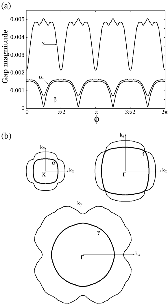
Figure 2: Calculated superconducting gap structure. (a) The gap magnitude on each of the three circular(cylindrical) Fermi surfaces, $\alpha$, $\beta$ and $\gamma$ is depicted as a function of the azimuthal angle $\phi$ around the $c$-axis (the Ru-O bonding direction corresponds to $\phi=0$). The unit of energy on the vertical axis is about 660(K). (b) The three Fermi surface sheets and the gap function. The Fermi surfaces are depicted by the thick solid lines. The dependence of the gap magnitude on in-plane direction is expressed by the distance from the Fermi circle along the direction.

The density of states (DOS) is calculated by the formula

$$\rho(\omega)=-\frac{1}{\pi}{\rm Im}\frac{1}{N}\sum_{a,\mib{k}}G_{a}^{\rm R}(\mib{k},\omega).$$ (65)

The density of states calculated for $T=0$ is shown in Fig. 3. The main part of the total DOS is taken by the main branch $\gamma$. The calculated partial DOS is 13.5 %, 29.1 % and 57.4 % of the total DOS for the $\alpha$, $\beta$ and $\gamma$ bands, respectively. This percentage is quantitatively consistent with the expectation from the de Haas-van Alphen measurement [38]. The main coherence peaks around $\omega=\pm 0.005$ are attributable to the DOS structure on the $\gamma$ band. The low energy part of the DOS near the Fermi level is dominated by the small-gap bands $\alpha$ and $\beta$. Our numerical result predicts that there are some fine structures between the main coherence peaks, which will originate from the coherence peaks on the $\alpha$ and $\beta$ bands. Actually, any spectroscopic measurements cannot detect such fine peak structures, due to their insufficient resolution. However, some inflection points might be observed in $\rho(\omega)$ as a function of energy $\omega$ by spectroscopies. Such fine structures, if they are indeed observed experimentally, could be considered as the nature of the orbital-dependent superconductivity [17].

Figure 3: Calculated density of states in the superconducting state. The vertical axis represents the density of states (arb. units) and the horizontal axis represents the energy $\omega$ (the Fermi level corresponds to $\omega=0$). The thick solid line denotes the total density of states, and the thin solid lines denote the contributions from each band. The unit of energy on the horizontal axis is about 660(K).

3.2 Analysis of ultrasound attenuation rate

Ultrasound attenuation rate is calculated by using the formula (53). The electron-phonon coupling matrix $\Lambda_{\mib{k},\mib{q},\ell\ell^{\prime}}$ is calculated by using eqs. (43)-(46). The constants $\tilde{g}_{i}$’s are determined by fitting to the experimental results of ref. References. In the present study we take $\tilde{g}_{1}=0.192$, $\tilde{g}_{2}=0.0096$, $\tilde{g}_{3}=0.0672$, $\tilde{g}_{4}=0.048$ and $\tilde{g}_{5}=0.03072$ for $\omega_{0}(\mib{q})=1.0$. The numerical results of ultrasound attenuation rate for various propagation and polarization directions are shown in Fig. 4. The remarkably strong anisotropy is in semiquantitative agreement with the experimental results (to be compared with Fig. 2 of ref. References). The attenuation rate of the sound mode L100 is about one thousand times larger than that of the mode T100. As pointed out by Walker and collaborators [34], this strong anisotropy is attributable to the anisotropy of electron-phonon interaction.

Figure 4: Calculated ultrasound attenuation rate for various sound propagation and polarization directions: (a) the longitudinal mode propagating along [100] direction and the transverse mode along [110] direction (i.e., L100: $\hat{\mib{e}}//\hat{\mib{q}}$, $\hat{\mib{q}}//[100]$, and T110: $\hat{\mib{e}}\perp\hat{\mib{q}}$, $\hat{\mib{q}}//[110]$), (b) the longitudinal mode along [110] direction (i.e., L110: $\hat{\mib{e}}//\hat{\mib{q}}$, $\hat{\mib{q}}//[110]$), and (c) the transverse mode along [100] direction (i.e., T100: $\hat{\mib{e}}\perp\hat{\mib{q}}$, $\hat{\mib{q}}//[100]$). This figure is to be compared with Fig. 2 in ref. References.

In Fig. 5, the numerical data are compared with the experimental data. In addition, the contributions from each band are separately presented there (note that the quantity is separable into the contributions from each band, since the formula (53) contains the summation with respect to band index $a$).

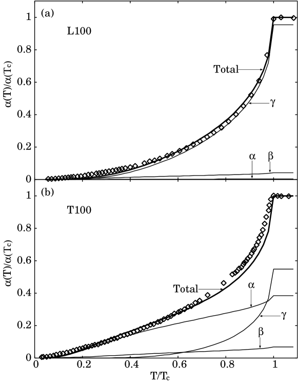
Figure 5: Calculated ultrasound attenuation rates (thick solid lines) are compared with the experimental data ($\diamond$) read from ref. References. (a) For the longitudinal wave propagating along [100] direction. (b) For the transverse wave propagating along [100] direction. The vertical and horizontal axes represent $\alpha(T)$ and temperature $T$ normalized by the value at $T=T_{\rm c}$, respectively. The contributions from each band are separately shown by the thin solid lines.

The numerical results are well fitted to the experimental results in the overall temperature region. For L100 mode we can see that the ultrasound attenuation is dominated by that on the $\gamma$ band. In this case the contributions from the $\alpha$ and $\beta$ bands are almost negligible. On the other hand, for T100 mode, the sound attenuation on the $\gamma$ band is ineffective, and the contribution from the $\gamma$ band is comparable to those from the $\alpha$ and $\beta$ bands. The attenuation at low temperatures is dominated by the passive bands, particularly the $\alpha$ band.

3.3 Analysis of thermal conductivity

The thermal conductivity along [100] direction (the directions of the thermal current and the temperature gradient are both along the $a$-axis) is calculated using the formula (64). After the fitting procedure for specific heat [23], there remains no fitting parameter, in contrast to the case of sound attenuation rate. The numerical results are shown in Fig. 6. There we can show also the contributions from each band separately (note that the quantity is separable into contributions from each band, since the formula (64) contains the summation with respect to band index $a$).

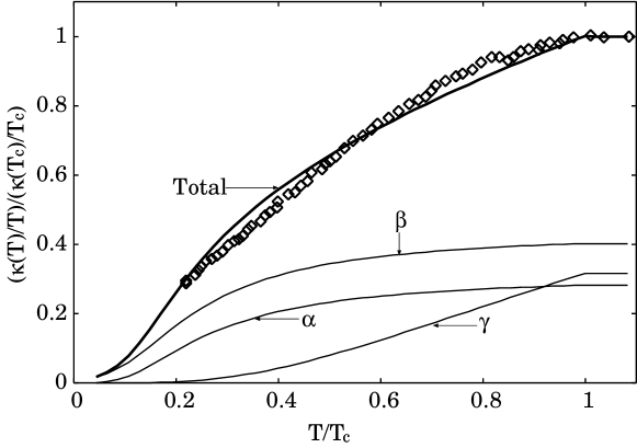
Figure 6: Calculated thermal conductivity $\kappa_{[100]}(T)$ (thick solid line) is compared with the experimental data ($\diamond$) read from ref. References. The vertical and horizontal axes represent $\kappa_{[100]}(T)/T$ and temperature $T$ normalized by the value at $T=T_{\rm c}$, respectively. The contributions from each band are separately shown by the thin solid lines.

It is very interesting that actually the passive bands $\alpha$ and $\beta$ contribute significantly to the thermal transport. Their contributions are comparable to that from the main branch $\gamma$. This situation is in contrast to other physical quantities in Sr₂RuO₄. For example, the main contribution to the specific heat is from the main branch $\gamma$ [23], since the $\gamma$ branch takes the main part of the total density of states. The reason why the main branch $\gamma$ is not dominant in the thermal transport is as follows. The superconducting gap on the main branch $\gamma$ has a node-like structure near the zone boundaries $(\pm\pi,0)$ and $(0,\pm\pi)$. However, the Fermi velocity $\mib{v}_{\mib{k}_{\rm F}}$ around these points is quite small, and therefore the thermally excited quasi-particles around there can not play an essential role for the transport (note that the formula (64) contains multiplication of the Fermi velocity). This situation demonstrates that the thermal transport property is inappropriate for detecting the gap anisotropy on the $\gamma$ branch.

4 Discussion

In this section, we suggest some remarks from the present calculation.

As we have seen in § 3.1, the gap structure is highly anisotropic. Although we have assumed naturally that the chiral state $\Delta(\mib{k})\sim k_{x}\pm{\rm i}k_{y}$ is realized, the gap function possesses sharp depressions on the $\beta$ Fermi surface (Fig. 2). This anisotropy is sufficiently large for explaining the power-law temperature dependence of various physical quantities. We obtain a good fitting for specific heat, using the present gap structure, as we have shown in the previous work [23]. We should note that this is a new mechanism of creating nodal gap structure. The incommensurate antiferromagnetic fluctuation actually causes the strong gap anisotropy on the $\alpha$ and $\beta$ bands. Our microscopic theory suggests the following rule generally: singlet[triplet] superconducting gap function should change[not change] its sign between the Fermi surface portions which are bridged by antiferromagnetic nesting vector, otherwise should take small values (i.e., nodal structure) on these Fermi surface portions. Recently, Kontani has applied the same scenario to nickel-borocarbide superconductors [50], which are considered to be a $s$-wave superconductor having a highly anisotropic gap. He considered the effect of antiferromagnetic spin fluctuation on $s$-wave superconducting gap structure, and showed that the gap magnitude is suppressed in the Fermi surface regions which the antiferromagnetic nesting vector bridges. These results suggest that nodal gap structure does not always originate from the symmetry properties of superconducting order parameter generally. So far, there have been a lot of phenomenological discussions. They have assumed that superconducting order parameter changes its sign on the nodes, and have discussed the symmetry properties of order parameter on the basis of the temperature dependence of physical quantities. Such phenomenology has often been applied to uranium heavy fermion superconductors [51]. However, as we have seen above, the validity of those phenomenological discussions is not so reliable in general.

Now we turn our attention to the specific discussions on the gap structure of Sr₂RuO₄. Recently Deguchi and Maeno measured specific heat under magnetic field [52, 53], in order to elucidate the detailed superconducting gap structure. They investigated the field-orientation dependence of specific heat. The anisotropy which is considered to originate from the gap anisotropy on the $\gamma$ band is observed to vanish at low temperatures. This might indicate the possibility that the small-gap bands ($\alpha$ and $\beta$) possess nodal structures near the diagonal lines, and the in-plane anisotropy from the active $\gamma$ band is canceled by that from the passive $\alpha$ and $\beta$ bands at low temperatures [53]. Recently Kusunose has analyzed the field-orientation dependence of $H_{c_{2}}$ and specific heat $C$ [54]. He showed that the gap structure with the intermediate magnitude of minima in $[100]$ direction for the $\gamma$ band, and tiny minima of gaps in $[110]$ directions for the $\alpha$ and $\beta$ bands give consistent behaviors with experiments. Particularly, he succeeded in explaining the anomalous temperature dependence of the in-plane anisotropy of $H_{c_{2}}$ [54], i.e., the sign change of $\delta H_{c_{2}}$ near $T_{\rm c}$ [55]. These experimental and theoretical results are consistent with our gap structure. Further investigations should be performed toward the thorough clarification of the gap structure of Sr₂RuO₄.

We have used the electron-phonon coupling constants $\tilde{g}_{i}$’s as fitting parameters. It is very difficult to determine these parameters microscopically without the fitting. In order to determine the parameters $\tilde{g}_{i}$’s without the fitting, it will be indispensable to know microscopically how the atoms are rearranged in order to relax the local stress (or strain), because $\tilde{g}_{i}$’s will essentially depend on the way of the rearrangement. For example, the stress along $[100]$ direction can be relaxed by reducing the Ru-O-Ru angle from 180 degrees without shrinking the Ru-O bonds along [100] direction, as well as by shrinking Ru-O bonds without changing the Ru-O-Ru angle. $\tilde{g}_{i}$’s will be different between these two ways of relaxation.

We have found actually that the overall temperature dependence and anisotropy of the ultrasound attenuation rate depend significantly on the parameters $\tilde{g}_{i}$’s. For example, we have shown the results in which $\alpha(T)/\alpha(T_{\rm c})$ for L100 is smaller than that for T100 (Compare Fig. 5(a) with Fig. 5(b)). However, we can actually show by using other parameter sets of $\tilde{g}_{i}$’s that $\alpha(T)/\alpha(T_{\rm c})$ for L100 could be larger than that for T100. Therefore it is actually difficult to determine the superconducting gap anisotropy by the experimental data of ultrasound attenuation rate without any detailed information on the electron-phonon coupling matrix elements.

We find still slight deviation between the theoretical and experimental results of ultrasound attenuation rate in Fig. 5, particularly at low temperatures in Fig. 5(a). We could consider various reasons for the deviation. One possible reason is that we could not reproduce the Fermi surface deformation precisely by using only five components of the electron-phonon coupling matrix elements. To obtain better agreement, we might require higher order harmonics of the matrix elements.

Recently Contreras et al. have obtained a good fitting of the ultrasound attenuation rate in Sr₂RuO₄ [30]. Note that their gap structure is quite different from ours. They claim that point nodes should be located on the $\gamma$ and $\beta$ bands [30]. However, it might be difficult to reproduce the line-node-like behaviors observed experimentally in many quantities. In addition, since the jump of specific heat at $T_{\rm c}$ will be larger than that in the line-node case, it is unclear whether or not to obtain consistency with the experiment of specific heat. From our microscopic point of view, we expect that, since the pairing interaction could possess only negligible momentum dependence along the $c$-axis due to the strong two-dimensionality, point nodes as well as horizontal line nodes are almost impossible to realize in Sr₂RuO₄.

The field-orientation dependence of thermal conductivity has been utilized to investigate the anisotropy of superconducting gap [15, 16, 56]. Izawa et al. observed actually negligible in-plane fourfold-symmetry component in the field-orientation dependence of the thermal conductivity, and concluded that line node should run around the cylindrical Fermi surfaces (horizontal line node) [15]. As we have shown in the present work, thermal conductivity is ineffective for detecting the gap anisotropy on the $\gamma$ band. This will be the reason why the gap anisotropy of the $\gamma$ band can be observed in field-oriented specific heat [52, 53], but not in field-oriented thermal conductivity [15, 56]. Therefore one might expect that thermal conductivity is appropriate for detecting the gap anisotropy on the passive bands $\alpha$ and $\beta$. However the fourfold-symmetry component of the field-orientated thermal conductivity may barely be detectable for the $\alpha$ and $\beta$ bands, as Tanaka et al. demonstrated [27]. We consider that the field-oriented thermal conductivity does not crucially exclude the possibility of line nodes along the $c$-axis.

In any case, we could conclude that line-node-like structure should exist on the $\alpha$ or $\beta$ band, by combining the following two points: (1) the $T$-linear behavior of $\kappa/T$ indicates that line-node-like structure should exist somewhere on the Fermi surface and (2) the thermal excitation on the $\gamma$ band does not effectively contribute to the thermal transport. However, it would still be difficult to obtain some insights into the nodal position only from the present analysis of thermal conductivity.

Recently Yanase et al. proposed another type of gap structure [57]. Although the essence of their pairing mechanism is the same as ours [58], the gap structure is a little different from ours: the nodal position on the $\beta$ band deviates from the diagonals. It is still controversial whether such a deviation is realized or not.

For determining the nodal positions thoroughly, it would be required to measure the gap magnitude by some momentum-resolving experiment on the Fermi surface. Further experimental probes crucially determining the nodal positions are desired to be developed.

5 Conclusion

In the present article, we have discussed the transport properties in the superconducting state of Sr₂RuO₄, by analyzing the sound attenuation rate and thermal conductivity. We have shown that the gap structure given in Fig. 2 is consistent with the experimental data.

As we have seen in Fig. 2, we obtain a nodal gap structure with a large in-plane anisotropy, particularly on the passive bands $\alpha$ and $\beta$, even if we assume the chiral state $\Delta(\mib{k})\sim k_{x}\pm{\rm i}k_{y}$. We should note this is a new mechanism of creating nodal gap structure: antiferromagnetic fluctuation deforms the gap structure, and creates the nodal gap structure. We do not consider that such a nodal structure due to this mechanism occurs exceptionally only in Sr₂RuO₄. We consider that a nodal structure could occur due to this mechanism also in other superconductors, particularly likely in strongly correlated electron systems. Therefore we should notice generally: actually it is not reliable to determine pairing symmetry by power-law temperature dependence of physical quantities.

Through the present study, we would like to stress that too much simplified models (e.g., an isotropic Fermi surface, only a single band or a gap function approximated by only a few harmonic functions.) are insufficient in general to analyze the anisotropy and the temperature dependence of physical quantities. In addition, we should note in general that some quantities can succeed in detecting the anisotropy of superconducting gap, but others can not. An example is the thermal conductivity in Sr₂RuO₄, which would fail to detect the in-plane gap anisotropy on the $\gamma$ band, as we have discussed in § 4.

In any case, we consider that it is very difficult to explain the experimental data without assuming the existence of line nodes on the passive small-gap bands $\alpha$ and $\beta$.

The present work is one of a few examples in which physical quantities are analyzed with use of realistic many-band electronic structure and superconducting gap structure obtained by microscopic calculation. In conclusion, we hope that such detailed analyses are performed also for many other anisotropic superconductors.

Appendix A Electron-Phonon Coupling Matrix

We consider the electron-phonon interaction, since the change of electronic structure due to lattice distortion is essential for the ultrasound attenuation. The detailed information about the anisotropy of electron-phonon interaction is actually important for the realistic analysis, as Walker et al. pointed out [34].

The non-interacting part of the Hamiltonian $H_{0}$ is written in the form,

$$H_{0}=\sum_{ii^{\prime},\ell\ell^{\prime},\sigma}t_{\ell\ell^{\prime}}[\mib{r}_{i}-\mib{r}_{i^{\prime}}]c_{i\ell\sigma}^{{\dagger}}c_{i^{\prime}\ell^{\prime}\sigma}.$$ (66)

$t_{\ell\ell^{\prime}}[\mib{r}_{i}-\mib{r}_{i^{\prime}}]$ is the transfer matrix element between the Wannier atomic orbitals $\ell$ at $i$-th site and $\ell^{\prime}$ at $i^{\prime}$-th site . Now the lattice deformation is introduced:

$$H_{0}=\sum_{ii^{\prime},\ell\ell^{\prime},\sigma}t_{\ell\ell^{\prime}}[(\mib{r}_{i}+\mib{u}_{i})-(\mib{r}_{i^{\prime}}+\mib{u}_{i^{\prime}})]c_{i\ell\sigma}^{{\dagger}}c_{i^{\prime}\ell^{\prime}\sigma}.$$ (67)

$\mib{u}_{i}$ is the displacement of the $i$-th Ru atom. The hopping integrals are expanded in $\mib{u}_{i}$:

$$t_{\ell\ell^{\prime}}[(\mib{r}_{i}+\mib{u}_{i})-(\mib{r}_{i^{\prime}}+\mib{u}_{i^{\prime}})]$$

$$=t_{\ell\ell^{\prime}}[\mib{r}_{i}-\mib{r}_{i^{\prime}}]+\mib{g}_{\ell\ell^{\prime}}(\mib{r}_{i}-\mib{r}_{i^{\prime}})\cdot(\mib{u}_{i}-\mib{u}_{i^{\prime}})+...,$$ (68)

where $\mib{g}_{\ell\ell^{\prime}}(\mib{r}_{i}-\mib{r}_{i^{\prime}})=\partial t_{\ell\ell^{\prime}}[\mib{a}]/\partial\mib{a}|_{\mib{a}=\mib{r}_{i}-\mib{r}_{i^{\prime}}}$ The Hamiltonian of the electron-phonon interaction is given by

$$H_{\rm ep}=\sum_{ii^{\prime},\ell\ell^{\prime},\sigma}\mib{g}_{\ell\ell^{\prime}}(\mib{r}_{i}-\mib{r}_{i^{\prime}})\cdot(\mib{u}_{i}-\mib{u}_{i^{\prime}})c_{i\ell\sigma}^{{\dagger}}c_{i^{\prime}\ell^{\prime}\sigma}.$$ (69)

Then we transform the expression to the momentum representation, and apply the second quantization to the lattice vibration,

$$H_{\rm ep}=\sum_{\mib{R},\ell\ell^{\prime},\sigma}(\mib{g}_{\ell\ell^{\prime}}(\mib{R})\cdot\hat{\mib{e}})\sum_{\mib{q}}(2NM{\omega}_{0}(\mib{q}))^{-1/2}$$

$$\times\sum_{\mib{k}}e^{-{\rm i}\mib{k}\cdot\mib{R}}(1-e^{-{\rm i}\mib{q}\cdot\mib{R}})(b_{\mib{q}}+b_{-\mib{q}}^{{\dagger}})c_{\mib{k}+\mib{q}\ell\sigma}^{{\dagger}}c_{\mib{k}\ell^{\prime}\sigma}.$$ (70)

Thus the Hamiltonian takes the form of eq. (42), using the electron-phonon coupling matrix

$$\Lambda_{\mib{k},\mib{q},\ell\ell^{\prime}} \equiv (2M{\omega}_{0}(\mib{q}))^{-1/2}\sum_{\mib{R}}e^{-{\rm i}\mib{k}\cdot\mib{R}}$$ (71)

$$\times(\mib{g}_{\ell\ell^{\prime}}(\mib{R})\cdot\hat{\mib{e}})(1-e^{-{\rm i}\mib{q}\cdot\mib{R}}).$$

$M$ is the ionic mass, $\omega_{\mib{q}}$ is the phonon frequency, and $b_{\mib{q}}$($b_{\mib{q}}^{{\dagger}}$) is the annihilation(creation) operator of the phonon with momentum $\mib{q}$ and polarization $\hat{\mib{e}}$. The unit vector $\hat{\mib{e}}$ points to the phonon polarization direction. In the actual experiment, the phonon wavenumber is much larger than the lattice constant ($\mib{q}\ll 1$), while the summation in $\mib{R}$ of eq. (70) is performed at most up to the second nearest sites. Therefore, $H_{\rm ep}$ is approximated as follows by expanding the factor $e^{-{\rm i}\mib{q}\cdot\mib{R}}$ in the power of $\mib{q}$ and neglecting higher orders:

$$\Lambda_{\mib{k},\mib{q},\ell\ell^{\prime}}={\rm i}(2M{\omega}_{0}(\mib{q}))^{-1/2}\sum_{\mib{R}}e^{-{\rm i}\mib{k}\cdot\mib{R}}(\mib{g}_{\ell\ell^{\prime}}(\mib{R})\cdot\hat{\mib{e}})(\mib{q}\cdot\mib{R}).$$ (72)

Here we consider the specific expression of the function $\mib{g}_{\ell\ell^{\prime}}(\mib{R})$. Since we expect naturally that the electronic transfers perpendicular to the direction of the deformation are not significantly affected by the deformation, we may assume that $\mib{g}_{\ell\ell^{\prime}}(\mib{R})$ is parallel to the vector $\mib{R}$:

$$\mib{g}_{\ell\ell^{\prime}}(\mib{R})=g_{\ell\ell^{\prime}}(\mib{R})\hat{\mib{R}}.$$ (73)

$\hat{\mib{R}}$ is the unit vector along $\mib{R}$, i.e., $\hat{\mib{R}}=\mib{R}/|\mib{R}|$, and $g_{\ell\ell^{\prime}}(\mib{R})$ is an even function of $\mib{R}$ [i.e., $g_{\ell\ell^{\prime}}(\mib{R})=g_{\ell\ell^{\prime}}(-\mib{R})$]. The coefficients $g_{\ell\ell^{\prime}}(\mib{R})$ are characterized by five constants, since we have taken the five hopping integrals ($t_{1},...,t_{5}$) for describing the electronic structure:

$$g_{xy,xy}(\hat{\mib{x}}) = g_{1},$$ (74)

$$g_{xz,xz}(\hat{\mib{x}}) = g_{3},$$ (75)

$$g_{yz,yz}(\hat{\mib{x}}) = g_{4},$$ (76)

$$g_{xy,xy}(\hat{\mib{y}}) = g_{1},$$ (77)

$$g_{xz,xz}(\hat{\mib{y}}) = g_{4},$$ (78)

$$g_{yz,yz}(\hat{\mib{y}}) = g_{3},$$ (79)

$$g_{xy,xy}(\hat{\mib{x}}+\hat{\mib{y}}) = g_{2},$$ (80)

$$g_{yz,xz}(\hat{\mib{x}}+\hat{\mib{y}}), = g_{xz,yz}(\hat{\mib{x}}+\hat{\mib{y}})=g_{5},$$ (81)

$$g_{xy,xy}(\hat{\mib{x}}-\hat{\mib{y}}) = g_{2},$$ (82)

$$g_{yz,xz}(\hat{\mib{x}}-\hat{\mib{y}}) = g_{xz,yz}(\hat{\mib{x}}-\hat{\mib{y}})=-g_{5},$$ (83)

and the other elements of $g_{\ell\ell^{\prime}}(\mib{R})$ are zero, where $\hat{\mib{x}}$($\hat{\mib{y}}$) is the unit lattice vector along the $x$-($y$-)axis. We obtain the momentum-dependent electron-phonon coupling matrix elements in eqs. (43)-(46), by substituting eqs. (74)-(83) into eq. (72) and using the coefficients $\tilde{g}_{i}$’s related to $g_{i}$’s as $\tilde{g}_{1}=2\gamma g_{1}$, $\tilde{g}_{2}=2^{3/2}\gamma g_{2}$, $\tilde{g}_{3}=2\gamma g_{3}$, $\tilde{g}_{4}=2\gamma g_{4}$, $\tilde{g}_{5}=2^{3/2}\gamma g_{5}$ ($\gamma=\{\omega_{0}(\mib{q})/(2Mv_{\mib{q}}^{2})\}^{1/2}$, and $v_{\mib{q}}$ is the sound velocity).

Appendix B Charge Neutrality Condition under Lattice Deformation

In this Appendix, we consider the local charge neutrality condition, which should be retained under the lattice distortion due to the ultrasound propagation. We introduce a lattice distortion described by $\eta\phi_{\mib{q}}$ [For the definition of $\phi_{\mib{q}}$, see eq. (42)], whose spatial periodicity is characterized by the wavenumber $\mib{q}$. $\eta$ is related to the magnitude of the displacement of the atoms. This distortion plays a role of periodic potential acting on the electron system. The electron self-energy will be modified by

$$\Sigma_{\ell\ell^{\prime}}(\mib{k};q)=\eta D(q)\Lambda_{\mib{k},\mib{q},\ell\ell^{\prime}}.$$ (84)

Figure 7: The diagrammatic representation of the lowest-order electron self-energy correction due to the lattice distortion $\eta\phi_{\mib{q}}$.

Now we focus on a local small volume, which is enough smaller than the characteristic length of lattice distortion ($\sim 2\pi/|\mib{q}|$) but still contains macroscopic number of electrons. In this volume, the electron system is regarded as spatially uniform. As far as we discuss the properties of the electrons contained in this small volume, we can use the Green’s function $G_{\ell\ell^{\prime}}(k)$ corrected by the self-energy $\Sigma_{\ell\ell^{\prime}}(\mib{k};q)$. The local change of electron number is obtained by

$$\delta n = 2\frac{T}{N}\sum_{k,\ell}[G_{\ell\ell}(k)-G_{\ell\ell}^{(0)}(k)]$$ (85)

$$\approx 2\frac{T}{N}\sum_{a,k}\frac{\partial G^{(0)}_{a}(k)}{\partial\xi_{a}(\mib{k})}$$

$$\times\sum_{\ell_{1}\ell_{2}}U_{a\ell_{1}}^{{\dagger}}(\mib{k})U_{\ell_{2}a}(\mib{k})\Sigma_{\ell_{1}\ell_{2}}(\mib{k};q),$$

within the precision to the lowest order in $\eta$, and we have used similar relations to eqs. (23) and (24). The charge neutrality condition states that the charge inhomogeneity caused by the lattice distortion $\eta\phi_{\mib{q}}$ should be canceled by introducing a local change of electron chemical potential [41]:

$$\frac{1}{N}\sum_{a,\mib{k}}(\partial_{\xi}G)_{a}(\mib{k})\biggl{[}\sum_{\ell_{1}\ell_{2}}U_{a\ell_{1}}^{{\dagger}}(\mib{k})U_{\ell_{2}a}(\mib{k})\Sigma_{\ell_{1}\ell_{2}}(\mib{k};q)$$

$$-\Delta\mu\biggr{]}\approx 0,$$ (86)

where $(\partial_{\xi}G)_{a}(\mib{k})$ is defined as

$$(\partial_{\xi}G)_{a}(\mib{k})\equiv T\sum_{\omega_{n}}\frac{\partial G_{a}^{(0)}(k)}{\partial\xi_{a}(\mib{k})}.$$ (87)

We obtain from eq. (86)

$$\Delta\mu=\frac{\sum_{a,\mib{k},\ell_{1}\ell_{2}}\{(\partial_{\xi}G)_{a}(\mib{k})\}U_{a\ell_{1}}^{{\dagger}}(\mib{k})U_{\ell_{2}a}(\mib{k})\Sigma_{\ell_{1}\ell_{2}}(\mib{k};q)}{\sum_{a,\mib{k}}(\partial_{\xi}G)_{a}(\mib{k})}.$$ (88)

Here let us note that the shift of chemical potential $\Delta\mu$ can be regarded as a renormalization of the electron-phonon coupling matrix elements $\Lambda_{\mib{k},\mib{q},\ell\ell^{\prime}}$. The chemical potential shift $\Delta\mu$ appears in the equations always together with the self-energy in the form, $\Sigma_{\ell\ell^{\prime}}(\mib{k};q)-\Delta\mu\delta_{\ell\ell^{\prime}}$. If we define the mean value of $\Lambda_{\mib{k},\mib{q},\ell\ell^{\prime}}$ by eq. (LABEL:eq:LambdaMeanValue), then

$$\Sigma_{\ell\ell^{\prime}}(\mib{k};q)-\Delta\mu\delta_{\ell\ell^{\prime}}=\eta D(q)(\Lambda_{\mib{k},\mib{q},\ell\ell^{\prime}}-\bar{\Lambda}_{\mib{q}}\delta_{\ell\ell^{\prime}}).$$ (89)

Thus the local charge neutrality condition is satisfied by using the renormalized value of the electron-phonon coupling, $\Lambda_{\mib{k},\mib{q},\ell\ell^{\prime}}-\bar{\Lambda}_{\mib{q}}\delta_{\ell\ell^{\prime}}$, instead of $\Lambda_{\mib{k},\mib{q},\ell\ell^{\prime}}$.

In the normal state, using eqs. (11) and (87), we obtain

$$(\partial_{\xi}G)_{a}(\mib{k})=-\frac{\partial n_{\rm F}(\epsilon)}{\partial\epsilon}\biggr{|}_{\epsilon=\xi_{a}(\mib{k})}.$$ (90)

$n_{\rm F}(\epsilon)$ is the Fermi function. In the superconducting state, we obtain eq. (57) by using eq. (87) and $G_{a}^{(0)}(k)$ of the form

$$G_{a}^{(0)}(k)=-\frac{{\rm i}\omega_{n}+\xi_{a}(\mib{k})}{\omega_{n}^{2}+{\xi_{a}(\mib{k})}^{2}+|\Delta_{a}(\mib{k})|^{2}}.$$ (91)

Appendix C About the Strong Gap Anisotropy on the $\alpha$ and $\beta$ Bands

In this Appendix, we discuss the origin of the strong gap anisotropy on the $\alpha$ and $\beta$ bands by extracting the pairing interaction $V_{a\sigma_{1}\sigma_{2},a^{\prime}\sigma_{3}\sigma_{4}}(k,k^{\prime})$ in eq. (12). We focus on the values of $V_{\beta\sigma\sigma,\beta\sigma\sigma}(k,k^{\prime})$ and $V_{\beta\sigma\sigma,\alpha\sigma\sigma}(k,k^{\prime})$ on the Fermi surface. We characterize position on the Fermi surface by the in-plane azimuthal angle $\phi$ with respect to the Ru-O bonding direction. Hereafter we refer to the values of $V_{\beta\sigma\sigma,\beta\sigma\sigma}(k,k^{\prime})$ and $V_{\beta\sigma\sigma,\alpha\sigma\sigma}(k,k^{\prime})$ on the Fermi surface as $V_{\beta,\beta}(\phi_{\beta};\phi^{\prime}_{\beta})$ and $V_{\beta,\alpha}(\phi_{\beta};\phi^{\prime}_{\alpha})$, respectively (The Matsubara frequencies $\omega_{n}$ and $\omega^{\prime}_{n}$ are fixed to $\pi T$). Now we fix the initial state of Cooper pair on the $\beta$ Fermi surface by $\phi_{\beta}=\frac{\pi}{4}$ as pointed in Fig. 8(a). $V_{\beta,\beta}(\phi_{\beta}=\pi/4;\phi^{\prime}_{\beta})$ and $V_{\beta,\alpha}(\phi_{\beta}=\pi/4;\phi^{\prime}_{\alpha})$ are depicted as a function of the angles $\phi^{\prime}_{\beta}$ and $\phi^{\prime}_{\alpha}$, respectively, in Fig. 8(b). We find that there are characteristic local minimum in $V_{\beta,\beta}(\phi_{\beta}=\pi/4;\phi^{\prime}_{\beta})$ around $\phi^{\prime}_{\beta}=5\pi/4$ and local maximum in $V_{\beta,\alpha}(\phi_{\beta}=\pi/4;\phi^{\prime}_{\alpha})$ around $\phi^{\prime}_{\alpha}=\pi/4$. The local minimum of $V_{\beta,\beta}(\phi_{\beta}=\pi/4;\phi^{\prime}_{\beta})$ around $\phi^{\prime}_{\beta}=5\pi/4$ favors the same sign of order parameter between the points $\phi_{\beta}=\pi/4$ and $\phi^{\prime}_{\beta}=5\pi/4$. The local maximum of $V_{\beta,\alpha}(\phi_{\beta}=\pi/4;\phi^{\prime}_{\alpha})$ around $\phi^{\prime}_{\alpha}=\pi/4$ favors the different sign of order parameter between the points $\phi_{\beta}=\pi/4$ and $\phi^{\prime}_{\alpha}=\pi/4$. These momentum dependences deform the gap structure on the $\alpha$ and $\beta$ bands significantly, and result in the strong anisotropy of gap structure. Those characteristic momentum dependences of the pairing interaction basically originate from those of the fluctuation due to the nesting between the $\alpha$ and $\beta$ Fermi surfaces, although it is somewhat modulated by the diagonalization matrix $U(\mib{k})$ in eq. (10).

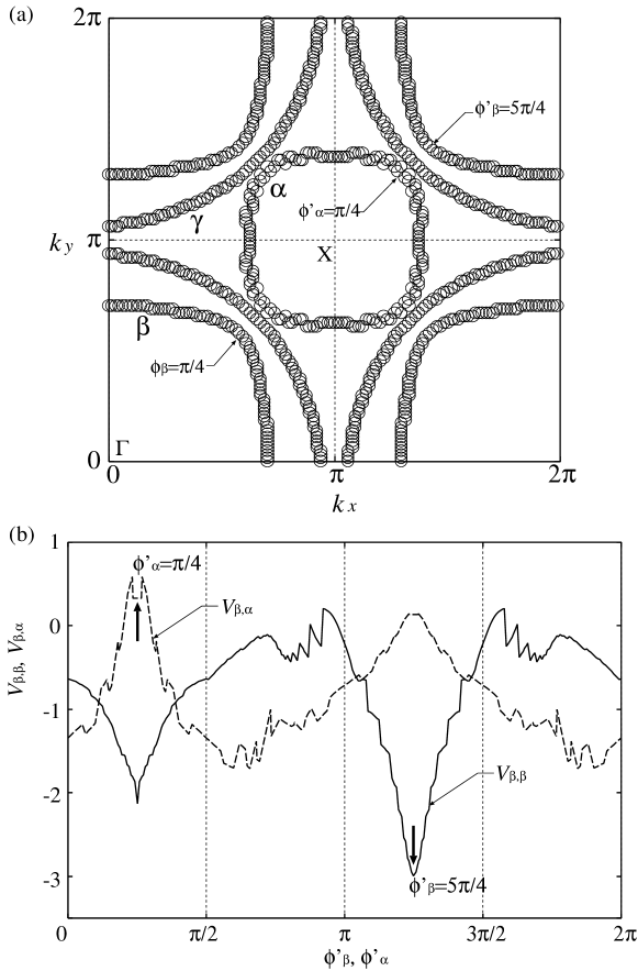
Figure 8: (a) The three Fermi surfaces, $\alpha$, $\beta$ and $\gamma$ are depicted. Position on the Fermi surfaces $\beta$[$\alpha$] is characterized by the in-plane azimuthal angle $\phi$ around the points $\Gamma(0,0)$[$X(\pi,\pi)$] with respect to the $x$-axis. (b) Calculated effective pair-scattering amplitudes $V_{\beta,\beta}(\phi_{\beta}=\pi/4;\phi^{\prime}_{\beta})$ and $V_{\beta,\alpha}(\phi_{\beta}=\pi/4;\phi^{\prime}_{\alpha})$ are shown as a function of the azimuthal angles $\phi^{\prime}_{\beta}$ and $\phi^{\prime}_{\alpha}$, respectively.

References

• [1] For a review, A.P. Mackenzie and Y. Maeno: Rev. Mod. Phys. 75 (2003) 657.
• [2] K. Ishida, H. Mukuda, Y. Kitaoka, K. Asayama, Z.Q. Mao, Y. Mori and Y. Maeno: Nature 396 (1998) 658.
• [3] J. A. Duffy, S. M. Hayden, Y. Maeno, Z. Mao, J. Kulda and G. J. McIntyre: Phys. Rev. Lett. 85 (2000) 5412.
• [4] T.M. Rice and M. Sigrist: J. Phys.: Condens. Matter 7 (1995) L643.
• [5] I.I. Mazin and D.J. Singh: Phys. Rev. Lett. 79 (1997) 733.
• [6] Y. Sidis, M. Braden, P. Bourges, B. Hennion, S. NishiZaki, Y. Maeno and Y. Mori: Phys. Rev. Lett. 83 (1999) 3320.
• [7] T. Nomura and K. Yamada: J. Phys. Soc. Jpn. 69 (2000) 3678.
• [8] T. Nomura and K. Yamada: J. Phys. Soc. Jpn. 71 (2002) 1993.
• [9] Y. Yanase, T. Jujo, T. Nomura, H. Ikeda, T. Hotta and K. Yamada: Phys. Rep. 387 (2003) 1.
• [10] G.M. Luke, Y. Fudamoto, K.M. Kojima, M.I. Larkin, J. Merrin, B. Nachumi, Y.J. Uemura, Y. Maeno, Z.Q. Mao, Y. Mori, H. Nakamura and M. Sigrist: Nature 394 (1998) 558.
• [11] S. NishiZaki, Y. Maeno and Z.Q. Mao: J. Phys. Soc. Jpn. 69 (2000) 572.
• [12] K. Ishida, H. Mukuda, Y. Kitaoka, Z.Q. Mao, Y. Mori and Y. Maeno: Phys. Rev. Lett. 84 (2000) 5387.
• [13] I. Bonalde, B.D. Yanoff, M.B. Salamon, D.J. Van Harlingen, E.M.E. Chia, Z.Q. Mao and Y. Maeno: Phys. Rev. Lett. 85 (2000) 4775.
• [14] C. Lupien, W.A. MacFarlane, C. Proust, L. Taillefer, Z.Q. Mao and Y. Maeno: Phys. Rev. Lett. 86 (2001) 5986.
• [15] K. Izawa, H. Tanaka, H. Yamaguchi, Y. Matsuda, M. Suzuki, T. Sasaki, T. Fukase, Y. Yoshoda, R. Settai and Y. Onuki: Phys. Rev. Lett. 86 (2001) 2653.
• [16] M.A. Tanatar, S. Nagai, Z.Q. Mao, Y. Maeno and T. Ishiguro: Phys. Rev. B 63 (2001) 064505.
• [17] D.F. Agterberg, T.M. Rice and M. Sigrist: Phys. Rev. Lett. 78 (1997) 3374.
• [18] K. Miyake and O. Narikiyo: Phys. Rev. Lett. 83 (1999) 1423.
• [19] Y. Hasegawa, K. Machida and M. Ozaki: J. Phys. Soc. Jpn. 69 (2000) 336.
• [20] H. Won and K. Maki: Europhys. Lett. 52 (2000) 427.
• [21] T. Dahm, H. Won and K. Maki: cond-mat/0006301.
• [22] M.E. Zhitomirsky and T.M. Rice: Phys. Rev. Lett. 87 (2001) 057001.
• [23] T. Nomura and K. Yamada: J. Phys. Soc. Jpn. 71 (2002) 404.
• [24] J. Moreno and P. Coleman: Phys. Rev. B 53 (1996) R2995.
• [25] M.J. Graf and A.V. Baratsky: Phys. Rev. B 62 (2000) 9697.
• [26] W.C. Wu and R. Joynt: Phys. Rev. B 64 (2001) 100507.
• [27] Y. Tanaka, K. Kuroki, Y. Tanuma and S. Kashiwaya: J. Phys. Soc. Jpn. 72 (2003) 2157.
• [28] H. Kusunose and M. Sigrist: Europhys. Lett.60 (2002) 281.
• [29] M. Udagawa, Y. Yanase and M. Ogata: Phys. Rev. B 70 (2004) 184515.
• [30] P. Contreras, M. Walker and K. Samokhin: Phys. Rev. B 70 (2004) 184528.
• [31] P.J. Hirschfeld, D. Vollhardt and P. Wölfle: Solid State Commun. 59 (1986) 111.
• [32] S. Schmitt-Rink, K. Miyake and C.M. Varma: Phys. Rev. Lett. 57 (1986) 2575.
• [33] P.J. Hirschfeld, P. Wölfle and D. Einzel: Phys. Rev. B 37 (1988) 83.
• [34] M.B. Walker, M.F. Smith and K.V. Samokhin: Phys. Rev. B 65 (2001) 014517.
• [35] T. Oguchi: Phys. Rev. B 51 (1995) 1385.
• [36] D.J. Singh: Phys. Rev. B 52 (1995) 1358.
• [37] This value of $t_{5}$ is a little smaller than that in ref. References, for which the Fermi surfaces $\alpha$ and $\beta$ become more tetragonal than those in ref. References. Calculated specific heat fits to the experimental data as well as in ref. References.
• [38] A.P. Mackenzie, S.R. Julien, A.J. Diver, G.J. McMullan, M.P. Ray, G.G. Lonzarich, Y. Maeno, S. Nishizaki and T. Fujita: Phys. Rev. Lett. 76 (1996) 3786.
• [39] A. Damascelli, D.H. Lu, K.M. Shen, N.P. Armitage, F. Ronning, D.L. Feng, C. Kim, Z.X. Shen, T. Kimura, Y. Tokura, Z.Q. Mao and Y. Maeno: Phys. Rev. Lett. 85 (2000) 5194.
• [40] For a textbook, J. Rammer: Quantum Transport Theory (Westview Press; Perseus Books Group, U.S., 2004).
• [41] For a textbook, A.A. Abrikosov: Fundamentals of the Theory of Metals (Elsevier Science Publishers B.V., North-Holland, 1988).
• [42] For a textbook, V.P. Mineev and K.V. Samokhin: Introduction to Unconventional Superconductivity (Gordon and Breach Science Publishers, New York, 1999).
• [43] J.S. Langer: Phys. Rev. 128 (1962) 110.
• [44] J.M. Luttinger: Phys. Rev. 135 (1964) A1505.
• [45] I.I. Mazin and D.J. Singh: Phys. Rev. Lett. 82 (1999) 4324.
• [46] T. Nomura and K. Yamada: J. Phys. Soc. Jpn. 69 (2000) 1856.
• [47] I. Eremin, D. Manske and K.H. Bennemann: Phys. Rev. B 65 (2001) 220502.
• [48] N. Kikugawa, C. Bergemann, A.P. Mackenzie and Y. Maeno: Phys. Rev. B 70 (2004) 134520.
• [49] K. Kuroki, M. Ogata, R. Arita and H. Aoki: Phys. Rev. B 63 (2001) 060506.
• [50] H. Kontani: Phys. Rev. B 70 (2004) 054507.
• [51] K. Machida, T. Nishira and T. Ohmi: J. Phys. Soc. Jpn. 68 (1999) 3364.
• [52] K. Deguchi, Z.Q. Mao, H. Yaguchi and Y. Maeno: Phys. Rev. Lett. 92 (2004) 047002.
• [53] K. Deguchi, Z.Q. Mao and Y. Maeno: J. Phys. Soc. Jpn. 73 (2004) 1313.
• [54] H. Kusunose: J. Phys. Soc. Jpn. 73 (2004) 2512.
• [55] Z.Q. Mao, Y. Maeno, S. Nishizaki, T. Akima and T. Ishiguro: Phys. Rev. Lett. 84 (2000) 991.
• [56] M.A. Tanatar, M. Suzuki, S. Nagai, Z.Q. Mao, Y. Maeno and T. Ishiguro: Phys. Rev. Lett. 86 (2001) 2649.
• [57] Y. Yanase and M. Ogata: unpublished.
• [58] Y. Yanase and M. Ogata: J. Phys. Soc. Jpn. 72 (2003) 673.