Abstract

By a combination of analytical and numerical techniques, we analyze the continuum limit of the integrable $3\otimes\bar{3}\otimes 3\otimes\bar{3}\ldots$ $sl(2/1)$ superspin chain. We discover profoundly new features, including a continuous spectrum of conformal weights, whose numerical evidence is infinite degeneracies of the scaled gaps in the thermodynamic limit. This indicates that the corresponding conformal field theory has a non compact target space (even though our lattice model involves only finite dimensional representations). We argue that our results are compatible with this theory being the level $k=1$, ‘$SU(2/1)$ WZW model’ (whose precise definition requires some care). In doing so, we establish several new results for this model. With regard to potential applications to the spin quantum Hall effect, we conclude that the continuum limit of the $3\otimes\bar{3}\otimes 3\otimes\bar{3}\ldots$ $sl(2/1)$ integrable superspin chain is not the same as (and is in fact very different from) the continuum limit of the corresponding chain with two-superspin interactions only, which is known to be a model for the spin quantum Hall effect. The study of possible RG flows between the two theories is left for further study.

1 Introduction

The sigma model approach [1] to phase transitions in non interacting disordered systems provides a convenient and appealing description of the physics at hand. The best known example is the transition between plateaux in the integer quantum Hall effect (class A), which can be described using a $U(2n)/U(n)\times U(n)$ sigma model in the limit $n\rightarrow 0$. More recently, the equivalent ‘spin quantum Hall effect’ in d-wave superconductors has been considered (class C [2]), and described with the $SP(2n)/U(n)$ sigma model, in the limit $n\rightarrow 0$[3].

In both cases, the existence of a delocalization transition is associated with the masslessness in the IR of the sigma model at topological angle $\theta=\pi$. Identification of the corresponding conformal field theory would lead to a presumably exact determination of critical exponents which have been studied in great details in numerical works [4],[5] as well as in experiments.

Unfortunately, the determination of the IR fixed points in these problems has proven extremely difficult. The canonical example of what ‘might’ happen is the case $n=1$ of either replica model, which coincides with the $O(3)$ sigma model at $\theta=\pi$. In this case, there is a wealth of evidence [6] that the IR fixed point is the $SU(2)$ Wess Zumino model at level $k=1$. In the flow, the field is promoted from being coset valued to group valued, a highly non perturbative feature which might have been hard to believe, were it not for the existence of exact solutions [7].

The most reasonable way to understand what happens in the disordered system is first to trade the replica limit for a super group [8],[9], $U(1,1/2)/U(1/1)\times U(1/1)$ in the quantum Hall effect, and $OSP(2n/2n)/U(n|n)$ in the spin quantum Hall effect. Once the corresponding sigma models have been satisfactorily defined [10], it is then tempting to conjecture, by analogy with the $O(3)$ example above, what the IR fixed point might be. In this way, Zirnbauer [11] arrived at a proposal for the quantum Hall effect that is related with the WZW model (at level $k=1$) on $PSU(1,1/2)$. Roughly, this is obtained by observing that the base of the supersymmetric target space is $H^{2}\times S^{2}$, and then guessing that this gets ‘promoted’ to $H^{3}\times S^{3}$ in the IR. One then tries to build the minimal proposal in agreement with this and known results on the exponents. It is important that for the $PSU(1,1/2)$ WZW model the kinetic term is an exactly marginal deformation [12],[13]. The final proposal of Zirnbauer corresponds to a particular value of this kinetic term, and is not the WZW model. Hence, the symmetry is a global symmetry $G_{L}\times G_{R}$ instead of a local one. Unfortunately it is not clear whether this proposal gives the correct IR fixed point. In particular, it is rather unpleasant to have to select a particular value for an exactly marginal coupling constant if one hopes to describe what seems to be genuine universal physics.

A less abstract direction of attack comes from network models. These can be shown to correspond, in the proper anisotropic limit to quantum spin chains with super group symmetries [14]. Ideally, the problem would then be solved if one were able to apply in this situation the formidable arsenal developed over the years in the study of quantum spin chains. Unfortunately, there are difficulties here as well. For the ordinary as well as the spin quantum Hall effect, the Hilbert space of the chain is of type $V\otimes\bar{V}\otimes V\otimes\bar{V}\otimes\cdots$, while the Hamiltonian is the invariant Casimir, the proper generalization of $\vec{S}.\vec{S}$. In the ordinary quantum Hall effect, $V$ and $\bar{V}$ are infinite dimensional, while in the spin quantum Hall effect, $V$ and $\bar{V}$ are the two conjugate three dimensional representations.

In either case, the Hamiltonian is not integrable. More precisely, the Hamiltonian does not seem to derive from a family of commuting transfer matrices obtained via a standard quantum group approach. In the spin quantum Hall case, the Hamiltonian can however be diagonalized [15] (more precisely, the zeroes of the characteristic polynomial can be found, as the Hamiltonian itself is not fully diagonalizable) using known results about the XXZ chain and representation theory of the Temperley Lieb algebra [16]. No such approach seems possible in the ordinary quantum Hall spin chain.

Since one is after the universality class of the IR fixed point, it is natural to wonder [17] whether the Hamiltonian might be substituted by an integrable version without affecting the exponents. Examples are known where such a trick would not work: for instance, the higher odd spin integrable $SU(2)$ spin chains flow to level $k=2s$ WZW models, while the chains with Heisenberg type couplings flow to level $k=1$. But examples are also known where the trick does work. Indeed, with unitary groups and finite dimensional representations, group symmetry on the lattice plus criticality implies that the continuum limit is a WZW model, the stablest of all being $k=1$ [18]. Therefore, a spin chain with $SU(n)$ symmetry, if critical, will generically be in the same universality class as the integrable Sutherland chain, that is the level one $SU(n)$ WZW model. Criticality is however not guaranteed in general. For instance, if one takes $SU(n)$ and the alternance of $n$ and $\bar{n}$ representations, the chain whose Hamiltonian is the Casimir has a gap, while the integrable one is gapless, and in the universality class of the WZW model [19].

Our purpose in this paper is to explore the matter further by concentrating on the spin quantum Hall effect where many things are known exactly. In a nutshell, the question we want to explore is whether the integrable $3\otimes\bar{3}\otimes 3\otimes\bar{3}\ldots$ $sl(2/1)$ spin chain is massless and if so, in the same universality class as the non integrable$3\otimes\bar{3}\otimes 3\otimes\bar{3}\ldots$ Heisenberg chain, which is known to describe the physics of the spin quantum Hall effect.

A positive answer would raise hopes for an integrable approach to the ordinary quantum Hall effect. Unfortunately, we will see that the answer is a resounding no. The reason for this is the proliferation of possible fixed points that appear when ordinary compact symmetries are replaced by super group, maybe non compact, symmetries, and sheds light on what should be directions of further research.

We will present evidence from various sources that the integrable alternating $3,\bar{3}$ chain is in the universality class of the $SU(2/1)$ WZW model at level $1$[20]. This model has also been called $OSP(2/2)_{-2}$ in the literature [21], and has appeared previously in the study of Dirac fermions in a random gauge potential[22]. In contrast, it is already known from [16] that the non integrable alternating $3,\bar{3}$ Heisenberg chain does not scale to a WZW model, but to a new kind of theory, where the currents have logarithmic OPEs, and the symmetry is not of Kac Moody type [23].

It is important to stress here that the WZW model is a very different theory from the one [16] associated with the Heisenberg Hamiltonian; in particular, it has a continuous spectrum of critical exponents, which is not bounded from below. Trying to infer generic physical properties from the integrable chain would be a considerable mistake in this case, and presumably in the ordinary quantum Hall case as well.

The paper is organized as follows. In the next section, we gather information, obtained from the literature as well as our own calculations, about the WZW model. In sections three and four, we present the results of a numerical and analytical study of the Bethe ansatz equations of the integrable spin chain, comparing our results with the expectations for the WZW model. Section five contains elements of extension to the case of higher level. Section six goes back to the spin quantum Hall problem. Technical details are provided in the appendices.

2 First considerations on the WZW model

2.1 Algebraic generalities

We start with a short review of the “base” $sl(2/1)$ algebra. It contains a sub $sl(2)$ with generators $J^{\pm}_{0},J^{3}_{0}$, an extra $U(1)$ generator $B_{0}$, and two pairs of fermionic generators $V_{0}^{\pm}$ and $W_{0}^{\pm}$. Its representation theory is complicated, although this is one of the best understood cases in the super Lie algebra literature [24],[25],[26],[27]. Typical representations are characterized by a pair of numbers traditionally called $b,j$ (and denoted $[b,j]$ in what follows). Here, $j$ is a $sl(2)$ spin quantum number and takes values $0,1/2,1,\ldots$, whereas $b$ can be any complex number. Typicality requires $b\neq\pm j$. Typical representations are irreducible. Their dimension is $8j$, and they decompose into $sl(2)$ representations with spin $j,j-1/2,j-1/2,j-1$ with, respectively, $b$ numbers $b,b+1/2,b-1/2,b$ (for $j=1/2$, the value $j-1$ is omitted). We introduce the notation $\rho_{j}^{b}$ to denote an $sl(2)$ representation of spin $j$ for which the other $u(1)$ generator takes the constant value $b$, so the former decomposition reads $\rho_{j}^{b}\oplus\rho_{j-1/2}^{b+1/2}\oplus\rho_{j-1/2}^{b-1/2}\oplus\rho_{j-1}^{b}$. The Casimir is diagonal in these representations, and proportional to $j^{2}-b^{2}$.

A particularly important representation in the WZW model will be the four dimensional $[b=0,j=1/2]$ which is represented graphically in Fig. 1. It is the defining representation for $osp(2/2)$.

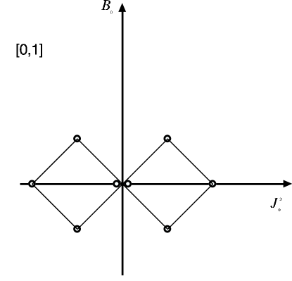
Figure 1: Graphical representation of the representation $[0,1/2]$.

There are many more representations. Simple atypical (that is, irreducible atypical) occur when $b=\pm j$, and have dimension $4j+1$. Examples are the three dimensional representations $[1/2,1/2]$ and $[-1/2,1/2]$ that we will use to define the ‘Hilbert’ space for the quantum spin chain. Representations $[j,j]$ contain only multiplets $\rho_{j}^{j}$ and $\rho_{j-1/2}^{j+1/2}$, so $[1/2,1/2]$ contains $\rho_{1/2}^{1/2}$ and $\rho_{0}^{1}$. Similarly, representations $[-j,j]$ contain only multiplets with $\rho_{j}^{-j}$ and $\rho_{j-1/2}^{j-1/2}$, so $[-1/2,1/2]$ contains $\rho_{1/2}^{-1/2}$ and $\rho_{0}^{-1}$. While typical representations have vanishing superdimension, simple atypical ones have superdimension equal to plus or minus one.

The other atypical representations are not simple: they are indecomposable but partly reducible, and form what is often called ‘blocks’. The most important example is the one appearing in the tensor product $[0,1/2]\otimes[0,1/2]$ which decomposes as the adjoint $[0,1]$ and another eight dimensional representation usually denoted as $[0,-1/2,1/2,0]$. This representation is the semi direct sum of $[1/2,1/2]$, $[-1/2,1/2]$, and of two $[0,0]$ representations. Its $su(2)$ content is $\rho_{1/2}^{1/2}$, $\rho_{1/2}^{-1/2}$ , $\rho_{0}^{1}$, $\rho_{0}^{-1}$, and $\rho_{0}^{0}$ twice. A graphical representation is given in figure 2. Note that this representation has vanishing superdimension.

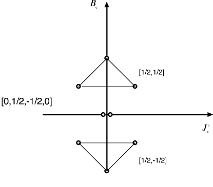
Figure 2: Graphical representation of the representation $[0,-1/2,1/2,0]$.

It is useful to represent such an indecomposable representation by its ‘quiver diagram’ [28]. Denote by $j$ the representation $[j,j]$ and by $-j$ the representation $[-j,j]$ (these simple atypical representations can be obtained by maximum supersymmetrization of the fundamental or its conjugate - $2j$ boxes in a Young diagram representation). Then the eight dimensional indecomposable can be represented as

$$\hbox{$\begin{array}[]{rcl}&{}^{0}_{\bullet}\\ \hphantom{-1}\swarrow&&\searrow\\ {}^{-1/2}_{~{}~{}\bullet}\hphantom{\swarrow}&&\hphantom{\swarrow}{}^{1/2}_{\bullet}\\ \makebox[0.0pt]{}\searrow&&\swarrow\\ &{}^{0}_{\bullet}\end{array}$}.$$ (2.1)

Here, the bottom part of the diagram means that the representation contains a singlet as an invariant subspace. There is then two submodules of dimension three which are not invariant but are (and then, isomorphic to $1/2$ and $-1/2$) modulo the singlet, and finally, on top, a submodule of dimension one which is invariant modulo all the others. A generic element of the algebra, written in the basis made of the top, middle and bottom components of the quiver in this order, will have the form

$$\rho=\left(\begin{array}[]{cccc}0&0&0&0\\ a&\rho_{1/2}^{1/2}&0&0\\ b&0&\rho_{1/2}^{-1/2}&0\\ c&d&e&0\end{array}\right)$$ (2.2)

Here, the $\rho$ are $3\times 3$ matrices, $a$ and $b$ are $3\times 1$, $d$ and $e$ are $1\times 3$, and $c$ is $1\times 1$.

More generally, replacing $0$ by $j$, and $1/2,-1/2$ by $j-1/2,j+1/2$, or the same with the conjugate of all these representations, gives the quiver diagram for indecomposables of dimension $8$ (for $j=0$) and $16j+4$ ($j>0$). These representations (denoted $[j,j-1/2,j+1/2,j]$) and their conjugates are the only indecomposables whose quiver has a ‘loop’. They are projective representations (see the appendix for some algebraic reminders). All the other indecomposables are not projective, and associated with one dimensional quivers. They will be discussed soon.

We now turn to the current algebra. First, a note about conventions. We chose normalizations such that the $SU(2/1)$ WZW at level $k$ contains a sub $SU(2)$ current algebra at level $k$ in the standard convention for the latter. Other conventions would denote this model as the $OSP(2/2)$ level $-2k$ model (the two superalgebras are isomorphic).

The basic OPEs read:

$$J^{+}(z)J^{-}(0) = {k\over z^{2}}+{2\over z}J^{3}$$

$$J^{3}(z)J^{\pm}(0) = \pm{J^{\pm}\over z}$$

$$J^{3}(z)J^{3}(0)={k\over 2z^{2}}~{} ~{}B(z)B(0)=-{k\over 2z^{2}}$$

$$J^{+}(z)V^{-}(0)={V^{+}\over z}~{} ~{}J^{+}(z)W^{-}(0)={W^{+}\over z}$$

$$J^{-}(z)V^{+}(0)={V^{-}\over z}~{} ~{}J^{-}(z)W^{+}(0)={W^{-}\over z}$$

$$J^{3}(z)V^{\pm}(0)=\pm{V^{\pm}\over 2z}~{} ~{}J^{3}(z)W^{\pm}(0)=\pm{W^{\pm}\over 2z}$$

$$B(z)V^{\pm}(0)={V^{pm}\over 2z}~{} ~{}B(z)W^{\pm}(0)=-{W^{\pm}\over 2z}$$

$$W^{+}(z)V^{+}(0)={J^{+}\over z}~{} ~{}W^{-}(z)V^{-}(0)=-{J^{-}\over z}$$

$$V^{+}(z)W^{-}(0) = -{k\over z^{2}}+{B-J^{3}\over z}$$

$$V^{-}(z)W^{+}(0) = -{k\over z^{2}}+{-B-J^{3}\over z}$$ (2.3)

and the generators of the base algebra obtained by taking the zero modes of the currents. The Sugawara construction then leads to vanishing central charge independently of the level $k$, as the adjoint has vanishing superdimension. The conformal weights for affine representations $\widehat{[b,j]}$ based on irreducible typical representations $[b,j]$ read

$$h={j^{2}-b^{2}\over k+1}$$ (2.4)

Affine highest weight representations built on simple atypical representations have conformal weight equal to zero. Finally, for those built on indecomposable atypical representations, $L_{0}$ is not diagonalizable.

2.2 The case $k=1$ and a free field representation

The simplest example, and the one most likely to be encountered as the continuum limit of a lattice model, is the case $k=1$. It is well known [20, 21] that this theory admits a free field representation, based on a pair of symplectic fermions $\eta_{1},\eta_{2}$, and a pair of bosons $\phi,\phi^{\prime}$. The boson $\phi$ is compact and has the usual metric, the boson $\phi^{\prime}$ has a metric of the opposite sign. The propagators are

$$\langle\eta_{1}(z,\bar{z})\eta_{2}(w,\bar{w})\rangle = -\ln|z-w|^{2}$$

$$\langle\phi(z)\phi(w)\rangle = -\ln(z-w)$$

$$\langle\phi^{\prime}(z)\phi^{\prime}(w)\rangle = \ln(z-w)$$ (2.5)

The central charge of the model is $-2+1+1=0$, as required for the $SU(2/1)$ WZW models.

The currents admit the following free field representation:

$$J^{+} = e^{\sqrt{2}i\phi}$$

$$J^{-} = e^{-i\sqrt{2}i\phi}$$

$$J^{3} = {1\over\sqrt{2}}i\partial\phi$$

$$B = -{1\over\sqrt{2}}i\partial\phi^{\prime}$$ (2.6)

The fermionic currents consist of two $sl(2)$ doublets with $b=\pm 1/2$:

$$V^{\pm} = e^{{1\over\sqrt{2}}i(\pm\phi+\phi^{\prime})}\partial\eta_{1}$$

$$W^{\pm} = e^{{1\over\sqrt{2}}i(\pm\phi-\phi^{\prime})}\partial\eta_{2}$$ (2.7)

The WZW model has never (to our knowledge) been completely understood, even for $k=1$: questions such as the operator content or the operator algebra only admit partial answers, at best. Of course, it is tempting to speculate that the operator content derives somehow from the sub $SU(2)$ part, which for $k=1$ contains only the affine representations at $j=0,j=1/2$. The $j=1/2$ case corresponds, for the fundamental representation of $osp(2/2)$ which has $b=0$, to a conformal weight $h={1\over 8}$, and one thus expects to have, for $k=1$, at least the representations with $h=0$ and $h={1\over 8}$. But it is easy to argue that the operator content is considerably richer, and in particular exhibits logarithmic features. Indeed, consider the tensor product of the $[0,1/2]$ representation (the multiplet for the fundamental field of the theory) with itself;

$$[0,1/2]\otimes[0,1/2]=[0,1]+[0,1/2,-1/2,0]$$ (2.8)

The right hand side does not contain the true singlet $[0,0]$, which means, jumping from tensor product in the base algebra to fusion product in the conformal field theory [21], that the identity field must have logarithmic partners, and fields of dimension $h=0$ be organized in several representations of $sl(2/1)$.

To gain further insight on this question, we can study the OPE associated with (2.8) by using the free field representation. The doublet in the $[0,1/2]$ representation can be represented by [21]

$$v_{\pm}=e^{\pm{i\phi\over\sqrt{2}}}\mu$$ (2.9)

where $\mu$ is the $\lambda={1\over 2}$ twist field in the symplectic fermion theory, with dimension $-1/8$, which, added to $+1/4$, gives the desired $1/8$. The two singlets meanwhile can be represented as [21]

$$w_{\pm}=e^{\pm{i\phi^{\prime}\over\sqrt{2}}}\nu^{\pm}$$ (2.10)

where $\nu^{\pm}$ are the $\lambda=-1/2$ and $\lambda=3/2$ twist fields in the symplectic fermion theory. Their dimension is $3/8$, which, added to $-1/4$, gives the desired $1/8$. The fields in the adjoint representation are the currents, whose expression was given earlier. Finally, for the fields in the indecomposable representation, they are given by

$$~{}~{}~{}\eta_{1}\eta_{2}~{}~{}~{}$$

$$e^{\pm{i\phi\over\sqrt{2}}}e^{-{i\phi^{\prime}\over\sqrt{2}}}\eta_{1},~{}~{}e^{-i\sqrt{2}\phi^{\prime}}\eta_{1}\partial\eta_{1} e^{\pm{i\phi\over\sqrt{2}}}e^{-{i\phi^{\prime}\over\sqrt{2}}}\eta_{2},~{}~{}e^{-i\sqrt{2}\phi^{\prime}}\eta_{2}\partial\eta_{2}$$ (2.11)

$$~{}~{}~{}~{}~{}1~{}~{}~{}~{}~{}$$

where the fields are arranged exactly as in the quiver for $[0,-1/2,1/2,0]$ given above. All these fields have vanishing conformal dimension. The superdimension of $[0,-1/2,1/2,0]$ vanishes. On the other hand, it is known (see below) that the Witten index of the theory is equal to one. This means that in the level $k=1$ WZW model there must be at least the fields in (2.11) and a ‘true’ identity field, which is not embedded in a bigger indecomposable representation. The free field representations is thus not complete as is, since two fields ‘1’ must be introduced.

In fact, it is possible to build (many) other indecomposable representations associated with fields of vanishing conformal weight. The simplest are obtained as representations containing either the field $\eta_{1}$ or the field $\eta_{2}$. For instance, the fields

$$\eta_{2},~{}~{}e^{{i\over\sqrt{2}}(\pm\phi+\phi^{\prime})},~{}~{}e^{i\sqrt{2}\phi^{\prime}}\partial\eta_{1}$$ (2.12)

form a representation one can represent by the diagram $\stackrel{{\scriptstyle 0}}{{\bullet}}\rightarrow\stackrel{{\scriptstyle 1/2}}{{\bullet}}$. Similarly, the fields

$$\eta_{1},~{}~{}e^{{i\over\sqrt{2}}(\pm\phi-\phi^{\prime})},~{}~{}e^{-i\sqrt{2}\phi^{\prime}}\partial\eta_{2}$$ (2.13)

can be represented by the diagram $\stackrel{{\scriptstyle-1/2}}{{\bullet}}\leftarrow\stackrel{{\scriptstyle 0}}{{\bullet}}$. The module at the end of the arrow is invariant, and quotienting by this module amounts to erasing the dot, that is the remaining module is then invariant. For more general such diagrams, the dots will represent atypical representations of the type $[\pm j,j]$ discussed earlier.

These structures do not come alone, but are always embeddable in larger structures (in mathematical terms, they are not ‘projective’ representations). This is easily seen in the free field representation. For instance, introducing the field $e^{i\sqrt{2}(\phi-\phi^{\prime})}\eta_{2}$ and acting with the generators gives rise to $\stackrel{{\scriptstyle-1}}{{\bullet}}\rightarrow\stackrel{{\scriptstyle-1/2}}{{\bullet}}\leftarrow\stackrel{{\scriptstyle 0}}{{\bullet}}$. where the $[-1,1]$ submodule is constituted by the fields

$$e^{i\sqrt{2}(\phi-\phi^{\prime})}\eta_{2},~{}~{}e^{{i\over\sqrt{2}}(\phi-\phi^{\prime})}\eta_{2}\eta_{1},~{}~{}e^{-i\sqrt{2}\phi^{\prime}}\eta_{2},~{}~{}e^{{i\over\sqrt{2}}(\phi+\phi^{\prime})}\eta_{2}\eta_{1},~{}~{}e^{-i\sqrt{2}(\phi+\phi^{\prime})}\eta_{2}$$ (2.14)

In turn, these fields can be connected to bigger representations, and one finds that the conformal fields of vanishing weight built ‘on top’ of a single fermion $\eta_{1}$ or $\eta_{2}$ can be arranged into the semi-infinite quiver

$$\ldots\stackrel{{\scriptstyle-p}}{{\bullet}}\rightarrow\stackrel{{\scriptstyle-p+{1\over 2}}}{{\bullet}}\leftarrow\stackrel{{\scriptstyle-p+1}}{{\bullet}}\rightarrow\ldots\stackrel{{\scriptstyle-1}}{{\bullet}}\rightarrow\stackrel{{\scriptstyle-1/2}}{{\bullet}}\leftarrow\stackrel{{\scriptstyle 0}}{{\bullet}}$$ (2.15)

or its mirror image. The highest weight (that is, the field annihilated by the zero modes of all raising operators) of $-n/2$ is the field $e^{{ni\over\sqrt{2}}(\phi-\phi^{\prime})}\eta_{2}$ for $n$ even, $e^{{ni\over\sqrt{2}}(\phi-\phi^{\prime})}$ for $n$ odd, and similarly for $+n/2$.

Of course, since we are at level $k=1$, these higest weights for $n>1$ are not affine highest weights, that is, their OPE with the $SU(2)$ currents gives poles of degree higher than one. For instance for $n=2$,

$$J^{-}(z)e^{i\sqrt{2}(\phi-\phi^{\prime})}\eta_{2}(w)={1\over(z-w)^{2}}:e^{-i\sqrt{2}\phi(z)}e^{i\sqrt{2}(\phi-\phi^{\prime})}\eta_{2}(w):$$ (2.16)

Therefore, applying modes with positive indices will produce fields with negative dimension. In this example we get the field $e^{-i\sqrt{2}\phi^{\prime}}\eta_{2}$ of dimension $-1$. This field belongs to the representation $[b=-3/2,j=1/2]$, for which $e^{i/\sqrt{2}(\phi-3\phi^{\prime})}\partial\eta_{2}$ is an affine highest weight. The pattern generalizes, and one finds that for any $n>1$, the fields at weight $h=0$ in the semi-infinite quiver for node $-n/2$ are affine descendents of the field

$$\exp\left[{i\over\sqrt{2}}(\phi-(2n-1)\phi^{\prime})\right]\partial\eta_{2}\ldots\partial^{n-1}\eta_{2}$$ (2.17)

which is the highest weight of $[-n+1/2,1/2]$, with $h=-n(n-1)/2$. Concatenating $[-1/2,1/2]$ and $[0,0]$ in a four dimensional representation we will still denote (abusively) by $[-1/2,1/2]$, the set of conformal fields associated with the semi-infinite quiver seems to be made of all affine highest weight representations with base $[b=-n+1/2,j=1/2]$, $n=1,\ldots,\infty$. Similarly for the mirror image, we get all the representations $[b=n-1/2,1/2]$, $n=1,\ldots,\infty$.

Note that as we increase the value of $n$ we get larger and larger negative dimensions, and the semi-infinite quiver corresponds to a theory whose spectrum is not bounded from below. This feature is rather characteristic of supergroup WZW models. It does not seem to make physical applications impossible however, as we will discuss below.

The algebraic structure of the representations of the affine algebra associated with the semi-infinite quivers is very interesting of course, and deserves much further study, beyond the scope of this paper. We shall refer to them, whenever necessary, as ‘infinite blocks’ representations of the current algebra.

Note that in a physical theory, left and right sectors have to be combined. While we have treated the fermions so far as chiral objects, they are not, and when completing with the left moving parts of the boson operators, the left moving part of the fermions should also be included.

Let us now backtrack a bit and wonder what of this algebraic zoo will appear in the WZW model. First, observe that the free field representation of the currents uses only the derivatives of the fermions, which are well defined conformal (chiral) fields. One might have hoped that maybe a theory can be defined that does not use the fermion fields themselves (and thus is based only on the “small algebra”[29]). However, consideration of the four point functions and the Knizhnik Zamolodchikov equation seem to exclude this possibility, as the identity clearly must have logarithmic partners, and the fermions themselves are necessary to reproduce this feature in the free field representations [21]. One could then have hoped that fields of dimension zero are reduced to the true singlet and the eight dimensional indecomposable $[0,1/2,-1/2,0]$. This seems also incorrect. For instance, it is known that the fusion of the twist fields with dimension $h=-1/8$ and $h=3/8$ in the symplectic fermions theory does produce the fermionic fields themselves [29]. Also, we shall see later that modular transformations of characters suggests the presence of more fields of weight zero. If so, then the non projective indecomposables must appear, and then there is no reason to restrict them. We in fact speculate that the infinite blocks defined previously appear in the WZW model at level one. This in turn implies apppearance of arbitrarily large negative conformal weights.

Indecomposable representations of $sl(2/1)$ lead to affine highest weight representations with vanishing conformal weights. To have a non vanishing conformal weight for an affine highest weight representation requires dealing with a typical, irreducible representation of $sl(2/1)$. There, the presence of a sub $SU(2)$ at level one presumably allows only spins $j=0,1/2$ to occur. So a minimal guess for the WZW model would be to add to the infinite blocks just discussed, the affine highest weight representation based on $[0,j=1/2]$. But we have already seen appearance of the representations $[-n+1/2,1/2]$ in relation with the infinite blocks. Thus it seems to us that the spectrum of the WZW model should at least include

$$\widehat{[0,0]}\otimes\widehat{[0,0]}~{}~{}\bigoplus_{n=-\infty}^{\infty}~{}~{}\widehat{[-n+1/2,1/2]}\otimes\widehat{[n-1/2,1/2]}$$ (2.18)

2.3 Relevance to lattice models?

The appearance of arbitrarily large negative conformal weights is related with the fact that the invariant metric on the supergroup is not definite positive, and thus the functional integral ill defined - a feature directly at the origin of the ‘wrong sign’ in the propagator of the free field $\phi^{\prime}$. This might lead one to think that the conformal field theory we have tried to define through the free field representation of the $SU(2/1)$ current algebra cannot in any case appear as the continuum limit of a lattice model, for which (see below) one can easily establish the existence of a unique ground state. But things are more subtle. It might be for instance that the arbitrarily large negative conformal weights correspond to non normalizable states, and thus are absent from the spectrum and the partition function. This would be the situation for a lattice model whose continuum limit is a non compact boson [31] . It might also be that the arbitrarily large negative conformal weights do correspond to normalizable states, but that the correspondence between the spectrum and the partition function is more complicated than for unitary conformal field theories say, and proceeds through some sort of analytic continuation. This seems to be the case for the $\beta\gamma$ system for instance [32], where instead of the naive characters, the modular invariant partition function is made of character functions, which encode the arbitrarily large negative conformal weights in a subtle way. We will argue that this is the situation in the $SU(2/1)$ model as well. In other words, the spectrum deduced from the lattice model may be related to the spectrum of the conformal field theory only through some sort of analytical continuation. We will discuss below a very naive version of this continuation.

Finally, and getting a bit ahead of ourselves, one might recall that Zirnbauer (see [33] for a thorough discussion) has suggested to replace the target space from (in this case) $SU(2/1)$ with its indefinite metric by a non compact target space with a positive metric - a Riemannian symmetric superspace. The resulting functional integral would then be well defined, and the spectrum bounded from below. It is not clear to us how one would study this model in practice. But it is tempting to conjecture that its spectrum would coincide with the analytical continuation of the naive spectrum deduced from the algebraic study of the current algebra, that is the spectrum observed in the lattice model. If so, the question of ‘what is the continuum limit of the lattice model’ may have, in a way, two answers. This obviously requires more thinking.

To proceed, we now turn to characters and their modular transformations. This will give us a handle on the mysterious analytical continuation at play, and allow us to make contact with the conjecture (2.18).

3 Some results about the WZW model from characters

3.1 Integrable characters.

3.1.1 Ramond sector

At level $k=1$, four admissible characters [34] have been identified. In the Ramond sector (periodic fermions on the cylinder) one has the field $j=1/2,b=0$ with character

$$\chi^{R,I}_{h=1/8}(\tau,\sigma,\nu)=q^{1/8}z^{1/2}F^{R}(\tau,\sigma,\nu)\sum_{a\in Z}q^{2a^{2}+a}(z^{2a}-z^{-2a-1})$$ (3.1)

Here we use the definition $\chi=\hbox{Tr }q^{L_{0}-c/24}e^{2i\pi\sigma J_{0}^{3}}e^{2i\pi\nu B_{0}}$, $J_{0}^{3}$ and $B_{0}$ being the zero modes of the $J^{3}$ field (the third component of the spin) and the $B$ field. Normalizations are such that for the highest weight state in the $h=1/8$ R sector, $J^{3}_{0}=j=1/2$, $B_{0}=b=0$. We have set $z=e^{2i\pi\sigma}$ and $\zeta=e^{2i\pi\nu}$. Finally,

$$F^{R}(q,z,\zeta)=\prod_{n=1}^{\infty}{(1+z^{1/2}\zeta^{1/2}q^{n})(1+z^{-1/2}\zeta^{1/2}q^{n-1})(1+z^{1/2}\zeta^{-1/2}q^{n})(1+z^{-1/2}\zeta^{-1/2}q^{n-1})\over(1-q^{n})^{2}(1-zq^{n})(1-z^{-1}q^{n-1})}$$ (3.2)

It is convenient to rewrite this character as [34]

$$\chi^{R,I}_{h=1/8}(\tau,\sigma,\nu)={1\over\eta(\tau)}\left[\chi_{0}(\tau,\sigma)\chi_{1/2}(\tau,\nu)+\chi_{1/2}(\tau,\sigma)\chi_{0}(\tau,\nu)\right]$$ (3.3)

where the $\chi$’s in (3.3) are characters of the $SU(2)_{1}$ WZW model, and are given by the following well known expressions [35]

$$\chi_{0}(\tau,\sigma) = {1\over\eta(\tau)}\sum_{a\in Z}q^{a^{2}}z^{a}$$

$$\chi_{1/2}(\tau,\sigma) = {1\over\eta(\tau)}\sum_{a\in Z}q^{(a+1/2)^{2}}z^{a+1/2}$$ (3.4)

(note that these characters are even functions of $\sigma$, as expected by symmetry of the $J^{3}_{0}$ spectrum). and we have set $z=e^{2i\pi\sigma}$; similarly we set $\zeta=e^{2i\pi\nu}$. The specialized Ramond character $\sigma=\nu=0$ for the $h=1/8$ field reads therefore

$$\chi^{R,I}_{h=1/8}(\tau)={2\over\eta}\chi_{0}\chi_{1/2}(\tau)=4q^{1/8}\left(1+5q+22q^{2}+\ldots\right)$$ (3.5)

where we recognize the overall multiplicity $4$, coinciding with the dimension of the representation $[0,1/2]$. The latter decomposes as one spin $1/2$ and two spin $0$ $SU(2)$ representations.

The Ramond character for the identity field is considerably more complicated [34]:

$$\chi^{R,IV}_{h=0}=F^{R}(\tau,\sigma,\nu)\sum_{a\in Z}q^{2a^{2}}z^{-2a}{1-q^{2a}z^{-1}\over(1+q^{a}z^{-1/2}\zeta^{-1/2})(1+q^{a}z^{-1/2}\zeta^{1/2})}$$ (3.6)

The specialized character turns out to be finite, despite the divergence of $F^{R}$:

$$\chi^{R,IV}_{h=0}=\prod_{1}^{\infty}\left({1+q^{n}\over 1-q^{n}}\right)^{4}\left[1-16\sum_{a=1}^{\infty}aq^{2a^{2}}{1-q^{a}\over 1+q^{a}}-8\sum_{a=1}^{\infty}{q^{2a^{2}+a}\over(1+q^{a})^{2}}\right]=1+8q+24q^{2}+\ldots$$ (3.7)

We thus see that in the Ramond sector, all conformal weights are of the form $h=0\hbox{ Mod integers}$ or $h={1\over 8}\hbox{ Mod integers}$. Setting $\sigma=1$ gives us $Tr(-1)^{F}$ (a supertrace) and evaluates what is called the super character; we check that $\chi^{sR,I}_{h=1/8}(\tau)=0$ while $\chi^{sR,IV}_{h=0}(\tau)=1$.

It is possible to write the specialized character in a more compact form using the function [36]

$$h_{3}(\tau)={1\over\eta(\tau)\theta_{3}(\tau)}\sum_{a\in Z}{q^{a^{2}-1/8}\over 1+q^{a-1/2}}$$ (3.8)

One finds then

$$\chi^{R,IV}_{h=0}(\tau)={\chi_{0}^{2}-\chi_{1/2}^{2}\over\chi_{0}^{2}+\chi_{1/2}^{2}}(\tau)+2\chi_{0}\chi_{1/2}h_{3}(\tau)$$ (3.9)

3.1.2 Neveu-Schwarz sector

In the NS sector, the fermions have antiperiodic boundary conditions, and the $SU(2/1)$ symmetry is broken down to a sub $SU(2)\times U(1)$. The lowest energy state in this sector has negative conformal dimension, leading to an effective central charge equal to $c_{eff}=3$. The corresponding character is

$$\chi^{NS,I}_{h=-1/8}(\tau,\sigma,\nu)={1\over\eta(\tau)}\left[\chi_{1/2}(\tau,\sigma)\chi_{1/2}(\tau,\nu)+\chi_{0}(\tau,\sigma)\chi_{0}(\tau,\nu)\right]$$ (3.10)

The specialized characters reads

$$\chi^{NS,I}_{h=-1/8}(\tau)=q^{-1/8}\left(1+4q^{1/2}+\ldots\right)$$ (3.11)

so half integer gaps appear in this sector.

The other character is again more complicated

$$\chi^{NS,IV}_{h=1/4}(\tau,\sigma,\nu)=q^{1/4}z^{1/2}F^{NS}(\tau,\sigma,\nu)\sum_{a\in Z}q^{2a^{2}+2a}z^{2a}{1-zq^{2a+1}\over(1+q^{a+1/2}z^{1/2}\zeta^{-1/2})(1+q^{a+1/2}z^{1/2}\zeta^{1/2})}$$ (3.12)

where,

$$F^{NS}=\prod_{n=1}^{\infty}{(1+z^{1/2}\zeta^{1/2}q^{n-1/2})(1+z^{-1/2}\zeta^{1/2}q^{n-1/2})(1+z^{1/2}\zeta^{-1/2}q^{n-1/2})(1+z^{-1/2}\zeta^{-1/2}q^{n-1/2})\over(1-q^{n})^{2}(1-zq^{n})(1-z^{-1}q^{n-1})}$$ (3.13)

The specialized character is again finite, despite the divergence of $F^{NS}$:

$$\chi^{NS,IV}_{h=1/4}(\tau)=h_{3}(\tau)\left[\chi_{0}(\tau)^{2}+\chi_{1/2}(\tau)^{2}\right]$$ (3.14)

and like $\chi^{NS,I}_{h=-1/8}$, exhibits half integer gaps.

3.2 The remaining operator content

It is crucial to realize that the characters we wrote down all have complicated or unusual modular transformations. A possible strategy to proceed is then to try to supplement these characters with others in order to obtain a finite dimensional representation of the modular group, and maybe modular invariants.

3.2.1 A continuum above $h=1/8$ in the R sector

$\bullet$ Transformation of $\chi_{h=-1/8}^{sNS,I}$

Consider for instance the Neveu Schwarz characters. They correspond to fermions being antiperiodic in both directions. Aternatively, this corresponds to an antiperiodic chain along the space direction, while one takes a trace along the (imaginary) time direction. Imagine instead taking a supertrace along the imaginary time direction, or setting $\sigma=1$ in the expression of the characters, giving rise again to a supercharacter. The specialized supercharacter for $h=-1/8$ reads

$$\chi^{sNS,I}_{h=-1/8}(\tau)={\chi_{0}^{2}-\chi_{1/2}^{2}\over\eta}(\tau)$$ (3.15)

Recall now the modular transformation of the basic $SU(2)_{1}$ WZW characters

$$\left(\begin{array}[]{c}\chi_{0}\\ \chi_{1/2}\end{array}\right)(-1/\tau)=\left(\begin{array}[]{cc}{1\over\sqrt{2}}&{1\over\sqrt{2}}\\ {1\over\sqrt{2}}&{-1\over\sqrt{2}}\end{array}\right)\left(\begin{array}[]{c}\chi_{0}\\ \chi_{1/2}\end{array}\right)(\tau)$$ (3.22)

Meanwhile the $\eta$ function obeys $\eta(-1/\tau)=\sqrt{-i\tau}\eta(\tau)$. So the only way to write the modular transform of this $SU(2/1)$ (super) character as a sum of powers of $q$ is to introduce an integral representation of the $\eta$ factor

$${1\over\sqrt{-i\tau}}=\int_{-\infty}^{\infty}d\alpha e^{i\pi\tau\alpha^{2}}$$ (3.23)

and thus

$$\chi^{sNS,I}_{h=-1/8}(-1/\tau)=2\chi_{0}(\tau)\chi_{1/2}(\tau)\times\int_{-\infty}^{\infty}d\alpha{q^{\alpha^{2}/2}\over\eta(\tau)}=\chi^{R,I}_{h=1/8}\int d\alpha q^{\alpha^{2}/2}$$ (3.24)

Now observe that under modular transformation the boundary conditions which determine the super NS character turn into boundary conditions where the fermions are periodic in the space direction, and one takes a trace in the imaginary time direction. Hence the right hand side of (3.24) should appear in the generating function of the spectrum in the $sl(2/1)$ symmetric sector of our chain if the associated conformal field theory contains the Neveu Schwarz characters discussed previously. This means there should be a continuous component starting at the $h=1/8$ value.

To find out about this continuous component, we can keep track of the $B_{0}$ and $J_{0}^{3}$ numbers by keeping the parameters $\sigma,\nu$:

$$\chi^{sNS,I}_{h=-1/8}(\tau,\sigma,\nu)\equiv Tr\left[(-1)^{F}q^{L_{0}}z^{J_{0}^{3}}\zeta^{B_{0}}\right]={1\over\eta(\tau)}\left[\chi_{0}(\tau,\sigma)\chi_{0}(\tau,\nu)-\chi_{1/2}(\tau,\sigma)\chi_{1/2}(\tau,\nu)\right]$$ (3.25)

The modular transformation of general $SU(2)$ characters reads

$$\left(\begin{array}[]{c}\chi_{0}\\ \chi_{1/2}\end{array}\right)(-1/\tau,\theta/\tau)=e^{i\pi\theta^{2}/2\tau}\left(\begin{array}[]{cc}{1\over\sqrt{2}}&{1\over\sqrt{2}}\\ {1\over\sqrt{2}}&{-1\over\sqrt{2}}\end{array}\right)\left(\begin{array}[]{c}\chi_{0}\\ \chi_{1/2}\end{array}\right)(\tau,\theta)$$ (3.32)

and thus

$$\chi^{sNS,I}_{h=-1/8}(-1/\tau,\sigma/\tau,\nu/\tau)={1\over\sqrt{-i\tau}\eta(\tau)}e^{i\pi(\sigma^{2}+\nu^{2})/2\tau}\left[\chi_{0}(\tau,\sigma)\chi_{1/2}(\tau,\nu)+\chi_{1/2}(\tau,\sigma)\chi_{0}(\tau,\nu)\right]$$ (3.33)

Due to the indefinite metric for the $SU(2/1)$ supergroup, the overall factor in modular transformations should however not be $e^{i\pi(\sigma^{2}+\nu^{2})/2\tau}$, but rather $e^{i\pi(\sigma^{2}-\nu^{2})/2\tau}$ (since the Casimir is proportional to $j^{2}-b^{2}$). We are then left with an overall factor $e^{i\pi\nu^{2}/\tau}$ whose interpretation is slightly delicate. What we propose is to write

$${1\over\sqrt{-i\tau}}e^{i\pi\nu^{2}/\tau}={1\over\sqrt{-1}}\int_{-\infty}^{\infty}dbe^{-i\pi\tau b^{2}}e^{2i\pi\nu b}$$ (3.34)

The phase factor is ambiguous and depends on a choise of cut. As for the integral, is is divergent in the physical situation where $\hbox{Im }\tau>0$. If we assume however that this integral is defined by some sort of analytical continuation from the case $\hbox{Im }\tau<0$, we see that we can formally interpret the leftover $\nu^{2}$ exponential in our modular transform (3.33) as resulting from an integral over fields with conformal dimension and $B_{0}$ charges:

$$h=-{1\over 2}b^{2},~{}~{}~{}B_{0}=b,~{}~{}~{}-\infty<b<\infty$$ (3.35)

Moreover, the right hand side of the modular transform is, for each value of $b$, of the form

$${1\over\eta(\tau)}e^{-i\pi\tau b^{2}}e^{2i\pi\nu b}\left[\chi_{0}(\tau,\sigma)\chi_{1/2}(\tau,\nu)+\chi_{1/2}(\tau,\sigma)\chi_{0}(\tau,\nu)\right]$$ (3.36)

which is exactly the character for the affine representation with base $[b,1/2]$ (integrable character in class I in the language of [34]). It thus seems that the model should contain in fact, not only the representation $[0,1/2]$, but the continuum $[b,1/2]$ with $b$ real. This is at odds with the first section where we speculated that $[-n+1/2,1/2]$ only apppeared. See below for a discussion of this issue.

While the conformal weights associated with those representations become arbitrarily large and negative, the analysis of the characters and modular transforms suggests that the finite size spectrum is given by a sort of analytical continuation, whose result, by the mechanism discussed above, is to make the continuum appear above the $1/8$, not below. Note also that while the $B_{0}$ numbers in the chiral and antichiral sector appear continuous, the lattice analysis anyway only identifies the combination $L+R$, which is made of integers.

$\bullet$ Transformation of $\chi_{h=1/4}^{sNS,IV}$

We can perform the same analysis for the specialized supercharacter for $h=1/4$:

$$\chi^{sNS,IV}_{h=1/4}(\tau)=-2{\chi_{0}\chi_{1/2}\over\chi_{0}^{2}+\chi_{1/2}^{2}}+h_{3}\left(\chi_{0}^{2}-\chi_{1/2}^{2}\right)$$ (3.37)

The function $h_{3}$ obeys

$$h_{3}(-1/\tau)=-h_{3}(\tau)+{1\over\eta}\int_{-\infty}^{\infty}d\alpha{q^{\alpha^{2}/2}\over 2\cosh\pi\alpha}$$ (3.38)

Thus

$$\chi_{h=1/4}^{sNS,IV}(-1/\tau)={\chi_{1/2}^{2}-\chi_{0}^{2}\over\chi_{1/2}^{2}+\chi_{0}^{2}}(\tau)+2\chi_{0}\chi_{1/2}(\tau)\left[-h_{3}(\tau)+{1\over\eta(\tau)}\int_{-\infty}^{\infty}d\alpha{q^{\alpha^{2}/2}\over 2\cosh\pi\alpha}\right]$$ (3.39)

where we again obtain a continuous spectrum starting at $h={1\over 8}$. This time however, instead of a flat measure over all the reals, one has a measure proportional to $1/\cosh\pi\alpha$. Note we can write

$$\chi^{sNS,IV}_{h=1/4}(-1/\tau)=-\chi^{R,IV}_{h=0}(\tau)+\chi_{h=1/8}^{R,I}\int d\alpha{q^{\alpha^{2}/2}\over 2\cosh\pi\alpha}$$ (3.40)

To find out about the spectrum of $B_{0}$ and $J_{0}^{3}$ values is considerably more complicated, and the tired reader may want to jump to formula (3.56). The following calculations rely on the paper [37]; one starts by writing

$$\chi_{h=1/4}^{sNS,IV}(\tau,\sigma,\nu)=-e^{i\pi\tau/2}e^{i\pi\sigma}F^{sNS}(\tau,\sigma,\nu)\left[K_{4}(\tau,{\tau+\sigma\over 2},-{\nu\over 2})-K_{4}(\tau,{-\tau-\sigma\over 2},-{\nu\over 2})\right]$$ (3.41)

where

$$F^{sNS}=\prod_{n=1}^{\infty}{(1-z^{1/2}\zeta^{1/2}q^{n-1/2})(1-z^{-1/2}\zeta^{1/2}q^{n-1/2})(1-z^{1/2}\zeta^{-1/2}q^{n-1/2})(1-z^{-1/2}\zeta^{-1/2}q^{n-1/2})\over(1-q^{n})^{2}(1-zq^{n})(1-z^{-1}q^{n-1})}$$ (3.42)

It is useful to rewrite this prefactor as

$$F^{sNS}={\theta_{10}(\tau,{\sigma+\nu-\tau+1\over 2})\theta_{10}(\tau,{\sigma-\nu-\tau+1\over 2})\over\theta_{11}(\tau,\sigma)q^{-1/8}\eta^{3}(q)}$$ (3.43)

The $K$ are Apell functions

$$K_{l}(\tau,\sigma,\nu)=\sum_{m\in Z}{e^{i\pi m^{2}l\tau+2i\pi ml\sigma}\over 1-e^{2i\pi(\sigma+\nu+m\tau)}}$$ (3.44)

and the $\theta$ are usual theta functions

$$\theta_{10}(q,z)=\prod_{m\geq 0}(1+z^{-1}q^{m})\prod_{m\geq 1}(1+zq^{m})\prod_{m\geq 1}(1-q^{m})$$

$$\theta_{11}(q,z)=\prod_{m\geq 0}(1-z^{-1}q^{m})\prod_{m\geq 1}(1-zq^{m})\prod_{m\geq 1}(1-q^{m})$$ (3.45)

Modular transformations of the theta functions are as follows:

$$\theta_{11}(-1/\tau,\mu/\tau)=-i\sqrt{-i\tau}e^{i\pi\mu+i\pi{1\over\tau}(\mu-1/2)^{2}+{i\pi\over 4}\tau}\theta_{11}(\tau,\mu)$$

$$\theta_{10}(-1/\tau,\mu/\tau)=\sqrt{-i\tau}e^{i\pi{(\mu-1/2)^{2}\over\tau}}\theta_{10}(\tau,\mu+1/2-\tau/2)$$ (3.46)

As for the Appell functions it is much more complicated. One finds [37]

$$K_{l}(-1/\tau,\sigma/\tau,\nu/\tau)=e^{i\pi l(\sigma^{2}-\nu^{2})/\tau}K_{l}(\tau,\sigma,\nu)$$

$$+\tau\sum_{a=0}^{l-1}e^{i\pi l(\sigma+a\tau/l)^{2}/\tau}\Phi(l\tau,l\nu-a\tau)\theta_{00}(l\tau,l\sigma+a\tau)$$ (3.47)

where $\theta_{00}(q,z)=\theta_{10}(q,zq^{-1/2})$ and

$$\Phi(\tau,\mu)=-{i\over 2\sqrt{-i\tau}}-{1\over 2}\int dxe^{-\pi x^{2}}{\sinh(\pi x\sqrt{-i\tau}(1+2\mu/\tau))\over\sinh(\pi x\sqrt{-i\tau})}$$ (3.48)

Putting everything together gives

$$\chi^{sNS,IV}_{h=1/4}(-1/\tau,\sigma/\tau,\nu/\tau)={1\over\tau}e^{-i\pi(\sigma^{2}-\nu^{2})/2\tau}e^{2i\pi\sigma/\tau}e^{-i\pi/\tau}$$

$${\theta_{10}(\tau,-(\sigma+\nu)/2)\theta_{10}(\tau,-(\sigma-\nu)/2)\over\theta_{11}(\tau,-\sigma)\eta^{3}(\tau)}$$

$$\left[K_{4}(-1/\tau,(\sigma-1)/2\tau,-\nu/2\tau)-K_{4}(-1/\tau,(-\sigma-1)/2\tau,-\nu/2\tau)\right]$$ (3.49)

Using the general Appell transform formulas gives

$$K_{4}(-1/\tau,(\sigma-1)/2\tau,-\nu/2\tau)=\tau e^{i\pi(\sigma^{2}-\nu^{2})/\tau}e^{i\pi\tau}e^{-2i\pi\sigma/\tau}K_{4}(\tau,(\sigma-1)/2\tau,-\nu/2)$$

$$+\tau\sum_{a=0}^{l-1}e^{i\pi(\sigma-1+a\tau/2)^{2}/\tau}\Phi(4\tau,-2\nu-a\tau)\theta(4\tau,-2+(2\sigma+a)\tau)$$ (3.50)

We recognize the expected global factor $e^{i\pi(\sigma^{2}-\nu^{2})/2\tau}$. Also, observe that

$${\theta_{10}(q,xy)\theta_{10}(q,xy^{-1})\over\theta_{11}(q,x)}=-{\theta_{10}(q,x^{-1}y^{-1})\theta_{10}(q,x^{-1}y)\over\theta_{11}(q,x^{-1})}$$ (3.51)

while

$$F^{R}(\tau,\sigma,\nu)={\theta_{10}(\tau,(\sigma+\nu)/2)\theta_{10}(\tau(\sigma-\nu)/2)\over\theta_{11}(\tau,\sigma)e^{-i\pi\tau/4}\eta^{3}(\tau)}$$ (3.52)

We also observe that $K_{4}(\tau,\nu,\mu)=K_{4}(\tau,\nu\pm 1,\mu)$. Therefore, the contribution to (3.49) coming from the $K_{4}$ term in the transform (3.50) gives

$$\hbox{First term}=-e^{i\pi(\sigma^{2}-\nu^{2})/2\tau}\chi^{R,IV}_{h=0}(\tau,\sigma,\nu)$$ (3.53)

The second term reads, after making the $\theta$ function explicit,

$$-F^{R}(\tau,\sigma,\nu)ie^{i\pi(\sigma^{2}+\nu^{2})/2\tau}\sum_{a=1}^{3}(-1)^{a}\Phi(4\tau,-2\nu-a\tau)q^{a^{2}/8}z^{a/2}\sum_{m}q^{2m^{2}+ma}\left(z^{2m}-z^{-2m-a}\right)$$ (3.54)

We recognize the prefactor of the $\Phi$ function as the formal extension of the Ramond character formula, initially valid only for $j=1/2,b=0,h=1/8$ to $j=a,b=0,h=a^{2}/8$, $\chi^{R,I}_{h=a^{2}/8}$. However, setting

$$X_{a}\equiv q^{a^{2}/8}z^{a/2}\sum_{m}q^{2m^{2}+ma}\left(z^{2m}-z^{-2m-a}\right)$$ (3.55)

it is easy to show that $X_{a}=X_{a-4}=-X_{-a}$. Therefore, $X_{0}=X_{\pm 2}=0$, and $X_{1}=-X_{-3}$. Taking advantage of these symmetries leads us to a considerably simplified expression

$$\chi^{sNS,IV}_{h=1/4}(-1/\tau,\sigma/\tau,\nu/\tau)=-e^{i\pi(\sigma^{2}-\nu^{2})/2\tau}\chi^{R,IV}_{h=0}(\tau,\sigma,\nu)$$

$$+\chi^{R,I}_{h=1/8}(\tau,\sigma,\nu)e^{i\pi(\sigma^{2}+\nu^{2})/2\tau}\int dxe^{-\pi x^{2}}{\cosh(2\pi\nu x\sqrt{-i\tau}/\tau)\over 2\cosh(\pi x\sqrt{-i\tau})}$$ (3.56)

As a check we can set $\nu=0$ in this expression. Using the invariance of $h_{3}(\tau)+h_{3}(-1/\tau)$ we see that

$${1\over\eta(\tau)}\int d\alpha{q^{\alpha^{2}/2}\over 2\cosh\pi\alpha}\equiv f(\tau)$$ (3.57)

is invariant, and thus

$$\int dx{e^{-\pi x^{2}}\over 2\cosh\pi x\sqrt{-i\tau}}=\int d\alpha{q^{\alpha^{2}/2}\over 2\cosh\pi\alpha}$$ (3.58)

which alows us to recover expression (3.40).

We now go back to the more general expression. Crucial is the fact, as mentioned earlier, that the exponential has the $\nu^{2}$ term with positive sign instead of a negative one. We thus write in the integral $x=y\sqrt{-i\over\tau}$ and thus formally obtain

$$\sqrt{-i\over\tau}e^{i\pi\nu^{2}/\tau}\int dye^{i\pi y^{2}/\tau}{\cosh 2\pi\nu y/\tau\over\cosh i\pi y}$$

$$=\sqrt{-i\over\tau}\int dy{e^{i\pi(\nu+y)^{2}/\tau}\over\cos\pi y}$$ (3.59)

Using the formal integral representation of the exponential we write this as

$$\int dbdye^{-i\pi\tau b^{2}}{e^{2i\pi(\nu+y)b}\over\cos\pi y}$$

$$=\int dbe^{2i\pi\nu b}e^{-i\pi\tau b^{2}}{1\over\cos\pi b}$$ (3.60)

Finally, we thus rewrite (3.56) as

$$\chi^{sNS,IV}_{h=1/4}(-1/\tau,\sigma/\tau,\nu/\tau)=-e^{i\pi(\sigma^{2}-\nu^{2})/2\tau}\chi^{R,IV}_{h=0}(\tau,\sigma,\nu)$$

$$+\chi^{R,I}_{h=1/8}(\tau,\sigma,\nu)e^{i\pi(\sigma^{2}-\nu^{2})/2\tau}\int dbe^{2i\pi\nu b}e^{-i\pi\tau b^{2}}{1\over\cos\pi b}$$ (3.61)

This corresponds again to representations $[b,1/2]$ but this time with a measure that is not flat, but proportional to $1/\cos\pi b$. The interpretation is discussed below.

$\bullet$ Transformation of $\chi_{h=-1/8}^{NS,I}$ and $\chi_{h=1/4}^{NS,IV}$

Finally, we can also consider the ordinary NS character. We know that the boundary conditions corresponding to it character are invariant under the modular transformation. But using the expression

$$\chi^{NS,I}_{h=-1/8}(\tau)={\chi_{0}^{2}+\chi_{1/2}^{2}\over\eta}(\tau)$$ (3.62)

we see that the modular transform has a continuous component starting at the ground state of the sector, namely $h=-1/8$:

$$\chi^{NS,I}_{h=-1/8}(-1/\tau)={1\over\sqrt{-i\tau}}\chi^{NS,I}_{h=-1/8}(\tau)=\left(\chi_{0}^{2}+\chi_{1/2}^{2}\right)(\tau)\int d\alpha{q^{\alpha^{2}/2}\over\eta}$$ (3.63)

Similarly

$$\chi_{h=1/4}^{NS,IV}(-1/\tau)=-\chi_{h=1/4}^{NS,IV}(\tau)+\chi^{NS,I}_{h=-1/8}(\tau)\int_{-\infty}^{\infty}d\alpha{q^{\alpha^{2}/2}\over 2\cosh\pi\alpha}$$ (3.64)

A final note: in the supersymmetric literature (the model has some relations to $N=4$ theories [36]), the subset with discrete quantum numbers is refered to as massless, the one with continuous quantum numbers as massive.

3.3 Interpretation

Comparing the free field analysis of the WZW model with the analysis of the modular transformations of basic characters suggests that the spectrum of arbitrarily large negative dimensions admits ‘regularized’ expressions for characters, and thus partition function and spectra of lattice Hamiltonians. For these, there is a single ground state, and the negative dimensions are ‘folded’ back into a continuous spectrum of positive dimensions.

The slightly surprising thing is that we find in this way indications of a continuous spectrum based on $[b,1/2]$ while we initially expected a discrete one $[-n+1/2,1/2]$. There are stronger reasons for a discrete spectrum of $b$ than the ones given in the first sections. For instance the free field representation of the generators selects a particular radius for the non compact boson, and vertex operators corresponding to charges continuous charges $b$ will in general be non local with respect to these currents! Of course it might be in fact that the free field representation we have used is good only for a subset of fields, and does not allow one to explore the full operator content. But it could also be that the continuous spectrum we read from the modular transformations is an artifact from the (rather uncontrolled) regularization at work. A hint in this direction comes from the integral

$$\int{q^{\alpha^{2}\over 2}\over 2\cosh\pi\alpha}$$

which, after continuation to the imaginary axis, has poles precisely at the values $b=-n+{1\over 2}$. It seems difficult to conclude on this issue without more work on the conformal field theory side.

4 Analysis of the lattice model

The next step is to extract as much information about the lattice model as possible and compare it with our proposal for the continuum limit. Although we have mostly talked about a quantum spin chain so far, integrability allows one to consider it as part of a larger family of commuting transfer matrices related to an integrable vertex model.

4.1 Definition of the integrable vertex model

The vertex model is constructed from $R$-matrices acting on tensor products of spaces carrying the fundamental representation $3$ of the graded Lie algebra $sl(2/1)$ and its dual $\bar{3}$. The $R$-matrices satisfying Yang-Baxter equations (YBEs) have been constructed in [38, 39, 40] (see also [41]) and read

$$R_{33}(v)=1-\frac{2}{v}{\cal P}\ ,\quad R_{\bar{3}\bar{3}}(v)=1-\frac{2}{v}{\cal P}$$

$$R_{3\bar{3}}(v)=1+\frac{2}{v}{\cal O}\ , R_{\bar{3}3}(v)=1+\frac{2}{v}{\cal O}\ .$$ (4.1)

Here ${\cal P}$ and ${\cal O}$ are the graded permutation and monoid operators of $sl(2/1)$, respectively (note that the action of the monoid ${\cal O}$ on $3\otimes\bar{3}$ differs from that on $\bar{3}\otimes 3$). As a consequence of ${\cal O}^{2}={\cal O}$ we have $R_{\bar{3}3}(-u-1)R_{3\bar{3}}(u-1)=1$.

From these $R$-matrices we construct two families of monodromy matrices (labelled by the spectral parameter $v$). The monodromy matrices act on the tensor product of a “quantum space” $\left(3\otimes\bar{3}\right)^{\otimes L}$ (the Hilbert space of the superspin chains considered below), and a three-dimensional “matrix space” carrying a representation $3$ ($\bar{3}$)

$$T_{3}(v)\equiv R_{33}^{(1)}(v)R_{3\bar{3}}^{(1)}(v-1-\lambda)R_{33}^{(2)}(v)R_{3\bar{3}}^{(2)}(v-1-\lambda)\cdots R_{33}^{(L)}(v)R_{3\bar{3}}^{(L)}(v-1-\lambda)\ ,$$

$$T_{\bar{3}}(v)\equiv R_{\bar{3}3}^{(1)}(v-1+\lambda)R_{\bar{3}\bar{3}}^{(1)}(v)R_{\bar{3}3}^{(2)}(v-1+\lambda)R_{\bar{3}\bar{3}}^{(2)}(v)\cdots R_{\bar{3}3}^{(L)}(v-1+\lambda)R_{\bar{3}\bar{3}}^{(L)}(v)\ .$$ (4.2)

Here the parameter $\lambda$ can be chosen freely without affecting the essential properties (symmetries and locality of the interactions) of the models considered in the following. Variation of $\lambda$ allows one to tune the coupling between the two sublattices of $3$ and $\bar{3}$ spins, respectively. Later we will focus on the case of $\lambda=0$ which corresponds to the most symmetric coupling. As a consequence of the YBE

$$R_{3\bar{3}}(u-v)\ T_{3}(u)\ T_{\bar{3}}(v-1-\lambda)=T_{\bar{3}}(v-1-\lambda)\ T_{3}(u)\ R_{3\bar{3}}(u-v)$$ (4.3)

the corresponding transfer matrices

$$\tau_{\alpha}(v)={\mathrm{str}}_{0}\left(T_{\alpha}(v)\right),\quad\alpha=3,\bar{3},$$ (4.4)

commute with each other for arbitrary values of the spectral parameter $v$. Here ${\mathrm{str}}_{0}$ denotes the supertrace over the matrix space.

By staggering the transfer matrices (4.4) one can construct the integrable vertex model shown in Fig.3. Arrows pointing upwards ot to the right (downwards or to the left) indicate that the corresponding link carries the fundamental $3$ (the dual $\bar{3}$) representation of $sl(2/1)$.

Figure 3: The vertex model.

The vertex weights corresponding to the various arrow configurations are shown in Fig.4.

$[R_{33}(v)]_{ij}^{kl}$     $[R_{\bar{3}\bar{3}}(v)]_{ij}^{kl}$    $[R_{\bar{3}3}(v-1)]_{ij}^{kl}$    $[R_{3\bar{3}}(v-1)]_{ij}^{kl}$

Figure 4: The vertex weights. Arrows pointing upwards ot to the right (downwards or to the left) indicate that the corresponding link carries the fundamental $3$ (the dual $\bar{3}$) representation of $sl(2/1)$.

The transfer matrix of this model includes two layers in the vertical direction and is equal to $\tau(v)=\tau_{3}(v)\tau_{\bar{3}}(v)$.

The vertex model constructed in this way was suggested as a description of the spin quantum Hall effect in Ref. [40]. The notations of [40] are obtained by setting $v=-2x$ and $\lambda=2u-1$, where $x$ and $u$ are quantities defined in [40].

The Hamiltonian of an integrable supersymmetric spin chain with local (nearest and next-nearest neighbour) interactions only is obtained by taking the logarithmic derivative of the two-layer transfer matrix at $v=0$

$${\cal H}=-\left.\partial_{v}\ln\left\{\frac{\tau_{3}(v)\tau_{\bar{3}}(v)}{a(v)^{2L}}\right\}\right|_{v=0},$$ (4.5)

where $a(v)=1-2/v$ . The Hamiltonian (4.5) is not hermitian and its eigenvalues are in general complex. However, for small systems we find that the ground state and low-lying excited states have real eigenvalues. We assume that this continues to hold true in the thermodynamic limit. Under this assumption we find that in the thermodynamic limit low lying excited states can be understood in terms of a conformal field theory and we can extract the central charge and scaling dimensions from the finite-size energies for the ground state and low-lying excited states.

The Hamiltonian (4.5) contains a piece proportional to the $sl(2/1)$ invariant product [42] $\sum_{j}\vec{S}_{j}.\vec{S}_{j+1}$ where $\vec{S}_{j}$ are $sl(2/1)$ generators on site $j$, and the contraction defines the invariant form. In addition to this Heisenberg coupling however, our Hamiltonian (4.5) contains more complicated terms involving three neighbouring sites.

The eigenvalues and eigenvectors of the transfer matrices were constructed by Links and Foerster in [38] by means of he graded quantum inverse scattering method [43, 44]. As usual different choices of reference state lead to different forms for the Bethe ansatz equations [45, 46, 44, 47, 48, 49, 50, 51, 52, 53]. In the following we will analyze the Bethe ansatz equations for the choice of grading “$[010]$” which read

$$\left(\frac{u_{j}+i}{u_{j}-i}\right)^{L} =\prod_{\beta=1}^{M}\frac{u_{j}-\gamma_{\beta}+i}{u_{j}-\gamma_{\beta}-i}\ ,\quad j=1,\ldots,N$$

$$\left(\frac{\gamma_{\alpha}+i\lambda+i}{\gamma_{\alpha}+i\lambda-i}\right)^{L} =\prod_{k=1}^{N}\frac{\gamma_{\alpha}-u_{k}+i}{\gamma_{\alpha}-u_{k}-i}\ ,\quad\alpha=1,\ldots,M\ .$$ (4.6)

Equations (4.6) coincide in fact with the BAE describing the spectrum of the so-called “Quantum Transfer Matrix” of the 1D supersymmetric $t$–$J$ model – see Appendix D.

Each solution of (4.6) parametrizes an eigenstate with quantum numbers $B=(N-M)/2$ and $J^{3}=L-(M+N)/2$ (we use the notation $B\equiv B_{0}+\bar{B}^{0}$ and $J^{3}=J_{0}^{3}+\bar{J}_{0}^{3}$). The eigenvalues of the transfer matrices (4.4) are [38]

$$\Lambda(v) =\left[a(v)\right]^{L}\prod_{k=1}^{N}a(1+iu_{k}-v)+\left[a(1+\lambda-v)\right]^{L}\prod_{\beta=1}^{M}a(v-i\gamma_{\beta})$$

$$-\prod_{k=1}^{N}a(1+iu_{k}-v)\prod_{\beta=1}^{M}a(v-i\gamma_{\beta})\ ,$$

$$\bar{\Lambda}(v) =\left[a(v)\right]^{L}\prod_{\beta=1}^{M}a(i\gamma_{\beta}+1-\lambda-v)+\left[a(1-\lambda-v)\right]^{L}\prod_{k=1}^{N}a(v+\lambda-iu_{k})$$

$$-\prod_{\beta=1}^{M}a(i\gamma_{\beta}+1-\lambda-v)\prod_{k=1}^{N}a(v+\lambda-iu_{k})\ .$$

The eigenvalues of the Hamiltonian (4.5) are obtained by taking the appropriate logarithmic derivatives of the eigenvalues of the transfer matrix

$$E(\{u_{k}\},\{\gamma_{\beta}\})=-\left.\partial_{v}\ln\left\{\frac{\Lambda(v)\bar{\Lambda}(v)}{a(v)^{2L}}\right\}\right|_{v=0}=-\sum_{k=1}^{N}\frac{2}{u_{k}^{2}+1}-\sum_{\beta=1}^{M}\frac{2}{(\gamma_{\beta}+i\lambda)^{2}+1}\ .$$ (4.8)

Similarly the eigenvalues of the momentum operator are obtained are

$$P(\{u_{k}\},\{\gamma_{\beta}\})=\frac{i}{2}\ln\left\{\frac{\Lambda(v)\bar{\Lambda}(v)}{a(v)^{2L}}\right\}\bigg{|}_{v=0}=i\sum_{k=1}^{N}\ln\left(\frac{u_{k}+i}{u_{k}-i}\right)+i\sum_{\beta=1}^{M}\ln\left(\frac{\gamma_{\beta}+i\lambda+i}{\gamma_{\beta}+i\lambda-i}\right)\ .$$ (4.9)

In the definition of the momentum we have taken into account that the underlying translational symmetry is by two sites of the lattice.

4.2 The ground state of the lattice model

In order to gain some insight in the structure of the spectrum of the Hamiltonian (4.5) we have diagonalized the transfer matrix and the Hamiltonian explicitly on small lattices. For $L=1$ and $2$ (i.e. 2 and 4 sites) this was done analytically and for $L=3,4,5$ (corresponding to 6,8,10 sites respectively) numerically. The results of this analysis are summarized in Appendix B.2.

Perhaps the most striking result of this analysis is that the space of true singlets (i.e. states annihilated by all the generators of the algebra, which are not the image of any other state under the action of one of these generators) appears to be one dimensional. This is not entirely obvious: although the superdimension of the tensor product is always equal to one, it is a priori conceivable that there are more singlets, and that the superdimension one results from cancellations. But the result can be established rigorously (see Appendix A). Note however that one can always combine an invariant (i.e. annihilated by all generators) state that is not the image of any other state with another invariant state, and still get a state that is not the image of any other state. In that respect, although the singlet appears only once in the decomposition of the spectrum into representations of $sl(2/1)$, the exact formula for this singlet depends on the Hamiltonian.

Based on our results for small systems (see Appendix B.2) we conjecture the following form for the eigenvalues of the transfer matrices $\tau_{3}(v)$, $\tau_{\bar{3}}(v)$ of this singlet state

$$\Lambda_{1}(v)=\left\{{(v-2)(v+1-\lambda)\over v(v-1-\lambda)}\right\}^{L}\ ,\quad\bar{\Lambda}_{1}(v)=\left\{{(v-2)(v+1+\lambda)\over v(v-1+\lambda)}\right\}^{L}\ .$$ (4.10)

Interestingly, there exists no non-degenerate solution of the BAE (4.6) giving rise to these eigenvalues. Applying a twist in the boundary conditions for small systems and studying the evolution of BA roots as this twist goes to zero we were able to verify, however, that the singlet is in fact described by the degenerate solution $u_{k}\equiv\lambda$, $\gamma_{\alpha}\equiv 0,k,\alpha=1,\ldots,L$ which clearly gives $\Lambda_{1}(v)$ from the general form (LABEL:Lam33b). This finding coincides with the observation in [54] regarding the distribution of BA-roots for the ground state of the quantum transfer matrix for the $t$–$J$ model in the thermodynamic limit. The eigenvalue of the full transfer matrix corresponding to the singlet state is

$$\Lambda(v)=\Lambda_{1}(v)\bar{\Lambda}_{1}(v)=\left(\frac{(v-2)^{2}(v+1-\lambda)(v+1+\lambda)}{v^{2}(v-1-\lambda)(v-1+\lambda)}\right)^{L}.$$ (4.11)

For $\lambda=0$ this state is the ground state of the Hamiltonian with energy

$$E_{0}=-{4}L\ .$$ (4.12)

The energy of this singlet is proportional to $L$ without any finite size corrections which implies that the central charge of the conformal field theory arising in the scaling limit of the lattice model is zero

$$c=0\ .$$ (4.13)

We now turn to a discussion of Bethe ansatz results on the low-lying excitations of the lattice system. We present a rather short discussion here, and refer to Appendix B for the details.

4.3 Excitations

Based on an analysis of the analytical properties of the bare scattering phase shifts appearing on the right hand sides of the Bethe ansatz equations (4.6) we are able to classify the possible root configurations, so called strings, arising in their solution (see Appendix B.1). We identify the root configurations giving rise to low energy excited states by considering small systems. We find that many low-lying states are built from two types of complexes involving one spectral parameter $u$ and one spectral parameter $\gamma$ each (the $n=1$ “strange string” configurations, see (B.3) and (B.4))

$${\rm type\ -}:\ u^{(-)} =x-\frac{i}{2}+\epsilon_{-}\ ,\qquad\gamma^{(-)}=x+\frac{i}{2}+\epsilon_{-}^{*}\ ,$$ (4.14)

$${\rm type\ +}:\ u^{(+)} =x+\frac{i}{2}+\epsilon_{+}\ ,\qquad\gamma^{(+)}=x-\frac{i}{2}+\epsilon_{+}^{*}\ .$$

A particular class of low-lying excited states is obtained by combining $N_{+}$ strange strings of type $+$ with $N_{-}$ strange strings of type $-$

$$u_{j}^{(-)} =x_{j}-\frac{i}{2}+\epsilon_{j,-}=\left(\gamma_{j}^{(-)}\right)^{*}\ ,\quad\quad j=1,\ldots,N_{-}\ ,$$ (4.15)

$$u_{k}^{(+)} =y_{k}+\frac{i}{2}+\epsilon_{k,+}=\left(\gamma_{k}^{(+)}\right)^{*}\ ,\quad\quad k=1,\ldots,N_{+}\ .$$

Our numerical results indicate that the corrections $\epsilon_{\pm}$ to the “ideal” string solutions are of order $1/L$. Each of the two complexes (4.14) constitutes an acceptable, non self-conjugate, solution of the Bethe ansatz equations (4.6). Such solutions have been encountered in other studies of non unitary Hamiltonians, like the $sl(3)$ integrable spin chain [55].

To make contact to the analysis of the WZW model we have to determine the spectrum of scaling dimensions for the field theory describing the scaling limit of the lattice model. Conformal invariance implies that the dimensions can be extracted from a finite size scaling analysis of the low-lying energies of the latter. Before evaluating these energies in large, finite systems it is very useful to consider an infinite volume first. In the thermodynamic limit we can neglect the deviations $\epsilon^{\pm}$ from the ideal string solutions as they do not contribute to the leading ${\cal O}(1)$ behaviour of the energies. Then, using (4.15) in (4.6) and multiply the equations for the components of a strange string we arrive at the following set of equations involving only the real centres of the strange strings

$$\left(\frac{x_{j}+\frac{3i}{2}}{x_{j}-\frac{3i}{2}}\ \frac{x_{j}+\frac{i}{2}}{x_{j}-\frac{i}{2}}\right)^{L}=-\prod_{k=1}^{N_{+}}\left(\frac{x_{j}-x_{k}+2i}{x_{j}-x_{k}-2i}\right)\prod_{k=1}^{N_{-}}\left(\frac{x_{j}-y_{k}+i}{x_{j}-y_{k}-i}\right)^{2},\quad j=1,\ldots,N_{+},$$ (4.16)

$$\left(\frac{y_{j}+\frac{3i}{2}}{y_{j}-\frac{3i}{2}}\ \frac{y_{j}+\frac{i}{2}}{y_{j}-\frac{i}{2}}\right)^{L}=-\prod_{k=1}^{N_{+}}\left(\frac{y_{j}-x_{k}+i}{y_{j}-x_{k}-i}\right)^{2}\prod_{k=1}^{N_{-}}\left(\frac{y_{j}-y_{k}+2i}{y_{j}-y_{k}-2i}\right),\quad j=1,\ldots,N_{-}.$$

The algebraic equations (4.16) can be turned into coupled integral equations for root densities in the limit $L\to\infty$, $N_{\pm}\to\infty$, $\frac{N_{\pm}}{L}=n_{\pm}$ fixed (see Appendix B.3)

$$\rho_{+}(x)+\rho^{h}_{+}(x)+a_{4}*\rho_{+}\bigr{|}_{x}+2a_{2}*\rho_{-}\bigr{|}_{x}=a_{1}(x)+a_{3}(x)\ ,$$ (4.17)

$$\rho_{-}(y)+\rho^{h}_{-}(y)+a_{4}*\rho_{-}\bigr{|}_{y}+2a_{2}*\rho_{+}\bigr{|}_{y}=a_{1}(y)+a_{3}(y)\ .$$

Here $\rho_{\pm}(x)$ are the root densities of the two types of strings (4.15), $\rho^{h}_{\pm}$ are the corresponding densities of ‘holes’ in these distributions,

$$a_{n}(u)=\frac{1}{\pi}\ \frac{2n}{4u^{2}+{n^{2}}}\ ,$$ (4.18)

and $*$ denotes a convolution, i.e.

$$a_{n}*f\bigr{|}_{x}=\int_{-\infty}^{\infty}dx^{\prime}\ a_{n}(x-x^{\prime})\ f(x^{\prime})\ .$$ (4.19)

The energy per site of such states in the thermodynamic limit is obtained from (4.8)

$$\lim_{L\to\infty}\frac{1}{L}{E_{N_{+},N_{-}}} =-2\pi\sum_{\sigma=\pm}\int dx\ \rho_{\sigma}(x)\left[a_{1}(u)+a_{3}(u)\right].$$ (4.20)

The eigenstates of lowest energy within this class are obtained by filling the states with negative energy. Such states correspond to distributions with $\rho_{\sigma}(x)=0$ ($\rho^{h}_{\sigma}(x)=0)$ for $|x|>A_{\sigma}$ ($|x|<A_{\sigma}$). They are characterized by the total density of type-$\pm$ strange strings

$$\frac{N_{\pm}}{L}=\int_{-A_{\pm}}^{A_{\pm}}dx\rho_{\pm}(x)\ .$$ (4.21)

For the low-lying multiplets identified for small systems in the Appendix B.2.4 we have $N_{+}+N_{-}\approx L$. Due to the symmetry of the equations we can restrict our attention to the case $N_{+}\geq N_{-}$. Within the description in terms of string densities $\rho_{\pm}$ these states correspond to the choice of $A_{+}=\infty$: it is straightforward to see in this case that ${N_{+}+N_{-}\over L}=1$ independent of $A_{-}$.

We can now proceed and apply standard Bethe ansatz methods to extract the finite size energy gaps $\Delta E$ of these low-lying states with respect to the completely filled Fermi seas of type-$\pm$ strange strings (corresponding to $A_{\pm}=\infty$). Note that to extract the scaling dimensions from this spectrum according to the finite size scaling predictions of conformal field theory the gaps have to be measured with respect to the true ground state discussed in Section 4.2. This offset between the lowest excitation considered in this section and the ground state energy $E_{0}$ is not accessible to the analytical methods applied below and will be determined by numerical solution of the Bethe equations.

4.3.1 Excitations with $N_{+}=N_{-}$

The particular subset of solutions discussed above with $N_{+}=N_{-}$ needs to discussed separately. Let us first consider the thermodynamic limit. Within the integral equation approach the lowest energy state of this type is described by $A_{+}=A_{-}\equiv A$ and the densities of $+$ type and $-$ type strings are found to coincide. Introducing $\rho_{+}(x)=\rho_{-}(x)\equiv\rho(x)$ one is left with a single integral equation instead of (4.17). For states with $N_{+}=N_{-}\approx L/2$ such that

$$\lim_{L\to\infty}\frac{N_{\pm}}{L}=\frac{1}{2}$$ (4.22)

this integral equation reads

$$\rho(x)+\int_{-\infty}^{\infty}dx^{\prime}\ \left[2\ a_{2}(x-x^{\prime})+a_{4}(x-x^{\prime})\right]\rho(x^{\prime})=a_{1}(x)+a_{3}(x)\ ,$$ (4.23)

which is solved by Fourier transformation giving

$$\rho(x)=\frac{1}{2\cosh\pi x}\ .$$ (4.24)

Substituting the solution of the integral equation into (4.20) we then find that the energy for states with ${N_{\pm}\over L}=\frac{1}{2}$

$$\lim_{L\to\infty}\frac{E_{N_{+},N_{-}}}{L}=-4\ .$$ (4.25)

All states (of the type we are considering) with $\frac{N_{+}}{L}=\frac{N_{-}}{L}\approx\frac{1}{2}$ are thus degenerate with the singlet ground state in the thermodynamic limit.

Let us now turn to solutions of the Bethe ansatz equations in the finite volume. Solving these equations for finite systems we observe that an important role is played by root configurations in which each strange-string of type $+$ becomes “degenerate” with a strange-string configuration of type $-$. After suitable relabelling of the indices this implies $y_{j}=x_{j}$ for $j=1,\ldots,N_{+}$ in (4.15). In such a configuration the spectral parameters of the two levels of the Bethe ansatz equations (4.6) coincide

$$u_{j}^{(-)}=\gamma_{j}^{(+)}\ ,\qquad u_{j}^{(+)}=\gamma_{j}^{(-)}\ .$$ (4.26)

We will analyze such solutions to the Bethe ansatz equations next.

4.4 The Takhtajan-Babujian subset

The results of our numerical solution indicate that such “degenerate”solutions are a subset of an even larger class of solutions to the Bethe ansatz equations (4.6) in sectors with same number of roots on both levels, i.e. $N=M$. These solutions are obtained by setting all spectral parameters $u_{j}$ on the first level equal to the spectral parameters on the second level $\gamma_{j}$, i.e. by requiring that

$$u_{j}\equiv\gamma_{j}\ ,\qquad j=1,\ldots N.$$ (4.27)

The roots then have to satisfy

$$\left({u_{j}+i\over u_{j}-i}\right)^{L}=\prod_{k=1}^{n}{u_{j}-u_{k}+i\over u_{j}-u_{k}-i}\ .$$ (4.28)

This system of equations is identical with the Bethe equations for the spin-1 antiferromagnetic Takhtajan-Babujian (TB) chain with $L$ lattice sites and antiperiodic boundary conditions [56, 57]

$$H^{TB}=\sum_{j=1}^{L}\left(\mathbf{S}_{j}.\mathbf{S}_{j+1}-(\mathbf{S}_{j}.\mathbf{S}_{j+1})^{2}\right)\ .$$ (4.29)

Here $\mathbf{S}_{j}$ are $sl(2)$ spin-1 operators. The degenerate strange string solutions (4.15) with $N_{+}=N_{-}$ and (4.26) discussed above become the 2-strings $u_{j}^{\pm}=u_{j}\pm i/2$ in the Takhtajan-Babujian-classification. We note that the normalization of the Hamitonian (4.29) is such that the gaps in our system will be twice the gaps in the TB chain. Alcaraz and Martins have carried out a finite-size scaling analysis of the anisotropic TB chain with general twisted boundary conditions [57] and identified the operator content of the underlying conformal field theory. We summarize some of their results in Appendix C.

Boundary conditions must be handled with extreme care. This is especially true in theories with super group symmetries: since one deals with graded tensor products, periodic and antiperiodic boundary conditions for fermions do not necessarily translate into periodic and antiperiodic boundary conditions for the spin operators in the chain.

4.4.1 Periodic boundary conditions

The sector we are considering here, $N=M$, is simple in that respect: in that case, since the total spin $J^{3}$ is integer, we are exploring only bosonic states. Therefore, periodic boundary conditions for the fermions translate into antiperiodic boundary conditions for the spins of the Takhtajan-Babujian chain (for a detailed discussion of boundary conditions in chains with supergroup symmetries, see [58]).

To proceed, we now recall some results about that chain [57] (see also Appendix C). The best way to encode the part of the spectrum that comes from the Takhtajan-Babujian chain is to use the generating function of levels - the conformal partition function [59]. Let us introduce the quantities

$$\Delta_{nm}={1\over 8}\left[n+(m+\Phi/\pi)\right]^{2}$$

$$\bar{\Delta}_{nm}={1\over 8}\left[n-(m+\Phi/\pi)\right]^{2}\ .$$ (4.30)

We further introduce the partition functions for the Ising model with twisted boundary conditions

$$Z^{Ising}(0,0) = \left|\chi^{Ising}_{0}\right|^{2}+\left|\chi^{Ising}_{1/2}\right|^{2}={1\over 2}\left({|\theta_{3}|\over|\eta|}+{|\theta_{4}|\over|\eta|}\right)$$

$$Z^{Ising}(0,1) = Z_{Ising}(1,0)=\left|\chi^{Ising}_{1/16}\right|^{2}={1\over 2}{|\theta_{2}|\over|\eta|}$$

$$Z^{Ising}(1,1) = \chi^{Ising}_{0}\bar{\chi}^{Ising}_{1/2}+\bar{\chi}^{Ising}_{0}\chi^{Ising}_{1/2}={1\over 2}\left({|\theta_{3}|\over|\eta|}-{|\theta_{4}|\over|\eta|}\right)$$ (4.31)

The generating function of the levels in the Takhtajan-Babujian chain is then

$$Z_{even}^{TB}=\sum_{r=0}^{1}\sum_{s=0}^{1}Z^{Ising}_{r,s}\sum_{\begin{array}[]{c}m=r+2Z\\ n=s+2Z\end{array}}q^{\Delta_{nm}-1/24}\bar{q}^{\bar{\Delta}_{nm}-1/24}$$ (4.32)

and coincides with the partition function of the $SU(2)$ WZW model at level two [59].

We notice that, in the equivalence between the Takhtajan-Babujian spectrum and a subset of our $sl(2/1)$ integrable spin chain spectrum, the Takhtajan-Babujian model has an even number of sites if the $sl(2/1)$ model has an even number $L$ of 3 (and thus $\bar{3}$) representations. Expression (4.32) is relevant to this case only. One can also consider the case of this number being odd. Then the generating function of levels reads

$$Z_{odd}^{TB}=\sum_{r=0}^{1}\sum_{s=0}^{1}Z^{Ising}_{r,s}\sum_{m=r+2Z+1,n=s+2Z+1}q^{\Delta_{nm}-1/24}\bar{q}^{\bar{\Delta}_{nm}-1/24}$$ (4.33)

In the case $\Phi=\pi$ however, expressions (4.32) and (4.33) can be shown to coincide!

Let us now extract some conformal weights for the $sl(2/1)$ chain from these expressions. To do so, one has to

• Double the gaps, because the normalizations of the Hamiltonians are such that the energies of the $sl(2/1)$ chain are twice the energies of the TB chain.

• Shift the energy differences by a constant $\frac{\pi^{2}}{2L}$ (after the rescaling). This shift in necessary, because the finite-size spectrum in the TB chain with antiperiodic boundary conditions is calculated with respect to the ground state with $L$ even and periodic boundary conditions [57]. The energy difference between the true ground state and the TB ground state for even $L$ and periodic boundary conditions is equal to $\frac{\pi^{2}}{2L}$.

For $r,s=0$, we get from (4.32) (that is $L$ even) dimensions in the $c=0$ theory which read

$$h+\bar{h} = {n^{2}\over 2}+{(m+1)^{2}\over 2}-{1\over 4}$$

$$h-\bar{h} = n(m+1);~{}~{}~{}n,m\in~{}2Z$$ (4.34)

Hence we have the possibility $n=0$, $m=0,m=-2$, giving rise to $h=\bar{h}={1\over 8}$. All other scalar operators have $h=\bar{h}={1\over 8}+\hbox{integer}$. The lowest non scalar operator corresponds to $n=2,m=-2$ with $\bar{h}=17/8=1/8+2,{h}=1/8$.

For $r=1$ and $s=0$

$$h+\bar{h} = {n^{2}\over 2}+{(m+1)^{2}\over 2}$$

$$h-\bar{h} = n(m+1);~{}~{}~{}n\in~{}2Z,~{}m\in~{}2Z+1$$ (4.35)

Here all the dimensions are integers. For $r=0$ and $s=1$,

$$h+\bar{h} = {n^{2}\over 2}+{(m+1)^{2}\over 2}$$

$$h-\bar{h} = n(m+1);~{}~{}~{}n\in~{}2Z+1,~{}m\in~{}2Z$$ (4.36)

with again only integer dimensions. Finally, the case $r=s=1$ leads to

$$h+\bar{h} = {n^{2}\over 2}+{(m+1)^{2}\over 2}+{3\over 4}$$

$$h-\bar{h} = n(m+1)+1;~{}~{}~{}n\in~{}2Z+1,~{}m\in~{}2Z+1$$ (4.37)

The case $n=1,m=-1$ corresponds to $h=9/8,\bar{h}=1/8$.

In fact, the generating function of the $sl(2/1)$ dimensions deduced from the TB spectrum can be written after a few manipulations as the sum of two simple contributions

$$Z^{TB~{}subset}_{1/8}=2q^{1/8}\prod_{n=1}^{\infty}(1+q^{n})(1+q^{2n})\times(q\rightarrow\bar{q})$$ (4.38)

and

$$Z^{TB~{}subset}_{0}=\prod_{n=0}^{\infty}(1+q^{n+1})(1+q^{2n+1})\times(q\rightarrow\bar{q})$$ (4.39)

Of course these two contributions bear resemblance to the two Ramond characters discussed in the first section. However, it is important to understand that we cannot deduce from these the degeneracies of the $sl(2/1)$ chain. Rather, all we can deduce form the argument is that the the dimensions appearing in the expansion of these two objects appear also in the $sl(2/1)$ spectrum, with a multiplicity at least equal to the multiplicity it has in this expansion. We denote such a relationship by

$$Z^{TB~{}subset}_{1/8} \leq Z^{sl(2/1)~{}chain}_{1/8}$$

$$Z^{TB~{}subset}_{0} \leq Z^{sl(2/1)~{}chain}_{0}$$ (4.40)

It can be checked that this is compatible with the spectrum of the chain containing at least the modulus square of the integrable characters, that is

$$Z^{TB~{}subset}_{1/8} \leq |\chi_{h=1/8}^{R,I}|^{2}$$

$$Z^{TB~{}subset}_{0} \leq |\chi_{h=0}^{R,IV}|^{2}$$ (4.41)

We can make some more detailed guess about which states on right are represented by a term on the left in (4.40), (4.41). For instance, $Z^{TBsubset}_{1/8}$ contains two fields with dimension $h=\bar{h}=1/8$, and we know that these fields must have $B=0$. These fields must also have vanishing $SU(2)$ spin, since they are obtained by taking the $n$ number of the Takhtajan-Babujian chain equal to zero. This means that their $SU(2)$ spin in the $sl(2/1)$ chain must also vanish, and thus, in the continuum limit, they must be the symmetric and antisymmetric combinations of $J^{3}_{0}=1/2,~{}\bar{J}^{3}_{0}=-1/2$ and $\bar{J}^{3}_{0}=-1/2,~{}J^{3}_{0}=1/2$. The fields with $h=1/8$ and $J^{3}_{0}=\bar{J}^{3}_{0}=0$ are, in particular, absent in the subspectrum obtained from the Takhtajan-Babujian chain. But we know they are there in the full spectrum.

Similarly, $Z_{0}^{TBsubset}$ contains a single field with $h=\bar{h}=1$; once again it must have $B=J^{3}=0$. On the right hand side, we have $8\times 8$ fields with such weights, obtained by tensoring the adjoint with itself. It is highly likely that the field on the left comes from the part of this tensor product where the $J^{3}_{0}=0,B_{0}=0$ field for right movers is tensored with the $\bar{J}^{3}_{0}=0,\bar{B}_{0}=0$ field for left movers.

In Tables 1 and 2 we summarize the lowest scaling dimensions (that is, $x=h+\bar{h}$, irrespective of whether $h=\bar{h}$ or not) in the TB subset and their $sl(2/1)$ quantum numbers for $L$ even and $L$ odd.

	(B,S)=(0,0)	(B,S)=(0,1)	(B,S)=(0,2)	(B,S)=(0,3)
m=-1	0	$\frac{1}{4}$,$\frac{9}{4}$	$2$	$\frac{17}{4}$,$\frac{25}{4}$
m=0	$\frac{5}{4}$, $\frac{5}{4}$	$1$	$\frac{13}{4}$, $\frac{13}{4}$	$5$
m=1	$2$	$\frac{9}{4}$,$\frac{17}{4}$	$4$	$\frac{25}{4}$,$\frac{33}{4}$

Table 1: Smallest scaling dimensions and $sl(2/1)$ quantum numbers in the TB subset for $L$ odd.

	(B,S)=(0,0)	(B,S)=(0,1)	(B,S)=(0,2)	(B,S)=(0,3)
m=-1	0	$\frac{5}{4}$, $\frac{5}{4}$	$2$	$\frac{21}{4}$, $\frac{21}{4}$
m=0	$\frac{1}{4}$,$\frac{9}{4}$	$1$	$\frac{9}{4}$, $\frac{17}{4}$	$5$
m=1	2	$\frac{13}{4}$, $\frac{13}{4}$	$4$	$\frac{29}{4}$, $\frac{29}{4}$

Table 2: Smallest scaling dimensions and $sl(2/1)$ quantum numbers in the TB subset for $L$ even.

We note that these scaling dimensions occur with the same multiplicities as in the odd $L$ case, but the $sl(2/1)$ quantum numbers are different.

4.4.2 Antiperiodic boundary conditions and the Neveu Schwarz sector

We can also consider the case of antiperiodic boundary conditions for the spin chain in the sector $N=M$. This should correspond to antiperiodic boundary conditions for the fermions, ie the NS sector. Note that the $sl(2/1)$ symmetry is then broken. In Appendix B.6 we summarize some results of a numerical solution of the Bethe ansatz equations with antiperiodic boundary conditions in the $sl(2/1)$ chain for small $L$.

The same argument we used above in the periodic case shows that the $sl(2/1)$ chain with antiperiodic boundary conditions has a particular sector that is related to the spectrum of the Takhtajan-Babujian chain with periodic boundary conditions, i.e. $\Phi=0$. This time, the generating function of the $sl(2/1)$ chain levels can be written as the sum of two contributions

$$Z^{TB~{}subset}_{1/4}=q^{1/4}\prod_{1}^{\infty}(1+q^{2n})^{3}\times(q\rightarrow\bar{q})\ ,$$ (4.42)

and

$$Z^{TB~{}subset}_{-1/8}=2q^{-1/8}\times(q\rightarrow\bar{q})\ .$$ (4.43)

Now the correspondence between R and NS weights is as follows

$$h_{NS}=h_{R}+{1\over 4}-J^{3,R}_{0}\ ,$$

$$\bar{h}_{NS}=\bar{h}_{R}+{1\over 4}+\bar{J}^{3,R}_{0}\ .$$ (4.44)

We thus see that the two fields in $Z^{chain}_{1/8}$ with weight $h_{R}=\bar{h}_{R}=1/8$ should get, respectively, $h_{NS}=\bar{h}_{NS}=-1/8$, and $h_{NS}=\bar{h}_{NS}=7/8=-1/8+1$. The field in the $1/8$ multiplet whose dimension becomes $h_{NS}=\bar{h}_{NS}=3/8=-1/8+1/2$ is the one with $J^{3,R}_{0}=\bar{J}^{3,R}_{0}=0$, and it is not present in the Takhtajan-Babujian spectrum. Thus the form of $Z^{chain}_{-1/8}$ is compatible with the $SU(2/1)$ WZW hypothesis, in the NS sector.

Similarly, the singlet in $Z^{TB~{}subset}_{0}$ has $h=J^{3}_{0}=0$ and thus acquires, under spectral flow, a weight $h_{NS}=\bar{h}_{NS}=1/4$. As for the multiplet with $h_{R}=\bar{h}_{R}=1$, under spectral flow, it acquires $h_{NS}=\bar{h}_{NS}=5/4$. The field with $h_{R}=\bar{h}_{R}=1$ and $J^{3,R}_{0}=-\bar{J}^{3,R}_{0}=1/2$ which acquires under spectral flow $h_{NS}=\bar{h}_{NS}=3/4=1/4+1/2$ is absent from the Takhtajan-Babujian part of the spectrum.

It is also satisfactory to see that, within the Takhtajan-Babujian part of the spectrum, we have

$$h_{NS}={1\over 4}(n+m)^{2}={1\over 4}(n+m+1)^{2}-{1\over 4}-{1\over 2}(n+m)\equiv h_{R}+{1\over 4}-J^{3,R}_{0}\ ,$$

$$\bar{h}_{NS}={1\over 4}(n-m)^{2}={1\over 4}(n-m-1)^{2}-{1\over 4}+{1\over 2}(n-m)\equiv h_{R}+{1\over 4}+\bar{J}^{3,R}_{0}\ ,$$ (4.45)

and therefore

$$J^{3,R}_{0}={1\over 2}(n+m+1)\ ,$$

$$\bar{J}^{3,R}_{0}={1\over 2}(n-m-1)\ .$$ (4.46)

Observe in particular that $J^{3,R}_{0}+\bar{J}^{3,R}_{0}=n$, the scalar $J^{3}$ quantum number. All these relations are compatible with our WZW conjecture for the continuum limit of the $sl(2/1)$ chain.

4.5 Strange string excitations with $N_{+}\neq N_{-}$

The integral equations (4.17) for strange string excitations with $N_{+}\neq N_{-}$ can be analyzed by Fourier transformation. This allows one to express the Fourier transforms of the hole densities $\tilde{\rho}^{h}_{\pm}(\omega)$ in terms of the Fourier transforms of the root densities $\tilde{\rho}_{\pm}(\omega)$. Inverting the resulting matrix equation, we obtain

$$\tilde{\rho}_{+}(\omega) =\frac{1}{2\cosh(\omega/2)}-{1+e^{2|\omega|}\over 4\sinh^{2}\omega}\ \tilde{\rho}_{+}^{h}(\omega)+{e^{|\omega|}\over 2\sinh^{2}\omega}\ \tilde{\rho}_{-}^{h}(\omega)\ ,$$ (4.47)

$$\tilde{\rho}_{-}(\omega) ={1\over 2\cosh(\omega/2)}-{1+e^{2|\omega|}\over 4\sinh^{2}\omega}\ \tilde{\rho}_{-}^{h}(\omega)+{e^{|\omega|}\over 2\sinh^{2}\omega}\ \tilde{\rho}_{+}^{h}(\omega)\ .$$

Here we have defined the Fourier transform by $\tilde{f}(\omega)=\int dxe^{i\omega x}f(x)$ and $\tilde{a}_{n}(\omega)=e^{-n|\omega|/2}$. The right-hand side of (4.47) is most conveniently written in matrix form using

$$\tilde{R}(\omega)={e^{|\omega|}\over 2\sinh^{2}\omega}\left(\begin{array}[]{cc}\cosh(\omega)&-1\\ -1&\cosh(\omega)\\ \end{array}\right).$$ (4.48)

The matrix $\tilde{R}$ is the Fourier transform of the resolvent $R=(1-K)^{-1}$ of the (matrix) integral operator in our original equations (4.17) with kernel

$$K(x-y)=-\left(\begin{array}[]{cc}a_{4}(x-y)&2a_{2}(x-y)\\ 2a_{2}(x-y)&a_{4}(x-y)\end{array}\right).$$ (4.49)

Starting from (4.17) (or, equivalently, (4.47)) and (4.20) we can analyze the finite size spectrum of these excitations by standard methods. Cases similarly to the one considered here with complete symmetry between the excitations in the $+$ type and $-$ type sectors have been studied in Refs. [60, 61]. There the following general formula for the finite size spectral gaps $\Delta E$ of low lying excitations over a filled Fermi sea with several components in a relativistic invariant model (i.e. with a single Fermi velocity) was derived. In our case it takes the form

$${L\over{2\pi v}}\Delta E=\frac{1}{4}(\Delta N)^{T}\tilde{R}^{-1}(0)\Delta N+D^{T}\tilde{R}(0)D\ .$$ (4.50)

Here $v=\pi$ is the characteristic velocity of the system and is calculated in Appendix B.5, $\Delta N$ is a 2-component vector $\begin{pmatrix}\Delta N_{+}\cr\Delta N_{-}\end{pmatrix}$ where $\Delta N_{\sigma}$ is the change in the number of roots of type $\sigma$ compared to the ground state. Similarly, $D$ is the 2-component vector $\begin{pmatrix}D_{+}\cr D_{-}\end{pmatrix}$ where $D_{\sigma}$ is the number of solutions of type $\sigma$ “backscattered” from the left to the right of the Fermi sea.

In our case there is a slight additional subtlety here coming from the fact that the ground state is made of complex solutions (4.15): in such a situation it is known that – even in the usual cases such as $sl(2)$ – on top of the Gaussian spectrum, deduced from our general formula (4.50), the dimensions of other operators may appear, as well as selection rules. At the same time it has been observed in these cases that most of the basic qualitative conclusions drawn from an analysis based on the string picture are valid and provide the basis for a quantitative description when amended for example by results from a numerical computation of these gaps (see e.g. [57, 62, 63]).

Applying (4.50) blindly to our case requires a bit of care as the matrix $R$ has divergent elements. This rather unusual feature can be traced back to the divergence of the Fourier transform of the kernel describing the scattering between complexes of type $+$ and $-$ for $N_{+}=N_{-}$. We can regularize these elements by giving $\omega$ a small value

$$\tilde{R}(\epsilon)\approx{1\over 2\epsilon^{2}}\left(\begin{array}[]{cc}1+\epsilon+2\epsilon^{2}/3&-1-\epsilon-\epsilon^{2}/6\\ -1-\epsilon-\epsilon^{2}/6&1+\epsilon+2\epsilon^{2}/3\end{array}\right),~{}\tilde{R}(0)^{-1}=\left(\begin{array}[]{cc}2&2\\ 2&2\end{array}\right)$$ (4.51)

From this it follows that

$${L\over{2\pi v}}\Delta E={1\over 2}(\Delta N_{+}+\Delta N_{-})^{2}+0\times(\Delta N_{+}-\Delta N_{-})^{2}+{1\over 8}(D_{+}+D_{-})^{2}+\infty\times(D_{+}-D_{-})^{2}$$ (4.52)

A divergence of the kernels similar to the one leading to (4.52) here has been encoutered in the study of the $osp(2/2)$ chain (that is, based on the four dimensional typical representation $[0,1/2]$) and the study of the antiferromagnetic Potts model. In both cases, the divergence of the kernels (in Fourier space) at $\omega=0$ has been interpreted [31] as a manifestation of a continuous spectrum – which is equivalent to the infinite degeneracy of the finite size gaps between states with $N_{+}+N_{-}={\rm const.}$ in (4.52).

We emphasize that this result is obtained for ${\cal O}(1)$ deviations in $N_{\pm}$ compared to the state with equal numbers of the $+$ and $-$ type strings (4.23). In other words, the result holds for finite values of $\Delta N$, $D$.

In fact, the state with the largest possible asymmetry between these distributions, i.e. $N_{+}=L$, $N_{-}=0$, can be analyzed in the thermodynamic limit giving

$$\rho_{+}(x)=\frac{1}{\sqrt{2}}\ \frac{\cosh\frac{\pi}{2}x}{\cosh\pi x}\ ,\quad\rho_{-}(x)\equiv 0$$ (4.53)

for the densities. The energy of this state is $E_{N_{+},0}=-2L(1+\ln 2)$ and the state is clearly highly excited. In summary, we expect on the basis of the above analysis that there is a macroscopic degeneracy of the finite size spectrum identified in the Takhtajan-Babujian subset.

As we have previously mentioned, these results ought to be taken cum grano salis as they have been obtained within the framework of the string hypothesis. The latter neglects the finite size deviations $\epsilon_{\pm}$ in (4.15), which also contribute to order ${\cal O}(L^{-1})$ to the gaps. Furthermore, in order to extract conformal dimensions from the finite size spectrum we need to determine the difference between the ground state energy $E_{0}$ (see Sect. 4.2) to that of the state $\Delta N_{\pm}=0=D_{\pm}$ to order $1/L$ which is beyond the scope of the analytical methods applied here. In light of these complications and in order to verify the observation from (4.52) that each gap is infinitely degenerated (or equivalently that the spectrum has a continuous component added to the discrete part identified via the Takhtajan-Babujian mapping), we have carried out an extensive numerical analysis of the Bethe ansatz equations (4.6) for large, finite $L$. Due to the presence of strong logarithmic corrections (i.e. corrections of order $1/(L\ln L)$ to (4.50) we had to study systems with $L$ up to 5.000, i.e. 10.000 lattice sites.

We summarize the results of this finite-size scaling analysis for several low-lying $[0,1]$ octet states ($N_{+}+N_{-}=L-1$) as well as the octet and the indecomposable $[0,-1/2,1/2,0]$ representations ($N_{+}=N_{-}=L/2$) in the Takhtajan-Babujian sector in Appendix B.4. The scaling of their energies expected from conformal invariance is

$$\frac{L}{2\pi v}\left[E(N_{+},N_{-})-E_{0}\right]\xrightarrow[L\to\infty]{}h+\bar{h}=x\ ,$$ (4.54)

where $x$ scaling dimension. We plot the left-hand side of equation (4.54) as a function of the lattice length for several different excited states in Fig. 5.

Figure 5: Corrections to scaling of the energies of the low-lying states studied in Section B.4. The dashed lines indicate the rational function extrapolation $L\to\infty$.

Within rational function extrapolation of our numerical data we find that the energies of the states considered all become degenerate to order $1/L$ in the thermodynamic limit. The scaling dimension obtained from this extrapolation of (4.54) is

$$x=\frac{1}{4}\ .$$ (4.55)

As has been discussed above, we have to extend the analysis of the finite size gaps to the case of antiperiodic boundary conditions for a proper identification fo the continuum limit. For this we have studied states build from the strings (4.15) in some detail which again are the relevant configurations for the lowest excitations. The details of the numerical analysis are given in the appendix, here we just present the main results which give some evidence that again there are are many states degenerate with the ground state (in the Takhtajan-Babujian sector) in the thermodynamic ($L\to\infty$) limit. All of these states have $N_{+}+N_{-}=L$, but different values of $\Delta N=N_{+}-N_{-}$. Their scaling dimensions extrapolate to $x=-1/4$ relative to the ground state of the chain with periodic boundary conditions. The corrections to this scaling for some states are shown in Fig. 6.

Figure 6: Finite-size scaling of low-lying energy levels for the system with antiperiodic boundary conditions. $E_{0}$ is the ground state in the sector with periodic boundary conditions (see Section 4.2).

4.6 Summary

As a summary, we represent on figure 7 the lowest gaps we have observed in the R and NS sectors. Values in parenthes is are expected from the study of integrable characters of the WZW model, but we have not been able to investigate them numerically.

Figure 7: The spectra from the lattice model in the R and NS sector, in agreement with the WZW prediction. The thick lines represent a continuum of critical exponents (extending to infinity). Values in parenthesis were expected but beyond our reach.

5 Higher level

It is interesting to consider the same problem with larger representations - more precisely, the fully supersymmetrized atypical representations of type $[\pm j,j]$ ( $s=2j$ boxes in the Young diagram representation). In this case, the Bethe equations allow for a sector reproducing twice the gaps of the spin $s$ Takhtajan-Babujian chain. For the latter, the gaps are obtained once again by combining the gaps from a free boson and disorder operators from a $Z_{2s}$ parafermionic theory. The gaps from the free boson sector read now

$$\Delta_{nm}={1\over 8s}\left[n+(m+s\Phi/\pi)\right]^{2}$$

$$\bar{\Delta}_{nm}={1\over 8s}\left[n-(m+s\Phi/\pi)\right]^{2}$$ (5.1)

The $sl(2/1)$ symmetric case (R sector) corresponds to $\Phi=\pi$. The leading gaps with respect to the $c=0$ theory read then

$$h+\bar{h} = {(m+s)^{2}\over 2s}-{s\over 2(s+1)}+{r(2s-r)\over 2s(s+1)}$$

$$h = \bar{h}$$ (5.2)

with the constraint that $m=r\hbox{ mod }2s$. The choice $m=r-2s$ gives then

$$h=\bar{h}={(s-r)^{2}\over 4(s+1)},~{}~{}r=0,\ldots,s-1$$ (5.3)

This obviously reproduces the conformal weights in the $SU(2/1)$ WZW model for representations $[0,j]$ with $j=0,1/2,\ldots,{s-1\over 2}$ at level $s$.

Meanwhile in the Neveu Schwarz sector, $c_{eff}={6s\over s+1}$, and for the weights we get the other formula

$$h=\bar{h}={m^{2}\over 4(s+1)}+{(m-s+r)(m+s-r)\over 4s(s+1)}$$ (5.4)

The case $m=r-2s$ now gives

$$h=\bar{h}={(2s-r+1)^{2}\over 4(s+1)}-{1\over 4}$$ (5.5)

This can be written as

$$h=\bar{h}={(s-r)^{2}\over 4(s+1)}+{s\over 4}+{s-r\over 2}$$ (5.6)

matching the formula for the spectral flow in the $SU(2/1)$ level $s$ WZW theory. Hence central charges and TB subset match the WZW prediction in this case as well, and it is likely that a more thorough study would find similar agreement for the continuum parts of the spectrum too.

6 Conclusions and speculations

To conclude, from the information at our disposal using the Takhtajan-Babujian part of the spectrum, analytical study of the Bethe ansatz, and extensive numerical calculations, we have obtained consistency with the hypothesis that the continuum limit is the $SU(2/1)$ level one WZW model. This consistency includes the set of all dimensions in the R sector, and only a subset of dimensions in the NS sector. It is highly indicative that our conjecture is correct that the effective central charge in the NS sector is $c=3$. As for the part of the NS spectrum whose weights are of the form $h_{NS}=-{1\over 8}+{1\over 2}+\hbox{ integers}$ $h_{NS}={1\over 4}+{1\over 2}+\hbox{ integers}$, we have argued they are situated outside of the Takhtajan-Babujian part of the spectrum, and thus we have nothing to say about them based on this chain of arguments. It would of course be a crucial further test to extract these exponents from the Bethe ansatz solution (this might be difficult as there are sitting inside the continuum). We note that it would be extremely useful to compare more thoroughly than we have done the group content of the lattice and field theory models: this however may be a very non trivial exercise, in particular because fine structures of the representations (such as indecomposability) may not evolve straightforwardly in the continuum limit process [65].

One of the main difficulties we have encountered is the the lack of understanding of the WZW theory itself. In particular, the free field representation as well as algebraic arguments point to the existence of a spectrum of dimensions unbounded from below, and maybe continuous. While this is somewhat expected in view of the unboundedness of the action in the field theory, it is not totally clear how this should be related to the spectrum and partition function of a lattice model. We have suggested that some sort of analytical continuation of the characters is at work, folding back the spectrum of arbitrarily large negative dimensions into a continuum of positive dimensions. This is strongly supported by calculations involving modular transformations of characters, and gives rise to predictions in remarkable agreement with lattice calculations. A point that remains unclear is whether this continuation is a formal operation, or has the meaning of changing the target space to a Riemannian symmetric superspace as argued in [33]. Clearly more work is needed to clarify these questions, which we believe are crucial to our understanding of CFT description of the transition between plateaux.

Finally, we come back to our original question concerning the universality of $3\otimes\bar{3}\otimes 3\otimes\bar{3}\ldots$ $sl(2/1)$ spin chains. It is easy to check that the analysis in [16] for the “Heisenberg” model (with $\vec{S}.\vec{S}$ nearest neighbour coupling only) in the R sector, gives a totally different spectrum. First, multiplicities are all finite. Then, the following scalar operators

$$h=\bar{h}={(3P+1)^{2}-1\over 24},~{}~{}~{}h=\bar{h}={4M^{2}-1\over 24}$$ (6.1)

appear, as well as many other non scalar operators whose chiral weights generically read (modulo integers)

$$h={(3P/N+2M)^{2}-1\over 24},~{}~{}N|M$$ (6.2)

Except for the lowest weights, there is no indication that any of these weights appear in the spectrum of the integrable $sl(2/1)$ chain. Moreover, imposing antiperiodic boundary conditions for the fermions (ie the NS sector) gives results which are totally different from the ones of the integrable spin chain; in particular, instead of being three, the effective central charge is an irrational number $c=1+{9\over\pi^{2}}\ln^{2}{3+\sqrt{5}\over 2}\approx 1.84$! In fact, pretty much the only features common to the two systems are the vanishing of the central charge in the R sector, and the lowest gap $h=\bar{h}={1\over 8}$ - extremely ubiquitous features of superalgebra field theories.

Since the integrable model requires fine tuning of nearest neighbour and next to nearest neighbour couplings, we expect that it describes the least stable of the two fixed points, as evidenced by the higher value of its effective central charge in the NS sector.

It seems desirable to investigate the complete phase diagram of the model, a task that could be made easier by using the loop representation. We hope to get back to this question later. A property that could prove useful in this analysis is that the ground state of the Heisenberg chain, like the ground state of the integrable spin chain, is a true singlet, with trivial value of the energy. It does not seem to be the same state however.

Acknowledgments: We are grateful to G. Goetz, V. Gurarie, A. Klümper, J. Links, A.W.W. Ludwig, M. Martins, N. Read, V. Schomerus, M. Shiroishi, A. Taormina, J. Teschner and A.M. Tsvelik for helpful discussions. HS is especially thankful to J. Germoni for his wonderful crash courses on super algebra representation theory. FHLE thanks the Department of Mathematics at the University of Brisbane, where part of this work was carried out, for hospitality. This work was supported in part by the Deutsche Forschungsgemeinschaft under grants Fr 737/2 and Fr 737/3 (HF), the DOE (HS), the EPSRC under grant GR/R83712/01 (FE), the Humboldt Foundation (HS), and the network EUCLID (TMR, network contact HPRN-CT-2002-00325).

Appendix A Some algebraic considerations

Numerical study indicates that there is a unique singlet in the product $(3\otimes\bar{3})^{\otimes L}$: for instance, the tensor product $(3\otimes\bar{3})^{\otimes 2}$ decomposes as

$$(3\otimes\bar{3})^{2}=[0,0]+4[0,1]+[0,2]+[1/2,3/2]+[-1/2,3/2]+[0,-1/2,1/2,0]$$ (A.1)

One has to be careful in defining what one means by singlet in this problem, as there are invariant states (that is, states annihilated by all the generators of the algebra) within some of the indecomposable representations too. We will call ‘true singlet’ a representation isomorphic to the trivial representation, and which is not a quotient of a larger indecomposable representation. When decomposing $(3\otimes\bar{3})^{\otimes L}$, it appears as an invariant state which does not lie in the image of the raising or lowering generators of the algebra.

It is known from representation theory of $sl(2/1)$ [24] that in the tensor product we are interested in, there can only appear typical representations, simple (irreducible) atypical of the type $[\pm j,j]$ and non simple (indecomposable) atypical, representations. The latter have vanishing superdimension, as do the typical representations. It is obvious that the superdimension of our tensor product is one but one could imagine that this one does not come from the existence of a single $[0,0]$ representation. For instance, it could arise as the result of a cancellation between several $[0,0]$ reps (each of superdimension one, as it is easy to see that all $[0,0]$ states have to be bosonic in our system) and several simple atypical representations with negative superdimension. It is easy to exclude this possibility if one recognizes that the typical representations as well as the indecomposable atypical appearing in our tensor product are projective, while simple (irreducible) atypical are not (recall here [28] that a representation is projective if it cannot appear as a quotient of a bigger, indecomposable block). In particular, $[0,0]$ is not projective. A well known result of algebra [66, 28, 67] says that

$$\hbox{projective }\otimes\hbox{ anything}=\hbox{ projective}$$ (A.2)

But consider $3\otimes\bar{3}=[0,0]+[0,1]$. The adjoint appearing here is typical and thus projective. Hence, tensor products $[0,1]^{\otimes L}$ decompose onto projectives only, that is typical representations and non simple atypical. No simple atypical ever can epppear in these tensor products. Thus, $[0,0]$ can appear only once, as the result of the tensor product of $[0,0]$ with itself, which is our initial claim.

Note that the result could also be proven by using the fact that the tensor product of any indecomposable representation (either irreducible like a simple typical, or reducible like a non simple atypical) of vanishing superdimension decomposes as a sum of representations each with vanishing superdimension themselves [68].

Notice that a similar result is known to take place in the $SU(2)_{q}$ product of an even number of fundamental (two dimensional) representations when $q^{3}=-1$, so the spin $j=1$ representation has vanishing q-dimension. In this case, there is a unique singlet representation, which coincides with the space $\hbox{Ker }S^{+}/\hbox{Im }S^{+}$ [69, 70].

Of course, if we get back for instance to $(3\otimes\bar{3})^{\otimes 2}$, there are two invariant (that is, annihilated by all the generators in the algebra) vectors, one in $[0,0]$ and one in the indecomposable. The vector in $[0,0]$ is a ‘true singlet’, which means simply that it is not in the image of the generators. Obviously, a generic combination of the two invariant vectors will still have this property. This means that the way $[0,0]$ will be expressed in terms of the basis vectors in $3$ and $\bar{3}$ will in fact depend on the Hamiltonian (one could imagine selecting the ‘good true singlet’ by requiring that it be orthonormal to the image of the generators in the subspace of vanishing $U(1)$ charge. However this will not work, as the invariant state in the indecomposable has zero norm square). Remarkable expressions for such states have been obtained recently (albeit in a different language) in the context of the ‘Razumov Stroganov conjecture’ [71]. We leave this point to further study.

Appendix B Details of the analysis of the lattice model

B.1 String hypothesis

The standard way to classify the solutions of (4.6) is to consider configurations of spectral parameters that sit on poles of the bare scattering phase shifts (the right-hand-sides in (4.6)). A simple calculation yields the following types of “strings”

• “Reals”:

  unpaired, purely real spectral parameters $u_{j}$ and $\gamma_{\beta}$.

• “Wide strings”:

  “type-1”: composits containing $n-1$ $\gamma$’s and $n$ $u$’s ($n>1$)

  $$u_{\alpha,k}^{(n,1)} = u_{\alpha}^{(n,1)}+i\left(n+1-2k\right),\quad k=1\ldots n$$

  $$\gamma_{\alpha,j}^{(n,1)} = u_{\alpha}^{(n,1)}+i\left(n-2j\right),\quad j=1\ldots n-1\ ,\quad u_{\alpha}^{(n,1)}\in{\rm I\!R}$$ (B.1)

  “type-2”: composits containing $n$ $\gamma$’s and $n-1$ $u$’s ($n>1$)

  $$\gamma_{\alpha,k}^{(n,2)} = \gamma_{\alpha}^{(n,2)}+i\left(n+1-2k\right),\quad k=1\ldots n$$

  $$u_{\alpha,j}^{(n,2)} = \gamma_{\alpha}^{(n,2)}+i\left(n-2j\right),\quad j=1\ldots n-1\ ,\quad\gamma_{\alpha}^{(n,2)}\in{\rm I\!R}$$ (B.2)

  Figure 8: Wide strings of lengths three and two respectively. The circles/triangles denote the positions of the $u$’s/$\gamma$’s involved in the string.

• “Strange strings”:

  composits containing $n$ $\gamma$’s and $n$ $u$’s ($n\geq 1$)

  $$u_{\alpha,k}^{(n,-)} = u_{\alpha}^{(n)}+i(n+1-2k-\frac{1}{2}),\quad k=1,\ldots,n\ ,$$

  $$\gamma_{\alpha,k}^{(n,-)} = u_{\alpha}^{(n)}-i(n+1-2k-\frac{1}{2})\ ,\quad u_{\alpha}\in{\rm I\!R},$$ (B.3)

  or

  $$u_{\alpha,k}^{(n,+)} = u_{\alpha}^{(n)}-i(n+1-2k-\frac{1}{2}),\quad k=1,\ldots,n\ ,$$

  $$\gamma_{\alpha,k}^{(n,+)} = u_{\alpha}^{(n)}+i(n+1-2k-\frac{1}{2})\ ,\quad u_{\alpha}\in{\rm I\!R}.$$ (B.4)

  We note that solutions of this type of solution is quite different from usual string solutions in that the set of roots on one level of the Bethe equations is not invariant under complex conjugation. The other solutons discussed above (reals and wide strings) are invariant under this operation. This is somewhat similar to what was found recently in [55]. It is important to note that although “strange strings” are not invariant under complex conjugation, the corresponding energy (4.8) in the case $\lambda=0$ is still real.

  (a) (b)

  Figure 9: (a) The two types of $n=1$ strange strings; (b) A “+” type strange string with $n=2$.

• “Narrow strings”:

  composits containing $n$ $\gamma$’s and $n$ $u$’s ($n>1$)

  $$u_{\alpha,k}^{(n,n)} = u_{\alpha}^{(n,n)}+\frac{i}{2}\left(n+1-2k\right),\quad k=1\ldots n$$

  $$\gamma_{\alpha,j}^{(n,n)} = u_{\alpha}^{(n,n)}+\frac{i}{2}\left(n+1-2j\right),\quad j=1\ldots n\ ,\quad u_{\alpha}^{(n,n)}\in{\rm I\!R}$$ (B.5)

  Narrow strings may be thought of as special cases of strange strings or wide strings in the following sense.

  • Combining a “+”-strange string of length $n$ and centre $u^{(n)}$ with a a “-”-strange string of length $n$ and centre $u^{(n)}$ we obtain a narrow string of even length $2n$. This is shown for $n=1$ in Fig.10(a).

  • Combining a type-1 wide string of length n and centre $u^{(n,1)}$ with a type-2 wide string of length n and centre $u^{(n,1)}$ we obtain a narrow string of length $2n-1$. This is shown for the case $n=2$ in Fig. 10(b).

  (a) (b)

  Figure 10: (a) Combining a pair of “+” and “-” strange strings of length $1$ gives a narrow string of length $2$; (b) Combining a type-1 wide string of length 2 with a type-2 wide string of length 2 gives a narrow string of length $3$;

  It is clear from our discussion that narrow strings are not “fundamental” but are merely degenerate cases of strange string solutions of the Bethe ansatz equations.

We have verified explicitly by numerical solution of the Bethe ansatz equation (4.6), mainly for the case $\lambda=0$, that solutions of the above types exist at least for small string-lengths $n$. On the other hand it is entirely possible that the above classification is not complete.

However, it is important to note that if

• our classification is complete and

• in the thermodynamic limit solutions of the Bethe ansatz equations (4.6) with the same values of $J^{3}$ per site and $B$ per site as the ground state tend towards ideal string solutions (as is often the case in Bethe ansatz solvable models),

then all energies are real for $\lambda=0$. Given the string hypothesis (B.1)–(B.4) the usual way of proceeding in a Bethe ansatz solvable model is to construct the thermodynamic Bethe ansatz (TBA) equations at finite temperature and then use them to determine the distribution of roots in the zero temperature ground state. This applicability of this procedure to our case is questionable as it is not clear whether the minimization of the free energy functional is a meaningful procedure for the case of a non-hermitian Hamiltonian. Disregarding this issue one finds that the standard “integer method” of classifying solutions of the Bethe ansatz equations does not seem to work. In particular, we find that in some cases the numbers of solutions of a particular type for fixed $L$, $N$ and $M$ are found to differ from what the integer method predicts. We don’t have a good explanation for this fact at present and leave this issue for future studies. Irrespective of this, the Bethe ansatz does not provide a complete set of states in any case. This follows from the peculiar representation theory of superalgebras. It was shown in [38] that for the model at hand all eigenstates obtained from the Bethe ansatz are highest weight states of $sl(2/1)$. For integrable models exhibiting a classical Lie-algebra symmetry a complete set of states can be obtained from these highest-weight states by acting with all possible combinations of lowering operators [72]. In the present case there are states that belong to reducible but indecomposable respresentations, for which the highest weight state is not a cyclic one [24]. As a consequence, acting on the Bethe ansatz states with lowering operators is not sufficient to obtain a complete set of states. This complication is absent in other integrable, supersymmetric models, for which complete sets of states have been obtained by the aforementioned procedure [49, 73, 74, 75, 76].

Given these complications we will follow a different, less ambitious approach: by studying finite systems we will try to identify the ground state and some low-lying excited states of the Hamiltonian (4.5) in terms of distributions of roots of the Bethe ansatz equations (4.6).

B.2 Small Finite Systems

For $L=1,2$ the transfer matrix $\tau_{3}(v)$ can be diagonalized directly.

B.2.1 $L=1$

The tensor product $3\otimes\bar{3}$ is fully reducible and decomposes into a singlet $[0]$ and the typical octet $[b,j]=[0,1]$.

$$3\otimes\bar{3}=[0,0]+[0,1]$$ (B.6)

The corresponding eigenvalues of $\tau_{3}(v)$ are readily obtained

$$\Lambda_{8}(v) =1-\frac{2}{v}+\frac{2}{v-1-\lambda}$$ (B.7)

$$\Lambda_{1}(v) =1-\frac{\lambda-1}{\lambda+1}\,\frac{2}{v}+\frac{\lambda-1}{\lambda+1}\,\frac{2}{v-1-\lambda}\ .$$

Similarly we find for the eigenvalues of $\tau_{\bar{3}}(v)$

$$\bar{\Lambda}_{8}(v) =1-\frac{2}{v}+\frac{2}{v-1+\lambda}$$ (B.8)

$$\bar{\Lambda}_{1}(v) =1-\frac{\lambda+1}{\lambda-1}\,\frac{2}{v}+\frac{\lambda+1}{\lambda-1}\,\frac{2}{v-1+\lambda}\ .$$

Obviously, $\Lambda_{8}(v)$, $\bar{\Lambda}_{8}(v)$ are the eigenvalues on the pseudo vacuum ($M=0=N$) while $\Lambda_{1}(v)$, $\bar{\Lambda}_{1}(v)$ can be obtained from (LABEL:Lam33b) in the sector with $(M,N)=(1,1)$ for $u_{1}=\lambda$, $\gamma_{1}=0$ which clearly solve the BAE (4.6). We note that the singlet eigenvalue satisfies the functional equation

$$\Lambda_{1}(v)\bar{\Lambda}_{1}(v-1-\lambda)=\left(\frac{(v+1-\lambda)(v-3-\lambda)}{(v-1-\lambda)^{2}}\right)^{L}\ .$$ (B.9)

Furthermore, for $\lambda=0$, we find $\Lambda_{1}(v)|_{\lambda=0}=(v-2)(v+1)/v(v-1)=\bar{\Lambda}_{1}(v)|_{\lambda=0}$. The eigenvalues of the Hamiltonian are

$$E_{1}=\frac{4}{\lambda^{2}-1}\ ,\qquad E_{8}=\frac{2}{\lambda^{2}-1}.$$ (B.10)

B.2.2 $L=2$

The tensor product of representations appearing in the $L=2$ (4 site) system can be decomposed as

$$(3\otimes\bar{3})^{2}=[0,0]+4[0,1]+[0,2]+[1/2,3/2]+[-1/2,3/2]+[0,-1/2,1/2,0]$$ (B.11)

Here, the atypical representation $[0,-1/2,1/2,0]$ is an eight dimensional reducible but indecomposable representation which is the semi direct sum of $[1/2,1/2]$, $[-1/2,1/2]$, and two $[0,0]$ representations [24]) (see section 2 of the main text). Note that this block is the same indecomposable block as the one which appears in the product $[0,1/2]\otimes[0,1/2]$.

Diagonalization of the transfer matrix yields the eigenvalues of the 4-site system. Below we present their values together with the labels of the sectors $(M,N)$ in which they appear in the BA and the corresponding irreducible representation of the algebra $sl(2/1)$ in the decomposition (B.11):

$(M,N)$	$[B,S]$	eigenvalue of $\tau_{3}(u),\bar{\tau}_{3}(u)$	Bethe roots
(0,0)	$\left[0,2\right]$	$\Lambda_{16}(v)=1-\frac{4}{v}+\frac{4}{v^{2}}+\frac{4}{v-1-\lambda}+\frac{4}{(v-1-\lambda)^{2}}$
		$\bar{\Lambda}_{16}(v)=1-\frac{4}{v}+\frac{4}{v^{2}}+\frac{4}{v-1+\lambda}+\frac{4}{(v-1+\lambda)^{2}}$	vacuum
(0,1)	$\left[+\frac{1}{2},\frac{3}{2}\right]$	$\Lambda_{12}^{(+)}(v)=1-\frac{4}{v}-\frac{4}{v^{2}}+\frac{4}{v-1-\lambda}+\frac{4}{(v-1-\lambda)^{2}}$
		$\bar{\Lambda}_{12}^{(+)}(v)=1-\frac{4}{v}+\frac{4}{v^{2}}+\frac{4}{v-1+\lambda}-\frac{4}{(v-1+\lambda)^{2}}$	$u_{1}=0$
(1,0)	$\left[-\frac{1}{2},\frac{3}{2}\right]$	$\Lambda_{12}^{(-)}(v)=1-\frac{4}{v}+\frac{4}{v^{2}}+\frac{4}{v-1-\lambda}-\frac{4}{(v-1-\lambda)^{2}}$
		$\bar{\Lambda}_{12}^{(-)}(v)=1-\frac{4}{v}-\frac{4}{v^{2}}+\frac{4}{v-1+\lambda}+\frac{4}{(v-1+\lambda)^{2}}$	$\gamma_{1}=-i\lambda$
(1,1)	$\left[0,1\right]^{2}$	$\Lambda_{8}^{(1,2)}(\lambda,v)$	$u_{1}=-i[\lambda\pm\sqrt{\lambda^{2}-1}]$
		$\bar{\Lambda}_{8}^{(1,2)}(\lambda,v)$	$\gamma_{1}=u_{1}+i\lambda$
(1,1)	$\left[0,1\right]^{2}$	$\Lambda_{8}^{(3,4)}(\lambda,v)$	$u_{1}=-i[\frac{\lambda\pm\sqrt{\lambda^{2}+3}}{3}]$
		$\bar{\Lambda}_{8}^{(3,4)}(\lambda,v)$	$\gamma_{1}=-i\lambda-u_{1}$
(1,2)	$\left[0,-\frac{1}{2},\frac{1}{2},0\right]$	$\Lambda_{x}(v)=1-\frac{4}{v}-\frac{4}{v^{2}}+\frac{4}{v-1-\lambda}-\frac{4}{(v-1-\lambda)^{2}}$	$u_{1,2}=-i[\lambda\pm\sqrt{1+\lambda^{2}}]$
		$\bar{\Lambda}_{x}(v)=1-\frac{4}{v}-\frac{4}{v^{2}}+\frac{4}{v-1+\lambda}-\frac{4}{(v-1+\lambda)^{2}}$	$\gamma_{1}=-i\lambda$
(2,1)	$\left[0,-\frac{1}{2},\frac{1}{2},0\right]$	$\Lambda_{x}(v)=1-\frac{4}{v}-\frac{4}{v^{2}}+\frac{4}{v-1-\lambda}-\frac{4}{(v-1-\lambda)^{2}}$	$u_{1}=0$
		$\bar{\Lambda}_{x}(v)=1-\frac{4}{v}-\frac{4}{v^{2}}+\frac{4}{v-1+\lambda}-\frac{4}{(v-1+\lambda)^{2}}$	$\gamma_{1,2}=\mp i\sqrt{1+\lambda^{2}}$
(2,2)	$\left[0,-\frac{1}{2},\frac{1}{2},0\right]$	$\Lambda_{x}(v)=1-\frac{4}{v}-\frac{4}{v^{2}}+\frac{4}{v-1-\lambda}-\frac{4}{(v-1-\lambda)^{2}}$	$\gamma_{1}=-i\lambda+\frac{1}{\gamma_{2}+i\lambda}$
		$\bar{\Lambda}_{x}(v)=1-\frac{4}{v}-\frac{4}{v^{2}}+\frac{4}{v-1+\lambda}-\frac{4}{(v-1+\lambda)^{2}}$	$u_{1,2}=\frac{1\pm\sqrt{1-(\frac{1}{\gamma_{1}}+\frac{1}{\gamma_{2}})^{2}}}{\frac{1}{\gamma_{1}}+\frac{1}{\gamma_{2}}}$
(2,2)	$\left[0\right]$	$\Lambda_{1}(v)=\left(\frac{(v-2)(v+1-\lambda)}{v(v-1-\lambda)}\right)^{2}$
		$\bar{\Lambda}_{1}(v)=\left(\frac{(v-2)(v+1+\lambda)}{v(v-1+\lambda)}\right)^{2}$

Table 3: Spectrum of the transfer matrices for $L=2$.

Here the eigenvalues corresponding to the four (typical) octets $[0,1]$ are

$$\Lambda_{8}^{(1,2)}(\lambda,v) = 1-\frac{\lambda}{1+\lambda}\,\frac{4}{v}\pm\sqrt{\frac{\lambda-1}{\lambda+1}}\,\frac{4}{v^{2}}+\frac{\lambda}{1+\lambda}\,\frac{4}{v-1-\lambda}\mp\sqrt{\frac{\lambda-1}{\lambda+1}}\,\frac{4}{(v-1-\lambda)^{2}}$$

$$\bar{\Lambda}_{8}^{(1,2)}(\lambda,v) = 1-\frac{\lambda}{\lambda-1}\,\frac{4}{v}\mp\sqrt{\frac{\lambda+1}{\lambda-1}}\,\frac{4}{v^{2}}+\frac{\lambda}{\lambda-1}\,\frac{4}{v-1+\lambda}\pm\sqrt{\frac{\lambda+1}{\lambda-1}}\,\frac{4}{(v-1+\lambda)^{2}}$$

$$\Lambda_{8}^{(3,4)}(\lambda,v) = 1-\frac{\lambda^{2}+\lambda+4\pm 2\sqrt{\lambda^{2}+3}}{(1+\lambda)^{2}}\,\frac{4}{v}-\frac{2\pm\sqrt{\lambda^{2}+3}}{1+\lambda}\frac{4}{v^{2}}$$ (B.12)

$$+\frac{\lambda^{2}+\lambda+4\pm 2\sqrt{\lambda^{2}+3}}{(1+\lambda)^{2}}\,\frac{4}{v-1-\lambda}-\frac{2\pm\sqrt{\lambda^{2}+3}}{1+\lambda}\,\frac{4}{(v-1-\lambda)^{2}}$$

$$\bar{\Lambda}_{8}^{(3,4)}(\lambda,v) = \Lambda_{8}^{(3,4)}(-\lambda,v)\ .$$

Let us consider the $[0,-\frac{1}{2},\frac{1}{2},0]$ multiplet in more detail. There are altogether three highest-weight states, i.e. states annihilated by the $sl(2/1)$ raising generators Their quantum numbers are $B=\pm\frac{1}{2}$, $J^{3}=\frac{1}{2}$ and $B=J^{3}=0$ respectively. From the table above we see that the Bethe ansatz yields three states in this multiplet, which by [38] are highest weight states. The Bethe ansatz states with $(M,N)=(1,2)$ and $(M,N)=(2,1)$ are readily identified as $B=J^{3}=\frac{1}{2}$, $B=-J^{3}=-\frac{1}{2}$ highest-weight states. The solution to the Bethe ansatz equations with $(M,N)=(2,2)$, leading to the eigenvalue $\Lambda_{x}$, is very peculiar to say the least: it contains a free parameter! For any value of $\gamma_{2}$ the roots given above satisfy the BAE (4.6) and give the eigenvalue $\Lambda_{x}(v)$ of the transfer matrix! We identify this last highest-weight state with the invariant singlet state of $[0,-\frac{1}{2},\frac{1}{2},0]$. The second singlet state in the multiplet is a cyclic state, i.e. all states in the representation can be obtained from it by acting with symmetry generators. However, it appears that it is not possible to obtain this state from the Bethe ansatz! In other words, the Bethe ansatz is manifestly incomplete due to the peculiar representation theory of superalgebras.

For the eigenvalue $\Lambda_{1}(v)$ corresponding to the unique regular singlet in the tensor product there exists no non-degenerate solution of the BAE (4.6). Applying a twist in the boundary conditions and studying the evolution of BA roots as this twist goes to zero we were able to verify that the singlet is in fact described by the singular solution $u_{k}\equiv\lambda$, $\gamma_{\alpha}\equiv 0$ which clearly gives $\Lambda_{1}(v)$ from the general form (LABEL:Lam33b). This finding coincides with the observation in [54] about the distribution of BA-roots for the ground state of the quantum transfer matrix for the $t$–$J$ model in the thermodynamic limit. For finite $L$ the authors of [54] find this degeneracy to be lifted which is a consequence of the fact that their system is subject to a phase shift when compared to ours (see Appendix D). Note that this phase shift also breaks the supersymmetry of the system. Furthermore it is not obvious that the two states actually are mapped onto one another when the phase shift is changed adiabatically: the distribution of roots of the function ${\cal D}$ in [54] seems to be very different.

We note further that $\Lambda_{1}(v)$ is just the square of the eigenvalue obtained for the singlet in the 2-site system (B.7). Hence, $\Lambda_{1}(v)$ is again the solution of the functional equation (B.9). This observation lead us to formulate the following conjecture for the ground state eigenvalue of the transfer matrix

$$\Lambda_{1}(v)=\left\{\frac{(v-2)(v+1-\lambda)}{v(v-1-\lambda)}\right\}^{L}\ .$$ (B.13)

For the $L=2$ system the eigenvalues of the Hamiltonian are (4.8):

$$E_{0} = \frac{8}{\lambda^{2}-1}\ ,\quad E_{x}=-4\ ,\quad E_{8}^{(1,2)}=-2,\quad E_{12}^{(\pm)}=-2\ ,\quad E_{16}=0\ ,$$

$$E_{8}^{(3,4)} = \frac{-2\lambda^{8}-8\lambda^{6}+56\lambda^{4}+40\lambda^{2}+42\pm\sqrt{3+\lambda^{2}}(-8\lambda^{6}+28\lambda^{4}+20\lambda^{2}+24)}{(\lambda^{2}\pm 1)^{3}(2\pm\sqrt{3+\lambda^{2}})^{2}}\ .$$

For $\lambda=0$ we find that $\left.E_{8}^{(3,4)}\right|_{\lambda=0}=-6$, i.e. the eigenvalues are equally spaced integers. We note that the conjecture (B.13) implies that the ground state $E_{0}=4L/(\lambda^{2}-1)$ is strictly extensive without any finite size corrections. For a conformally invariant system this implies that the central charge of the underlying Virasoro algebra is $c=0$ — as expected for the class of models considered here.

B.2.3 L=3,4,5

By numerically diagonalizing the transfer matrix for system sizes up to $L=5$ we find that in general there is exactly one eigenstate with an eigenvalue given by

$$\Lambda(v)=\Lambda_{1}(v)\bar{\Lambda}_{1}(v)=\left(\frac{(v-2)^{2}(v+1-\lambda)(v+1+\lambda)}{v^{2}(v-1-\lambda)(v-1+\lambda)}\right)^{L}.$$ (B.14)

This is in agreement with the conjecture (B.13). For $\lambda=0$ this state is the ground state of the Hamiltonian with energy

$$E_{0}=-4L\ .$$ (B.15)

From now on we set $\lambda=0$. The first few low-lying multiplets for $L=3$ are shown in Table 4. We see that the first excited state is an octet with energy $-11.1231$. Then there are two degenerate octets with energy $E=-9.60555$. Finally there are two degenerate $[0,-\frac{1}{2},\frac{1}{2},0]$ multiplets. We only list one Bethe ansatz solution for each of these representations. Like in the two-site case $L=2$, the invariant singlets of $[0,-\frac{1}{2},\frac{1}{2},0]$ multiplets correspond to one-parameter families of solutions to the Bethe ansatz equations.

$[B,S]$	$E$	BA roots	$P/2\pi$
$[0,1]$	-11.1231	$u_{1}=\gamma_{1}=0.530i$,  $u_{2}=\gamma_{2}=-0.530i$	0
$[0,1]$	-9.60555	$u_{1}=\gamma_{1}^{*}=-0.254-0.608i$,  $u_{2}=\gamma_{2}^{*}=0.254-0.608i$	0
$[0,1]$	-9.60555	$u_{1}=\gamma_{1}^{*}=-0.254+0.608i$,  $u_{2}=\gamma_{2}^{*}=0.254+0.608i$	0
$[0,\frac{1}{2},-\frac{1}{2},0]$	-9.00000	$\gamma_{1}=-\gamma_{2}^{*}=-0.144-0.382i$,  $u_{1}=-1.427i$	0
		$u_{2}=-u_{3}^{*}=-0.163+0.713i$
$[0,-\frac{1}{2},\frac{1}{2},0]$	-9.00000	$\gamma_{1}=-\gamma_{2}^{*}=-0.144+0.382i$ ,  $u_{1}=1.427i$	0
		$u_{2}=-u_{3}^{*}=-0.163-0.713i$
$[0,1]$	-6.5	$u_{1}=\gamma_{1}^{*}=-0.238-0.547i$,  $u_{2}=\gamma_{2}^{*}=1.104+0.175i$	$-1/3$
$[0,1]$	-6.5	$u_{1}=\gamma_{1}^{*}=0.238+0.547i$,  $u_{2}=\gamma_{2}^{*}=-1.104-0.175i$	$1/3$
$[0,1]$	-6.5	$u_{1}=\gamma_{1}^{*}=-0.238+0.547i$,  $u_{2}=\gamma_{2}^{*}=1.104-0.175i$	$-1/3$
$[0,1]$	-6.5	$u_{1}=\gamma_{1}^{*}=0.238-0.547i$,  $u_{2}=\gamma_{2}^{*}=-1.104+0.175i$	$1/3$
$[0,1]$	-6.23607	$u_{1}=\gamma_{1}=-0.535-0.309i$,  $u_{2}=\gamma_{2}=-0.535+0.309i$	$-1/3$
$[0,1]$	-6.23607	$u_{1}=\gamma_{1}=0.535-0.309i$,  $u_{2}=\gamma_{2}=0.535+0.309i$	$1/3$

Table 4: Low-lying multiplets for $L=3$.

In Table 5 we list the low-lying $sl(2/1)$ multiplets for $L=4$. The first excited states are two octets with energy $E=-15.0484$. Next there is a single $[0,-\frac{1}{2},\frac{1}{2},0]$ multiplet with energy $E=-14.1677$. Clearly the degeneracies for $L=4$ are different from $L=3$. This suggests that there might be a difference in structure of the low-lying excitation spectra for odd and even $L$.

$[B,S]$	$E$	BA roots
$[0,1]$	-15.0484	$u_{1}=\gamma_{1}^{*}=0.227+0.554i$,  $u_{2}=\gamma_{2}^{*}=-0.227+0.554i$
		$u_{3}=\gamma_{3}^{*}=-0.50948i$
$[0,1]$	-15.0484	$u_{1}=\gamma_{1}^{*}=0.227-0.554i$,  $u_{2}=\gamma_{2}^{*}=-0.227-0.554i$
		$u_{3}=\gamma_{3}^{*}=0.509i$
$[0,-\frac{1}{2},\frac{1}{2},0]$	-14.1677	$u_{1}=\gamma_{1}=-0.051+0.521i$, $u_{2}=\gamma_{2}=0.871+0.700i$
		$u_{3}=\gamma_{3}=-0.051-0.521i$, $u_{4}=\gamma_{4}=0.871-0.700i$
$[0,1]$	-13.0749	$u_{1}=\gamma_{1}^{*}=-0.426-0.654i$,  $u_{2}=\gamma_{2}^{*}=0.426-0.654i$
		$u_{3}=\gamma_{3}^{*}=-0.596i$
$[0,1]$	-13.0749	$u_{1}=\gamma_{1}^{*}=-0.426+0.654i$,  $u_{2}=\gamma_{2}^{*}=0.426+0.654i$
		$u_{3}=\gamma_{3}^{*}=0.596i$

Table 5: Low-lying multiplets for $L=4$.

Table 6 summarizes the lowlying states for $L=5$. The first excited multiplet is an octet, then there are two degenerate octets, followed by two degenerate $[0,-\frac{1}{2},\frac{1}{2},0]$ multiplets. The structure of degeneracies coincides with the $L=3$ case.

$[B,S]$	$E$	BA roots
$[0,1]$	-19.4230	$u_{1}=\gamma_{1}=+0.200+0.523i$,  $u_{2}=\gamma_{2}=+0.200-0.523i$
		$u_{3}=\gamma_{3}=-0.200+0.523i$,  $u_{4}=\gamma_{4}=-0.200-0.523i$
$[0,1]$	-18.66651	$u_{1}=\gamma_{1}^{*}=+0.390-0.593i$,  $u_{3}=\gamma_{3}^{*}=-0.559i$
		$u_{2}=\gamma_{2}^{*}=-0.390-0.593i$,  $u_{4}=\gamma_{4}^{*}=+0.503i$
$[0,1]$	-18.66651	$u_{1}=\gamma_{1}^{*}=-0.390+0.593i$,  $u_{3}=\gamma_{3}^{*}=+0.559i$
		$u_{2}=\gamma_{2}^{*}=+0.390+0.593i$,  $u_{4}=\gamma_{4}^{*}=-0.503i$
$[0,-\frac{1}{2},\frac{1}{2},0]$	-18.28188	(A)
		$u_{1}=\gamma_{1}^{*}=-1.105+0.671i$,  $u_{4}=\gamma_{4}^{*}=-0.835-0.743i$
		$u_{2}=\gamma_{2}^{*}=-0.113-0.543i$,  $u_{5}=\gamma_{5}^{*}=0.02364+0.50539i$
		$u_{3}=\gamma_{3}^{*}=0.263-0.551i$
$[0,-\frac{1}{2},\frac{1}{2},0]$	-18.28188	(A) with $u_{j}\longrightarrow-u_{j}$, $\gamma_{\alpha}\longrightarrow-\gamma_{\alpha}$

Table 6: Low-lying multiplets for $L=5$.

B.2.4 Root configurations for a class of low-lying states

Our results for small systems indicate that the lowest-lying excitations of the model are in the octet sector, i.e. belong to $[B,S]=[0,1]$, or form indecomposable $[0,-\frac{1}{2},\frac{1}{2},0]$ multiplets. Within the Bethe ansatz for a system of length $L$ the octets are parametrized by $L-1$ roots $u_{j}$ and $\gamma_{\alpha}$ while the indecomposables are found for example in the sector $B=0=J^{3}$ with $L$ roots on both levels. Within our classification of solutions by means of the string hypothesis from Section B.1 the corresponding roots form certain sequences of strange strings of length $n=1$ (or their degenerate realization as “$2-2$” narrow strings of length (B.5)). We denote the number of these “$+$” and “$-$” type strange strings by $N_{+}$ and $N_{-}$ respectively. We constrain ourselves to the case $N_{+}\geq N_{-}$; states with $N_{-}>N_{+}$ are obtained by exchanging $u$’s and $\gamma$’s and are by construction degenerate. We denote the energy levels of the states by $E_{N_{+},N_{-}}$. $4.4.1$ Even $L$:

• A low-energy state with $B=0=J^{3}$ belonging to a $[0,-\frac{1}{2},\frac{1}{2},0]$ multiplet is obtained by choosing $N_{+}=N_{-}=\frac{L}{2}$ and considering a realization of this configuration as a collection of “$2-2$” narrow strings. This implies that after a suitable relabelling of roots we have $u_{j}=\gamma_{j}$, for $j=1,\ldots,L$. Using this degeneracy the Bethe ansatz equations (4.6) can be rewritten as

  $$\left\{\frac{u_{j}+i}{u_{j}-i}\right\}^{L} = \prod_{k=1}^{N}\frac{u_{j}-u_{k}+i}{u_{j}-u_{k}-i}\ ,\quad j=1,\ldots,N\ ,$$ (B.16)

  with $N=L$. These equations are identical to the Bethe ansatz equations of the SU(2) symmetric Takhtajan-Babujian spin-1 chain [56] for a lattice of $L$ sites and antiperiodic boundary conditions. The operator content of an anisotropic version of this model (with twisted rather than antiperiodic boundary conditions) was determined by Alcaraz and Martins [57]. We show in Appendix C how our results relate to theirs.

• The lowest lying excitation has $N_{+}=\frac{L}{2}$ and $N_{-}=\frac{L}{2}-1$ and is the highest weight state of $[0,1]$ multiplet. The distribution of strings is symmetric around the imaginary axis, i.e.

  $$\{u_{j}|j=1,\ldots L-1\}\equiv\{-u_{j}^{*}|j=1,\ldots L-1\},$$ (B.17)

  and similarly for $\{\gamma_{j}|j=1,\ldots L-1\}$. The root distribution for this state for $L=10$ is shown in Fig.11(a).

  Figure 11: Strange string solutions of the Bethe ansatz equations (4.6) in the octet sector for a system of size $L=10$ with different $\Delta N=N_{+}-N_{-}$: circles (triangles) denote $u_{j}$ ($\gamma_{\alpha}$). (a) $\Delta N=1$, (b) $\Delta N=3$, (c) $\Delta N=5$ , (d) and (e) $\Delta N=7$, (f) $N_{+}=9$, $N_{-}=0$.

• Other $[0,1]$ octet states are obtained by taking $N_{+}=\frac{L}{2}+n$ and $N_{-}=\frac{L}{2}-1-n$, $n=1,2,\ldots$, i.e. by replacing $n$ “$-$” type strange strings by “$+$” type strange strings. The corresponding root distributions are shown in Fig.11(b)-(f). We note that the lowest energy state for given $N_{\pm}$ corresponds to a root distribution that is symmetric around the imaginary axis. Higher energy states correspond to asymmetric distributions. An example for $L=10$ is shown in Fig. 11(e).

$4.4.2$ Odd $L$:

• The lowest lying state has $N_{+}=N_{-}=\frac{L-1}{2}$ and is the highest weight state of a $[0,1]$ multiplet. The sets $\{u_{j}|j=1,\ldots L-1\}$ and $\{\gamma_{j}|j=1,\ldots L-1\}$ are closed under complex conjugation. Hence, after a suitable relabelling of roots we have $\gamma_{j}=u_{j}$, for $j=1,\ldots L-1$. Similarly as for the $B=0=J^{3}$ state for even $L$ this state can be considered as a collection of “$2-2$” narrow strings and the Bethe ansatz equations can be cast in the form (B.16) with $N=L-1$.

• A sequence of low energy $[0,1]$ octet highest weight states is obtained by taking $N_{+}=\frac{L-1}{2}+n$, $N_{-}=\frac{L-1}{2}-n$, $n=1,2,\ldots$.

In the following section we carry out a finite-size scaling analysis for the states we have just described.

B.3 Low-lying excitations in the thermodynamic limit

In this Appendix we derive the coupled integral equations (4.17) from the algebraic equations (4.16). We start by taking the logarithm of (4.16)

$$\theta(x_{j})+\theta(\frac{x_{j}}{3})=\frac{2\pi I_{j}}{L}+\frac{1}{L}\sum_{k=1}^{N_{+}}\theta(\frac{x_{j}-x_{k}}{4})+\frac{2}{L}\sum_{k=1}^{N_{-}}\theta(\frac{x_{j}-y_{k}}{2})\ ,\quad j=1,\ldots,N_{+},$$

(B.18)

$$\theta(y_{j})+\theta(\frac{y_{j}}{3})=\frac{2\pi J_{j}}{L}+\frac{2}{L}\sum_{k=1}^{N_{+}}\theta(\frac{y_{j}-x_{k}}{2})+\frac{1}{L}\sum_{k=1}^{N_{-}}\theta(\frac{y_{j}-y_{k}}{4})\ ,\quad j=1,\ldots,N_{-},$$

where $\theta(x)=2\ \arctan(2x)$ and $I_{j}$ ($J_{j}$) are integer or half integer numbers characterizing the state uniquely. Following Yang and Yang we introduce counting functions $z_{\pm}(v)$ by

$$z_{+}(x)=\theta(x)+\theta(\frac{x}{3})-\frac{1}{L}\sum_{k=1}^{N_{+}}\theta(\frac{x-x_{k}}{4})-\frac{2}{L}\sum_{k=1}^{N_{-}}\theta(\frac{x-y_{k}}{2})\ ,$$

(B.19)

$$z_{-}(x)=\theta(y)+\theta(\frac{y}{3})-\frac{1}{L}\sum_{k=1}^{N_{-}}\theta(\frac{y-y_{k}}{4})-\frac{2}{L}\sum_{k=1}^{N_{+}}\theta(\frac{y-x_{k}}{2})\ ,$$

By definition, the counting function evaluated at a root of equations (B.18) yields $2\pi$ times the corresponding integer numbers divided by $L$, e.g. $z_{+}(x_{j})=2\pi I_{j}/L$. Taking the derivative of (B.19) and then $L\to\infty$ we obtain the integral equations (4.17) for the densities of roots $\rho_{\pm}$ and holes $\rho^{h}_{\pm}$ by using that

$$2\pi[\rho_{\pm}^{h}(x)+\rho_{\pm}(x)]=\frac{dz_{\pm}(x)}{dx}.$$ (B.20)

To proceed further, we restrict ourselves to states with symmetric distributions of the integers, e.g.

$$I_{j}=\frac{1}{2}(-N_{+}-1)+j,\quad j=1,\ldots,N_{+}$$ (B.21)

and similarly for the $J_{k}$. For these distributions we have

$$\rho^{h}_{\pm}(x)=0,\ \text{for}\ |x|<A_{\pm}\ ,$$ (B.22)

where $A_{\pm}$ are fixed by the conditions $z_{\pm}(A_{\pm})=N_{\pm}/L$. The integral equations for the root densities may then be simplified to

$$\rho_{+}(x)+\int_{-A_{+}}^{A_{+}}dx^{\prime}a_{4}(x-x^{\prime})\rho_{+}(x^{\prime})+2\int_{-A_{-}}^{A_{-}}dy^{\prime}a_{2}(x-y^{\prime})\rho_{-}(y^{\prime})=a_{1}(x)+a_{3}(x)\ ,$$

$$\rho_{-}(y)+\int_{-A_{-}}^{A_{-}}dy^{\prime}a_{4}(y-y^{\prime})\rho_{-}(y^{\prime})+2\int_{-A_{+}}^{A_{+}}dy^{\prime}a_{2}(y-x^{\prime})\rho_{+}(x^{\prime})=a_{1}(y)+a_{3}(y)\ ,$$ (B.23)

where

$$a_{n}(u)=\frac{1}{\pi}\ \frac{2n}{4u^{2}+{n^{2}}}\ .$$

The energy per site of such states in the thermodynamic limit is obtained from (4.8)

$$\lim_{L\to\infty}\frac{1}{L}{E_{N_{+},N_{-}}} = -2\pi\lim_{L\to\infty}\left\{\frac{1}{L}\sum_{k=1}^{N_{+}}a_{1}(x_{k})+a_{3}(x_{k})+\frac{1}{L}\sum_{k=1}^{N_{-}}a_{1}(y_{k})+a_{3}(y_{k})\right\}\ ,$$ (B.24)

$$= -2\pi\sum_{\sigma=\pm}\int_{-A_{\sigma}}^{A_{\sigma}}dx\ \rho_{\sigma}(x)\left[a_{1}(u)+a_{3}(u)\right].$$

B.4 Low-lying excitations for large, finite lattice sizes

B.4.1 $[0,-\frac{1}{2},\frac{1}{2},0]$ states in the “sector” $\{\gamma_{j}\}\equiv\{u_{j}\}$ for even $L$

The considerations in the previous section are straightforwardly applied to the low-energy states with $[B,J^{3}]=[0,0]$ in the indecomposable $[0,-\frac{1}{2},\frac{1}{2},0]$ multiplets for even $L$. For these we have to consider solutions satisfying

$$\gamma_{j}=u_{j},\quad j=1,\ldots,L\ ,$$ (B.25)

which consist of degenerate type-$\pm$ strange strings. In the thermodynamic limit the corresponding root distributions functions are given by (4.24) and hence we may use the counting function

$$z(x)=2\arctan\left(e^{\pi x}\right)-\frac{\pi}{2}\ .$$ (B.26)

to obtain initial values (4.15) for a numerical solution of the Bethe ansatz equations (4.6): using

$$x_{j}=y_{j}=\frac{1}{\pi}\ln\tan\pi\left(\frac{I_{j}}{L}+\frac{1}{4}\right)\$$ (B.27)

with

$$\quad I_{j}=-\frac{1}{4}(L+2)+j,\ j=1,\ldots,\frac{L}{2}$$ (B.28)

as starting values a small number of iterations is sufficient to obtain a numerical solution of the Bethe ansatz equations for lattices with more than 10.000 sites or $L\approx 5000$. We present our results on the finite size energies of an indecomposable in Table 7. The scaling behaviour as a function of $1/\log(L)$ is shown in Figure 5.

$L$	$E_{\frac{L}{2},\frac{L}{2}}$	$L(E_{\frac{L}{2},\frac{L}{2}}-E_{0})$
8	-31.1255373481719104	6.9957012146247166
10	-39.3093986078541491	6.9060139214585092
128	-511.95141708922984	6.2186125785810873
256	-1023.9761543904651	6.1044760409276932
512	-2047.9882636363875	6.0090181695995852
1024	-4095.9942108167784	5.9281236189417541
2048	-8191.9971392992984	5.8587150368839502
4096	-16383.998584343625	5.7985285085172748
$\infty$		4.95(2) (extrapolated)

Table 7: Finite size results for the energy of the low-lying zero-momentum indecomposable consisting of two-strings with $\{u_{j}\}=\{\gamma_{j}\}$.

B.4.2 Octet states in the “sector” $\{\gamma_{j}\}\equiv\{u_{j}\}$ for odd $L$

The same approach can be used to obtain the finite size energies of the lowest octet states of the odd $L$ systems: these states are characterized by $(L-1)/2$ degenerate strange strings of each type $+$ and $-$. For the numerical solution of the Bethe ansatz equations we use again (B.27) but with

$$I_{j}=-\frac{1}{4}(L+1)+j,\ j=1,\ldots,\frac{L-1}{2}\ .$$ (B.29)

Table 8 summarizes results for the finite-size energies of the lowest-lying state in the octet sector. The momentum of this state is zero. For the extrapolation to $L=\infty$ we assume the corrections of $L\Delta E$ to vanish as a function of $1/\log(L)$.

$L$	$E_{\frac{L-1}{2},\frac{L-1}{2}}$	$L(E_{\frac{L-1}{2},\frac{L-1}{2}}-E_{0})$
5	-19.4230243905225	2.88487804738772
7	-27.5669616952430	3.03126813329929
161	-643.976352749708	3.80720729705104
321	-1283.98786068577	3.89671986852727
641	-2563.99379470064	3.97759688996348
1281	-5123.99684487686	4.04171273971125
2561	-10243.9983994774	4.09893837823756
5121	-20483.9991898007	4.14903019789338
$\infty$		4.916(4) (extrapolated)

Table 8: Finite size results for the energy of the low-lying zero-momentum octet consisting of two-strings with $\{u_{j}\}=\{\gamma_{j}\}$. Rational function extrapolation has been used to obtain the $L\to\infty$ value.

The scaling of the energies together with the result of the rational function extrapolation is shown in Figure 5.

B.4.3 More octet states built from strange strings

Octet states from non-degenerate strange string solutions exist for both even and odd system lengths and are described by Bethe ansatz equations with $2(L-1)$ rapidities $u_{j}$ and $\gamma_{\alpha}$ arranged in $N_{+}$ ($N_{-}$) strange strings of type $+$ ($-$) with $N_{+}+N_{-}=L-1$. We have solved the Bethe ansatz equations (4.6) for such states numerically for ($\Delta N=N_{+}-N_{-}$):

• $L$ even: $\Delta N=1,3,5,7$

• $L$ odd: $\Delta N=2$ ($\Delta N=0$ corresponds to the state studied in Section B.4.2)

Starting values for the numerical solution of the Bethe ansatz equations for are obtained from counting functions similar to (B.26) with proper symmetric choice of the quantum numbers $I_{j}$, $J_{k}$. The numerical finite size spectrum of these states is given in Table 9. The energy differences to the ground state as a function of $1/\log L$ are plotted in Fig.5.

$L$	$E_{\frac{L}{2},\frac{L}{2}-1}$	$L(E_{\frac{L}{2},\frac{L}{2}-1}-E_{0})$
120	-479.96564417058130	4.1226995302440628
240	-959.98261219919220	4.1730721938711213
480	-1919.9912162303681	4.2162094233208336
960	-3839.9955678047386	4.2549074509588536
1920	-7679.9977658894386	4.2894922778941691
3840	-15359.998874847095	4.3205871549434960
$\infty$		4.91(2) (extrapolated)
$L$	$E_{\frac{L+1}{2},\frac{L-3}{2}}$	$L(E_{\frac{L+1}{2},\frac{L-3}{2}}-E_{0})$
121	-483.95681608386576	5.2252538522429859
241	-9.6397875255777501	5.1206335762225308
481	-1923.9895168083938	5.0424151625950344
961	-3843.9948148688195	4.9829110644573120
1921	-7683.9974299991591	4.9369716154324124
3841	-15363.998724015133	4.9010578736833850
$\infty$		4.937(3) (extrapolated)
$L$	$E_{\frac{L}{2}+1,\frac{L}{2}-2}$	$L(E_{\frac{L}{2}+1,\frac{L}{2}-2}-E_{0})$
128	-511.94458966164291	7.0925233097077580
256	-1023.9737491964416	6.7202057109388988
512	-2047.9874366076488	6.4324568838346750
1024	-4095.9939402783793	6.2051549395546317
2048	-8191.9970594424680	6.0222618254764871
4096	-16383.998566214848	5.8727839789301150
$\infty$		4.94(3) (extrapolated)

Table 9: Finite size energies for the low-lying octets consisting of “strange strings” for $L$ even and odd, respectively.

Based on our results we conjecture that for any fixed $\Delta N$

$$\lim_{L\to\infty}L\left(E_{\frac{1}{2}(L-1+\Delta N),\frac{1}{2}(L-1-\Delta N)}-E_{0}\right)\approx 4.93\ ,$$ (B.30)

i.e. we expect a macroscopic degeneracy of states in the finite size spectrum to order $1/L$ of the super spin chain!

B.5 The Fermi velocity

In order to determine scaling dimensions we need to know the value of an important parameter, the Fermi velocity $v_{F}$. Indeed, the Hamiltonian of our system is determined up to a scale only, and from conformal field theory we only know, for instance, that the ground state energy $E_{0}$ of the Hamiltonian on a lattice of $L$ sites scales for $L\to\infty$ like

$$\frac{E_{0}}{L}=e_{\infty}-\frac{\pi cv_{F}}{6L^{2}}+o(L^{-2}),$$ (B.31)

where $e_{\infty}$ is the ground state energy density and $c$ is the central charge of the CFT. The determination of $v_{F}$ is straightforward is many systems solvable by Bethe ansatz, but not so here. We suggest that (we used this value in the main text to deal directly with a “properly normalized” Hamiltonian)

$$v=\pi.$$ (B.32)

Let us briefly list the evidence supporting (B.32).

• We can determine the dispersion of excited states over the lowest octet discussed above, that are described by the integer method (not all states are, as pointed out above). It follows from (4.8) and (4.9) that the bare energy and bare momentum of a 2-2 narrow string are given by

  $$\epsilon_{0}(u) = -4\pi[a_{1}(u)+a_{3}(u)],$$ (B.33)

  $$p_{0}(u) = 2[\theta(u)+\theta(u/3)],$$ (B.34)

  where $u$ denotes the real centre of the string. Given the integral equation (4.23) for the root density of the octet state, we may define a dressed energy $\epsilon(u)$ and a dressed momentum $p(u)$ as usual by

  $$\epsilon(u) = \epsilon_{0}(u)-\int_{-\infty}^{\infty}du^{\prime}\ \left[2\ a_{2}(u-u^{\prime})+a_{4}(u-u^{\prime})\right]\epsilon(u^{\prime}),$$ (B.35)

  $$p(u) = p_{0}(u)-\int_{-\infty}^{\infty}du^{\prime}\ \left[2\ a_{2}(u-u^{\prime})+a_{4}(u-u^{\prime})\right]p(u^{\prime}).$$ (B.36)

  These equations are easily solved by Fourier transform

  $$\epsilon(u)=-\frac{2\pi}{\cosh(\pi u)}\ ,\qquad p(u)=2\ {\rm arctan}(\sinh(\pi u)).$$ (B.37)

  We may eliminate the spectral parameter and obtain an expression of the dressed energy in terms of the dressed momentum directly

  $$\epsilon(p)=-2\pi\cos(p/2).$$ (B.38)

  The contribution of a 2-2 string with centre $u$ to the ground state energy and momentum is then given by $\epsilon(u)$ and $p(u)$ respectively. Making a “hole” excitation by removing a 2-2 string with centre $u$ from the ground state would change the energy and momentum by

  $$E_{h}=-\epsilon(u)\ ,\qquad P_{h}=-p(u)\ ,$$ (B.39)

  and hence

  $$E_{h}(P_{h})=2\pi\cos(P_{h}/2).$$ (B.40)

  Linearizing this dispersion around the “Fermi points” $P_{h}=\pm k_{F}=\pm\pi$ gives the Fermi velocity

  $$v=\frac{dE_{h}(P_{h})}{dP_{h}}\bigg{|}_{P_{h}=-\pi}=\pi.$$ (B.41)

• Following [77] we can determine $v$ from functional equations for the largest eigenvalue $\Lambda(u)$ of the transfer matrix by comparing them to crossing equations for relativistic S-matrices. From (4.11) with $\lambda=0$ we obtain

  $$\Lambda(u)=\Lambda(1-u)\ ,$$ (B.42)

  which again implies that $v=\pi$.

• All of our finite-size spectra for small $L=5,7,9,11$ systems are consistent with $v=\pi$ as are the extrapolated values for very large systems.

Now the scaling dimensions and conformal spins of the excitations considered above can be determined from the finite size spectra of the Hamitonian and the momentum operator

$$x=h+\bar{h}= = \frac{L}{2\pi^{2}}(E_{\alpha}+4L)\ ,$$

$$s=h-\bar{h} = \frac{L}{2\pi}P\ .$$ (B.43)

B.6 “Antiperiodic” Boundary Conditions

As discussed in the main text, “antiperiodic” boundary conditions play a crucial role in the identification of the continuum limit (even though they might not play any role in the physical network model, for instance). We have studied in some detail the sector $M=N$. The Hamiltonian is defined by taking the trace in (4.4) instead of the supertrace; observe that the boundary conditions break the $sl(2/1)$ symmetry, but respect the bosonic spin-$su(2)$. The Bethe ansatz equations become

$$\left[\frac{u_{j}+i}{u_{j}-i}\right]^{L} = -\prod_{\beta=1}^{N}\frac{u_{j}-\gamma_{\beta}+i}{u_{j}-\gamma_{\beta}-i}\ ,\quad j=1,\ldots,N$$

$$\left[\frac{\gamma_{\alpha}+i}{\gamma_{\alpha}-i}\right]^{L} = -\prod_{k=1}^{N}\frac{\gamma_{\alpha}-u_{k}+i}{\gamma_{\alpha}-u_{k}-i}\ ,\quad\alpha=1,\ldots,N\ .$$ (B.44)

The sector $\{u_{j}\}\equiv\{\gamma_{\alpha}\}$ now reduces to the Takhtajan-Babujian chain with periodic boundary conditions. By diagonalizing the transfer matrix for small systems, we find that the ground state lies in the TB sector. For example for $L=3,4,5,6$ we have ($\gamma_{j}\equiv u_{j}$)

L=3	L=4	L=5	L=6
$E=-13.5335$	$E=-17.4031$	$E=-20.8890$	$E=-24.8774$
$u_{1}=0.3510-0.6258i$	$u_{1}=0.2958-0.5513i$	$u_{1}=0.7564+0.8124i$	$u_{1}=0.4385+0.5483i$
$u_{2}=-u_{1}^{*}$	$u_{2}=u_{1}^{*}$	$u_{2}=-u_{1}^{*}$	$u_{2}=u_{1}^{*}$
$u_{3}=0.5219i$	$u_{3}=-0.2958-0.5513i$	$u_{3}=0.1694+0.5980i$	$u_{3}=-0.4385+0.5483i$
	$u_{4}=u_{3}^{*}$	$u_{4}=-u_{3}^{*}$	$u_{4}=u_{3}^{*}$
		$u_{5}=-0.5013i$	$u_{5}=-0.5207i$
			$u_{6}=u_{5}^{*}$

The lowest-lying excited states above the TB ground state are formed by solutions of the Bethe ansatz equations (B.44) involving strange strings. In Fig.6 we show the finite-size scaling of the TB ground state as well as two of these excited states. The numerical results indicate that both states become degenerate with the TB ground state in the $L\to\infty$ limit. The scaling dimensions extrapolate to $-\frac{1}{4}$ relative to the ground state with periodic boundary conditions. We conjecture that there again is an infinite degeneracy in the thermodynamic limit.

Appendix C Relation to the spin-1 Takhtajan-Babujian model

Alcaraz and Martins [57] carried out a finite-size scaling analysis of the anisotropic spin-1 Takhtajan-Babujian (TB) chain based on the following equations

$$\left\{\frac{\sinh(\gamma[u_{j}+i])}{\sinh(\gamma[u_{j}-i])}\right\}^{L} = -\exp(i\Phi)\prod_{k=1}^{L-n}\frac{\sinh(\gamma[u_{j}-u_{k}+i])}{\sinh(\gamma[u_{j}-u_{k}-i])}\ ,\quad j=1,\ldots,L-n.$$ (C.1)

$${\cal E} = \frac{(\sin 2\gamma)^{2}}{2}\sum_{j=1}^{L-n}\frac{1}{\cos 2\gamma-\cosh 2\gamma u_{j}}\ ,$$

$${\cal P} = \sum_{j=1}^{L-n}2\arctan[\tanh(\gamma u_{j})\cot(\gamma)]\ .$$ (C.2)

The twist angle was taken to vary in the interval $0\leq\Phi<\pi$. Equations (C.1),(C.2) reduce to the equations of interest here if we take the limits $\Phi\to\pi$, $\gamma\to 0$ and rescale $\cal E$ by a factor of $4$ and $\cal P$ by a factor of $2$. The finite size spectrum in the TB chain in the limit $\Phi\to\pi$, $\gamma\to 0$ is of the form [57]

$${\cal E}^{\alpha}_{M,M^{\prime}} = E_{0}(\Phi=0,L)+\frac{\pi^{2}}{L}\left(x_{\alpha}+M+M^{\prime}\right)+o(L^{-1})\ ,\ M,M^{\prime}=0,1,2,...$$

$${\cal P}^{\alpha}_{M,M^{\prime}} = \frac{2\pi}{L}\left(s_{\alpha}+M-M^{\prime}\right)+o(L^{-1})\ .$$ (C.3)

Here $E_{0}(\Phi=0,L)$ is the energy of the ground state for zero twist-angle $\Phi=0$ and even $L$. It is equal to

$$E_{0}(\Phi=0,L)=-L-\frac{\pi^{2}}{8L}+o(L^{-1}).$$ (C.4)

After the rescaling we then obtain the finite-size energies and momenta in the $sl(2/1)$ chain

$$E^{\alpha}_{M,M^{\prime}} = -4L+\frac{2\pi^{2}}{L}\left(2x_{\alpha}-\frac{1}{4}+2M+2M^{\prime}\right)+o(L^{-1})\ ,\ M,M^{\prime}=0,1,2,...$$

$$P^{\alpha}_{M,M^{\prime}} = \frac{2\pi}{L}\left(2s_{\alpha}+2M-2M^{\prime}\right)+o(L^{-1})\ .$$ (C.5)

Here we have used that the Fermi velocity in the $sl(2/1)$ chain is $v=\pi$ (B.32). This shows that the scaling dimensions in the TB model and the $sl(2/1)$ chain are related by

• A doubling of the scaling dimensions in the $sl(2/1)$ chain as compared to the TB model, combined with a shift by $-\frac{1}{4}$.

• A doubling of the conformal spins. sectors).

Appendix D Relation to the quantum transfer matrix of the supersymmetric $t$–$J$ model

The vertex model considered in this paper also appears in the quantum transfer matrix (QTM) approach to the thermodynamics of the integrable supersymmetric $t$–$J$ chain: shifting the rapidities used in Ref. [54] (JKS) as

$$v_{k}\to\frac{1}{2}\gamma_{k}+iu,\quad w_{j}\to\frac{1}{2}u_{j}+iu+\frac{i}{2},$$ (D.1)

we obtain from (JKS.18) the BAE in our notation (4.6) with twisted boundary conditions

$$\left(\frac{u_{j}+i}{u_{j}-i}\right)^{N/2} ={\rm e}^{i\phi}\prod_{\beta}\frac{u_{j}-\gamma_{\beta}+i}{u_{j}-\gamma_{\beta}-i}\ ,$$

$$\left(\frac{\gamma_{\alpha}+i\lambda+i}{\gamma_{\alpha}+i\lambda-i}\right)^{N/2} ={\rm e}^{-i\phi}\prod_{k}\frac{\gamma_{\alpha}-u_{k}+i}{\gamma_{\alpha}-u_{k}-i}\ ,$$ (D.2)

when we set the free parameter $\lambda$ in our model to $\lambda=4u+1$. The twist entering (D.2) is related to the chemical potential $\mu$ of the $t$–$J$ model as $\exp(i\phi)=-\exp(-\beta\mu)$ ($\beta$ is the inverse temperature). Note that the QTM deals with the thermodynamic limit of the quantum chain, the system size $N=2L$ appearing in (D.2) is the so-called “Trotter number” appearing in the expression of the partition function by means of the QTM. The temperature dependence in the QTM approach enters via $u=-4\beta/N$.

The eigenvalues of the QTM (JKS.15/6) can be identified with the eigenvalue (LABEL:Lam33b) of the transfer matrix carrying the representation $\bar{3}$ in the matrix space

$$\Lambda_{JKS}(v)=-\left(v^{2}+u^{2}\right)^{L}\ \bar{\Lambda}(2i(v+iu))$$ (D.3)

provided that we choose the twist properly, i.e. $\exp(\beta\mu)=-1$.

References

- [1] D. E. Khmel’nitskii, JETP Lett 38 (1983) 454; H. Levine, S. B. Libby and A. M. M. Pruisken, Nucl. Phys. B240 (1984) 30,49,71; A. M. M. Pruisken, Phys. Rev. Lett. 61 (1988) 1297; A. M. M. Pruisken, Nucl. Phys. B235 (1984) 277.
- [2] A. Altland and M. Zirnbauer, Phys. Rev. B55 (1997) 1142.
- [3] T. Senthil, J.B. Marston and M.P.A. Fisher, Phys. Rev. B60, 4245 (1999), cond-mat/9902062.
- [4] M. Janssen, M. Metzler and M. Zirnbauer, Phys. Rev. B59 (1999) 15836.
- [5] F. Evers, A. Mildenberger and A. D. Mirlin, Phys. Rev. B64 (2001) 241303.
- [6] I. Affleck and D. Haldane, Phys. Rev. B36 (1987) 5291.
- [7] A. Zamolodchikov and Al. Zamolodchikov, Nucl. Phys. B379 (1992) 602.
- [8] K. B. Efetov, Adv. Phys. 32 (1983) 53.
- [9] H. A. Weidenmüller, Nucl. Phys. B290 (1987) 87.
- [10] M. Zirnbauer, J. Math. Phys. 37 (1996) 4986.
- [11] M. Zirnbauer, “Conformal field theory of the integer quantum Hall plateau transition”, hep-th/9905054.
- [12] N. Berkovits, C. Vafa and E. Witten, JHEP 9903 (1999) 018.
- [13] M. Bershadsky, S. Zhukov and A. Vaintrob, Nucl. Phys. B559 (1999) 205.
- [14] M. Zirnbauer, Ann. der Physik 3 (1994) 513; D. H. Lee, Phys. Rev. B50 (1994) 10788; J. Kondev and J. B. Marston, Nucl. Phys. B497 (1997) 639.
- [15] I.A. Gruzberg, A.W.W. Ludwig and N. Read, Phys. Rev. Lett. 82, 4524 (1999), cond-mat/9902063.
- [16] N. Read and H. Saleur, Nucl. Phys. B613, 409 (2001).
- [17] R. Gade, J. Phys. A31 (1998) 4909.
- [18] I. Affleck, in “Fields, Strings and Critical Phenomena”, Les Houches 1988
- [19] I. Affleck, Nucl. Phys. B305 (1988) 582.
- [20] P. Goddard, D. Olive and G. Waterson, Comm. Math. Phys. 112 (1987) 591.
- [21] A. W.W. Ludwig, “A free field representation of the current algebra at level and Dirac fermions in a random gauge potential”, cond-mat/0012189
- [22] D. Bernard, “Conformal field theory applied to 2D disordered systems”, hep-th/9509137; M.J. Bhaseen, J.S. Caux, I. Kogan and A. M. Tsvelik, Nucl. Phys. B618 (2001) 465.
- [23] N. Read and H. Saleur, to appear.
- [24] M. Marcu, J. Math. Phys. 21 (1980) 1277;1284.
- [25] D. Leites, Acad. Nauk. CCCP (1983) 764 (in english).
- [26] J. Germoni, J. of Algebra 209 (1998) 367.
- [27] J. Germoni, “Représentations indécomposables des superalgèbres de Lie spéciales linéaires”, Publications de l’Institut de Recherche Mathématique Avancée, Université de Strasbourg.
- [28] D. J. Benson, “Representations and cohomology”, Cambridge Studies in Adv. Math. 30
- [29] H. G. Kausch, Nucl. Phys. B583 (2000) 513; M. Gaberdiel and H. G. Kausch, Nucl. Phys. B538 (1999) 631.
- [30] C. de C. Chamon, C. Mudry and X.G. Wen, Phys. Rev. B53 (1996) R7638.
- [31] J. Jacobsen and H. Saleur, to appear.
- [32] F. Lesage, P. Mathieu, J. Rasmussen and H. Saleur, Nucl. Phys. B647 (2002) 363.
- [33] M. Bocquet, D. Serban and M. Zirnbauer, Nucl. Phys. B578 (2000) 628.
- [34] P. Bowcock, M. Hayes and A. Taormina, Nucl. Phys. B510 (1998) 739.
- [35] P. di Francesco, P. Mathieu, Senechal, “Conformal field theory”, Springer.
- [36] T. Eguchi and A. Taormina, Phys. Lett. B200 (1988) 315; Phys. Lett. B210 (1988) 125.
- [37] A.M. Semikhatov, A. Taormina and I. Yu Tipunin, math.QA/0311314.
- [38] J. Links and A. Foerster, J. Phys. A 32, 147 (1999), cond-mat/9806129.
- [39] J. Abad and M. Ríos, J. Phys. A 32, 3535 (1999), cond-mat/9806106.
- [40] R.M. Gade, J. Phys. A 32, 7071 (1999).
- [41] S. Derkachov, D. Karakhanyan and R. Kirschner, Nucl. Phys. B583, 691 (2000).
- [42] M. Scheunert, W. Nahm and V. Rittenberg, J. Math. Phys. 18, 146 (1977).
- [43] P. P. Kulish and E. K. Sklyanin, J. Sov. Math. 19, 1596 (1982).
- [44] P. P. Kulish, J. Sov. Math. 35 2648 (1985).
- [45] C.K. Lai, J. Math. Phys. 15, 1675 (1974);
- [46] B. Sutherland, Phys. Rev. B 12, 3795 (1975).
- [47] P. Schlottmann, Phys. Rev. B 36, 5177 (1987).
- [48] F. H. L. Essler and V. E. Korepin, Phys. Rev. B 46, 9147 (1992).
- [49] A. Foerster and M. Karowski, Nucl. Phys. B396, 611 (1993).
- [50] F.H.L. Essler, V.E. Korepin, and K. Schoutens, Int. Jour. Mod. Phys. B8, 3205 (1994).
- [51] F.H.L. Essler and V.E. Korepin, Int. Jour. Mod. Phys. B8, 3243 (1994).
-
[52]
M. P. Pfannmüller and H. Frahm, Nucl. Phys. 479 [FS], 575 (1996);
M. P. Pfannmüller and H. Frahm, J. Phys. A30, L543 (1997);
H. Frahm and M. P. Pfannmüller, Zap. Nauch. Semin. POMI 251, 94 (1998). - [53] H. Frahm, Nucl. Phys. 559 [FS], 613–636 (1999).
- [54] G. Jüttner, A. Klümper and J. Suzuki, Nucl. Phys. B 487, 650 (1997), cond-mat/9611058.
- [55] H. Saleur and B. Wehefritz-Kaufmann, Phys. Lett. B481, 419 (2000).
-
[56]
L. Takhtajan, Phys. Lett. A87, 479 (1982),
H. Babujian, Nucl. Phys. B215, 317 (1983). - [57] F.C. Alcaraz and M.J. Martins, J. Phys. A23, 1439 (1990), ibid A22, 1829 (1989).
- [58] H. Saleur and B. Wehefritz-Kaufmann, Nucl. Phys. B663 (2003) 443.
- [59] P. di Francesco, H. Saleur and J.B. Zuber, Nucl. Phys. B300 (1988) 393.
- [60] J. Suzuki, J. Phys.A21, L1175 (1988).
- [61] H. de Vega and E. Lopes, Nucl. Phys. B362 (1991) 261.
- [62] H. Frahm and N.-C. Yu, J. Phys. A 23 (1990) 2115.
- [63] H. Frahm, N.-C. Yu and M. Fowler, Nucl. Phys. B 336 (1990) 396.
- [64] F.H.L. Essler, V.E. Korepin and K. Schoutens, J. Phys. A25, 4115 (1992).
- [65] F. Woynarovich, “On the symmetry of excitations in Bethe ansatz systems”, cond-mat/9812415.
- [66] P. Martin, “Potts models”, World Scientific
- [67] C.W. Curtis and I. Reiner, “Representation theory of finite groups and associative algebras”, Wiley Interscience 1962.
- [68] O. Mathieu, in Adv. Studies in Pure Math., 26 (2000) 145.
- [69] V. Pasquier and H. Saleur, Nucl. Phys. B330 (1990) 523.
- [70] V. Chari and A. Pressley, “A guide to quantum groups”, Cambridge.
- [71] A. V. Razumov and Yu G. Stroganov, J. Phys. A34 (2001) 3185.
-
[72]
L.D. Faddeev and L. Takhtajan, J. Sov. Math. 24, (1984),
A.N. Kirillov, J. Sov. Math. 34, 2298 (1985),
F.H.L. Essler, V.E. Korepin and K. Schoutens, Phys. Rev. Lett. 67, 3848 (1991). -
[73]
F.H.L. Essler, V.E. Korepin and K. Schoutens,
Int. Jour. Mod. Phys. B8, 3205 (1994),
K. Schoutens, Nucl. Phys. B413, 675 (1994). - [74] G. Bedürftig and H. Frahm, J. Phys. A 28, 4453 (1995).
-
[75]
G. Bedürftig, F.H.L. Essler and H. Frahm, Phys. Rev. Lett. 77,
5098 (1996),
A. Foerster, J. Links and A.P. Tonel, Nucl. Phys. B552, 707 (1999). - [76] H. Frahm, M. P. Pfannmüller and A. M. Tsvelik, Phys. Rev. Lett. 81, 2116 (1998).
- [77] M.J. Martins, B. Nienhuis and R. Rietman, Phys. Rev. Lett. 81, 504 (1998).
- [78] H. Saleur, Nucl. Phys. B578, 552 (2000).