Abstract

We propose a kinetic Ising model to study phase separation driven by surface diffusion. This model is referred to as Model S, and consists of the usual Kawasaki spin-exchange kinetics (Model B) in conjunction with a kinetic constraint. We use novel multi-spin coding techniques to develop fast algorithms for Monte Carlo simulations of Models B and S. We use these algorithms to study the late stages of pattern dynamics in these systems.

1 Introduction

Consider a homogeneous binary (AB) mixture, which is rendered thermodynamically unstable by a rapid temperature quench below the miscibility gap. The system prefers to be in a phase-separated state at the lower temperature. The far-from-equilibrium evolution of the system from the unstable homogeneous state to the segregated state has received considerable attention [1, 2, 3, 4]. This evolution is characterized by the emergence and growth of domains enriched in the components A and B. The terms used to describe this nonequilibrium process are phase ordering dynamics, domain growth or coarsening. A quantitative characterization of phase ordering systems focuses on (a) the domain growth law; (b) the statistical properties of the evolution morphology; and (c) the temporal correlation of pattern dynamics.

The equilibrium phase-separated state is uniquely determined by its thermodynamic properties. However, there is a diverse range of kinetic pathways which enable segregation. For example, phase separation in alloys is usually driven by vacancy-mediated diffusion [5]. On the other hand, for fluid mixtures, hydrodynamic velocity fields enable convective transport of material along domain boundaries and give rise to novel asymptotic behaviors [6]. Furthermore, phase separation in mixtures can be frozen (or near-frozen) into mesoscopic states by the presence of quenched disorder [7], viscoelastic effects [8, 3], etc.

In this paper, we present results from a comparative Monte Carlo (MC) study of two kinetic Ising models for phase separation in binary mixtures. The first of these is the usual Kawasaki spin-exchange model [9, 4], which mimics segregation via diffusion. The second model mimics the case where only surface diffusion is permitted. An important goal of this paper is methodological, viz., the formulation of a kinetic Ising model where bulk diffusion is suppressed. Another important goal is to compare pattern dynamics for phase separation with and without bulk diffusion.

This paper is organized as follows. In Sec. 2, we describe the kinetic Ising models studied here and our MC simulation techniques. Our MC approach uses novel multi-spin coding techniques, which enable large-scale and long-time simulations of these models. In Sec. 3, we discuss the domain growth laws which arise from bulk and surface diffusion, and also present detailed numerical results. Finally, Sec. 4 concludes this paper with a summary and discussion of our results.

2 Numerical Methodology

2.1 Kinetic Ising Models

The standard model for binary mixtures is the Ising model:

$${\cal H}=-J\sum_{\langle ij\rangle}\sigma_{i}\sigma_{j},\quad\sigma_{i}=\pm 1,$$ (1)

where the spins $\{\sigma_{i}\}~{}(i=1\rightarrow N)$ are located on a discrete lattice. The states $\sigma_{i}=+1$ or $-1$ denote the presence of an A-atom or B-atom at site $i$, respectively. We consider the case with ferromagnetic ($J>0$) nearest-neighbor interactions, denoted by the subscript $\langle ij\rangle$ in Eq. (1). The phase diagram for the binary mixture is obtained in an ensemble with fixed temperature $T$ and magnetization $M=\sum_{i}\sigma_{i}$.

The Ising system does not have an intrinsic dynamics as the Poisson brackets (or commutators) of spin variables are identically zero. Therefore, one introduces stochastic kinetics by placing the system in contact with a heat-bath which induces fluctuations. The Ising model, in conjunction with a physically appropriate spin kinetics, is referred to as a kinetic Ising model [4, 10]. An important example is the Kawasaki spin-exchange model [9], which has nearest-neighbor spin exchanges with Metropolis acceptance probabilities. In an MC simulation of this model, a pair of nearest-neighbor sites $i$ and $j$ is randomly selected, and the spins $\sigma_{i}$ and $\sigma_{j}$ are exchanged. The probability that this exchange is accepted is given by

$$P = \min\left[1,\exp(-\beta\Delta{\cal H})\right],$$

$$\Delta{\cal H} = J(\sigma_{i}-\sigma_{j})\left(\sum_{L_{i}\neq j}\sigma_{L_{i}}-\sum_{L_{j}\neq i}\sigma_{L_{j}}\right).$$ (2)

Here, $\Delta{\cal H}$ is the energy change due to the proposed spin exchange, and $\beta=(k_{B}T)^{-1}$ is the inverse temperature, with $k_{B}$ denoting the Boltzmann constant. In Eq. (2.1), $L_{i}$ denotes the nearest-neighbors of $i$ on the lattice. A single Monte Carlo step (MCS) corresponds to $N$ such attempted exchanges. A large number of MC simulations of the Kawasaki model have been reported in the literature [11, 12].

The phase-separation kinetics in this microscopic model is analogous to that for the coarse-grained Cahn-Hilliard-Cook (CHC) equation, which is obtained as follows:

$$\frac{\partial}{\partial t}\psi(\vec{r},t) = -\vec{\nabla}\cdot{\vec{J}}(\vec{r},t)$$ (3)

$$= \vec{\nabla}\cdot\left[D\vec{\nabla}\mu(\vec{r},t)+\vec{\theta}(\vec{r},t)\right]$$

$$= \vec{\nabla}\cdot\left[D\vec{\nabla}\left(\frac{\delta\cal{F}}{\delta\psi}\right)+\vec{\theta}(\vec{r},t)\right].$$

Here, $\psi(\vec{r},t)$ is the order parameter at space point $\vec{r}$ and time $t$. Typically, $\psi(\vec{r},t)=\rho_{A}(\vec{r},t)-\rho_{B}(\vec{r},t)$, where $\rho_{A}$ and $\rho_{B}$ denote the local densities of species A and B. In Eq. (3), the quantities $\vec{J},D$ and $\mu$ denote the current, diffusion coefficient, and chemical-potential difference between A and B, respectively. The chemical potential is obtained as a functional derivative of the Helmholtz free energy, which is often taken to have the $\psi^{4}$-form:

$${\cal F}[\psi] = {\cal H}-TS$$ (4)

$$\simeq \int d\vec{r}\left[-\frac{1}{2}k_{B}(T_{c}-T)\psi^{2}+\frac{k_{B}T_{c}}{12}\psi^{4}+\frac{J}{2}(\vec{\nabla}\psi)^{2}\right],$$

where we have identified $\langle\sigma_{i}\rangle=\psi(\vec{r}_{i})$ in Eq. (1) and Taylor-expanded various terms. Here, $T_{c}$ denotes the critical temperature. Finally, the Gaussian white noise term $\vec{\theta}(\vec{r},t)$ in Eq. (3) has zero average and obeys the appropriate fluctuation-dissipation relation. The CHC equation is also known as Model B in the Hohenberg-Halperin classification scheme for critical dynamics [13]. Further, using a master-equation approach, the CHC equation can be motivated from the spin-exchange model [14]. Therefore, we will subsequently refer to the Kawasaki model as “Model B”.

Before proceeding, we stress that the general form of the CHC equation contains an order-parameter-dependent mobility [15, 16, 17]:

$$D(\psi)=D_{0}\left(1-\frac{\psi^{2}}{{\psi_{0}}^{2}}\right),$$ (5)

where $\psi_{0}$ is the saturation value of the order parameter at $T=0$. This is not consequential for quenches to moderate temperatures, but plays an important role for deep quenches where $\psi\simeq\pm\psi_{0}$ in bulk domains. In that case, bulk diffusion is effectively eliminated and domain growth proceeds by surface diffusion [18, 19, 20]. In the context of the Kawasaki model, this can be understood by focusing on an interfacial pair with the minimum barrier for interchange: $\sigma_{i}=+1$ at the periphery of an up-rich domain and having only one neighbor with the same spin value, and $\sigma_{j}=-1$ in a down-rich domain. At low temperatures, the bulk domains are very pure and the energy barrier to the interchange $\sigma_{i}\leftrightarrow\sigma_{j}$ is $\Delta{\cal H}=4J$. Thus, the time-scale for this interchange $\tau_{K}\sim\exp(\beta\Delta{\cal H})\rightarrow\infty$ as $T\rightarrow 0$, effectively blocking bulk diffusion. Of course, once an impurity spin is placed inside a bulk domain, there is no further barrier to its diffusion.

Apart from this natural blocking of bulk diffusion at $T=0$, there are systems where the bulk mobility diminishes drastically due to physical processes, e.g., one or both of the components may undergo a glass [21] or gelation [22, 23] transition. At the phenomenological level, this has been modeled by setting the mobility to zero in regions rich in the glass-phase or gel-phase. At the microscopic level, we propose a kinetic Ising model where bulk diffusion is suppressed by introducing a kinetic constraint. We disallow exchanges $\sigma_{i}\leftrightarrow\sigma_{j}$ if the neighboring spins of the pair are all parallel, even though such an exchange would not raise the energy. In this case, segregation is driven primarily by diffusion along domain boundaries, though some bulk transport occurs via impurity $n$-spin clusters. (This bulk diffusion is negligible for moderate to deep quenches.) We will subsequently refer to this model as “Model S” [18]. Clearly, Model S can be generalized to the case of reduced (though non-zero) mobility in the bulk domains. This is done by allowing spin-exchanges with different time-scales depending on the number and type of parallel neighbors for a spin pair.

2.2 Numerical Details

All our MC simulations were performed on an $L\times L$ square lattice with periodic boundary conditions. At time $t=0$, the temperature was quenched from $T=\infty$ to $T<T_{c}$, where $T_{c}\simeq 2.269$ is the critical temperature of the $d=2$ Ising model. (All energy scales are measured in units of $J$, and we set the Boltzmann constant $k_{B}=1$.) The disordered initial state consisted of a uniform mixture of $N_{A}$ A-atoms and $N_{B}$ B-atoms with $N=N_{A}+N_{B}$. The case with $N_{A}=N_{B}$ corresponds to a critical quench.

Our MC simulations exploit the technique of multi-spin coding. For a general introduction to this technique, see Ref. [24]. The basic idea is that one can exploit the 64-bit computer architecture to undertake a parallel simulation of 64 systems. This is done by storing the spin $\sigma_{i}$ at site $i$ in the $k^{\rm{th}}$ system in the $k^{\rm{th}}$ bit of a 64-bit word $S[i]$. Recall that, in one elementary move for Model B, we propose to exchange the spins located on nearest-neighbor sites $i$ and $j$. For Model S, we impose the kinetic constraint that a pair of spins surrounded by aligned neighbors is not exchanged.

For the $d=2$ square lattice considered here, each site has four nearest-neighbors. Let $n_{0}$, $n_{1}$ and $n_{2}$ be the three nearest-neighbors (other than $j$) of site $i$. Similarly, let $m_{0}$, $m_{1}$ and $m_{2}$ be the three nearest-neighbors (other than $i$) of site $j$. To determine the change in energy resulting from the proposed spin exchanges in all 64 simulations, we first identify which of the six neighbors $(n_{0},n_{1},n_{2},m_{0},m_{1},m_{2})$ are antiparallel. This can be done in six operations with the exclusive or operation $\oplus$:

$$A_{k} = S[i]\oplus S[n_{k}],\quad k=0\rightarrow 2,$$

$$B_{k} = S[j]\oplus S[m_{k}],\quad k=0\rightarrow 2.$$ (6)

The energy change associated with the spin exchange and (thereby) the acceptance probability is governed by the number of antiparallel spins. In an ordinary program, this would involve a summation over the surrounding spins. With logical operations, it is more convenient to determine the logical variables $P_{k}$ which tell whether $\sigma_{i}$ is antiparallel to at least $k$ of its neighbors (other than $\sigma_{j}$). Note that the Metropolis algorithm only requires $P_{1},P_{2}$ and $P_{3}$. These can be obtained with six operations:

$$P_{2} = A_{0}\land A_{1},$$

$$P_{1} = A_{0}\lor A_{1},$$

$$P_{3} = A_{2}\land P_{2},$$

$$P_{2} = P_{2}\lor(A_{2}\land P_{1}),$$

$$P_{1} = P_{1}\lor A_{2}.$$ (7)

Similarly, the variables $Q_{k}$ that tell whether $\sigma_{j}$ is antiparallel to at least $k$ of its neighbors (other than $\sigma_{i}$) can be obtained with six operations.

Finally, the acceptance probability for the proposed spin exchanges is obtained by using random bit patterns $R_{0}$, $R_{1}$ and $R_{2}$. These are designed so that the probability for each bit to be 1 is $P_{b}=\exp(-4\beta J)$. Thus, the following statements comprise the core of our Model S algorithm:

$$\rm{Flip} = (S[i]\oplus S[j])\land(P_{1}\lor Q_{3}\lor R_{0})\land(P_{2}\lor Q_{2}\lor R_{1})\land(P_{3}\lor Q_{1}\lor R_{2}),$$

$$\rm{Flip} = \rm{Flip}\land(P_{1}\lor\lnot Q_{3})\land(Q_{1}\lor\lnot P_{3}),$$

$$S[i] = S[i]\oplus\rm{Flip},$$

$$S[j] = S[j]\oplus\rm{Flip}.$$ (8)

The implementation of Model B dynamics is simply obtained by omitting the second of the above statements.

These 36 operations for Model S (or 30 for Model B) act on all 64 bits and thus perform 64 elementary moves. In conjunction with the required load and store operations, and generation of the random bit patterns, our implementation of Model B for a $512^{2}$ system with multi-spin coding requires 4.6 ns CPU-time per elementary move on an AMD-64 computer with 3 GHz clock frequency. This should be contrasted with a direct implementation of this model, which requires approximately 100 ns CPU-time per elementary move on the same machine.

The procedure outlined above, which simulates 64 separate systems, is known as a synchronous multi-spin algorithm [24]. The boundaries of these 64 systems can be glued together to yield an asynchronous multi-spin algorithm [24], simulating one system which is 64 times larger. This comes at the cost of (a) more complicated programming; and (b) a small reduction in the program efficiency. The statistical results for domain morphologies presented in Secs. 3.1, 3.2 and 3.3 were obtained by averaging over 150 asynchronous simulations with system sizes $L=512$. The results for the autocorrelation function in Sec. 3.4 were obtained by averaging over 64 synchronously simulated systems with $L=1024$.

3 Detailed Results

As stated earlier, the initial condition for our MC simulations consists of a random configuration. The temperature is quenched to $T<T_{c}$ at $t=0$, and the system evolves via either Model B or Model S dynamics towards its new equilibrium state. Figure 1 shows the typical

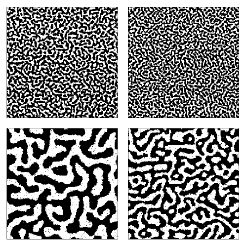
Figure 1: Evolution pictures for phase separation in a binary (AB) mixture with a critical composition. The component A ($\sigma=+1$) is marked in black, and the component B ($\sigma=-1$) is unmarked. The system was quenched at time $t=0$ from $T=\infty$ to $T=0.63T_{c}$. The top and bottom panels show snapshots at times $t=10^{4}$ and $10^{6}$ MCS, using either Model B dynamics (left), or Model S dynamics (right). The MC simulations were done on square lattices of size $512^{2}$ with periodic boundary conditions. The details of the simulations are described in the text.

time evolution for a critical composition (50 % A and 50 % B) after a quench to $T=0.63T_{c}$ for Model B (left) and Model S (right). Notice that the evolution morphology has a characteristic domain size, which we denote as $R(t)$. The growth process is substantially slower for S-dynamics, as expected. We will demonstrate shortly that the growth law due to bulk diffusion is $R(t)\sim t^{1/3}$, which is referred to as the Lifshitz-Slyozov (LS) growth law. The corresponding law for segregation via surface diffusion is $R(t)\sim t^{1/4}$. However, we reiterate that bulk diffusion is not eliminated entirely in Model S because of the presence of impurity spin clusters in bulk domains. At high temperatures, there is a reasonable fraction of impurity spins and we expect the S-dynamics to cross over to $t^{1/3}$-growth at late times. The crossover time increases rapidly at lower temperatures where there are very few impurity spins in the bulk as $P_{\rm{imp}}\simeq\left[1+\exp(8\beta J)\right]^{-1}$ in $d=2$.

We will study the evolution depicted in Fig. 1 using quantities like the correlation function and autocorrelation function.

3.1 Growth Laws

The first relevant property is the growth law governing the segregation process. We computed the typical domain size $R(t)$ as the first zero-crossing of the two-point correlation function:

$$C(\vec{r},t) = {1\over N}\sum_{i=1}^{N}\left[\langle\sigma_{i}(t)\sigma_{i+\vec{r}}(t)\rangle-\langle\sigma_{i}(t)\rangle\langle\sigma_{i+\vec{r}}(t)\rangle\right]$$ (9)

$$\equiv g\left({r\over R}\right).$$ (10)

Here, $\vec{r}$ denotes the displacement vector, and we consider systems which are translationally invariant and isotropic. The angular brackets in Eq. (9) denote an averaging over independent initial conditions and noise realizations. Equation (10) is the dynamical-scaling property of the correlation function [25], and reflects the fact that the morphology is self-similar in time, upto a scale factor (see Fig. 1). One can use other definitions of the length scale also, but these are all equivalent in the scaling regime.

At this stage, it is useful to clarify the domain growth laws which arise due to bulk and surface diffusion. A convenient starting point is the CHC equation (3) with an order-parameter-dependent mobility $D(\psi)$. We consider a general situation where the diffusion coefficient at the interface ($\psi=0$) is $D_{s}$, and that in the bulk [$\psi=\psi_{s}(T)$] is $D_{b}$ with $D_{b}\leq D_{s}$. This difference in surface and bulk mobilities may be the consequence of low-temperature dynamics or due to physical processes like glass formation or gelation. Then, the simplest functional form which models the mobility is

$$D(\psi)=D_{s}\left(1-\alpha\frac{\psi^{2}}{\psi_{s}^{2}}\right),\quad\alpha=1-\frac{D_{b}}{D_{s}},$$ (11)

which is equivalent to Eq. (5) with $D_{0}=D_{s}$ and $\psi_{0}^{2}=\psi_{s}^{2}/\alpha$. We focus on the deterministic case of Eq. (3):

$$\frac{\partial}{\partial t}\psi(\vec{r},t)=D_{s}\vec{\nabla}\cdot\left\{\left(1-\alpha\frac{\psi^{2}}{{\psi_{s}}^{2}}\right)\vec{\nabla}\left[-(T_{c}-T)\psi+\frac{T_{c}}{3}\psi^{3}-J\nabla^{2}\psi\right]\right\},$$ (12)

where we have used the $\psi^{4}$-form of the free energy from Eq. (4). The saturation value of the order parameter in Eq. (12) is $\psi_{s}(T)=\sqrt{3\left(1-T/T_{c}\right)}$. Using the natural scales for the order parameter, length and time, we can rewrite Eq. (12) in the dimensionless form:

$$\frac{\partial}{\partial t}\psi(\vec{r},t)=\vec{\nabla}\cdot\left[\left(1-\alpha\psi^{2}\right)\vec{\nabla}\left(-\psi+\psi^{3}-\nabla^{2}\psi\right)\right],$$

$$\alpha\in[0,1]~{}~{}\mbox{for}~{}~{}D_{b}\leq D_{s}.$$ (13)

The RHS of Eq. (3.1) can be decomposed as [20]

$$\frac{\partial}{\partial t}\psi(\vec{r},t) = (1-\alpha)\nabla^{2}(-\psi+\psi^{3}-\nabla^{2}\psi)+$$ (14)

$$\alpha\vec{\nabla}\cdot\left[\left(1-\psi^{2}\right)\vec{\nabla}\left(-\psi+\psi^{3}-\nabla^{2}\psi\right)\right],$$

where the first term on the RHS corresponds to bulk diffusion. This term disappears for $\alpha=1$ or $D_{b}=0$. The second term on the RHS corresponds to surface diffusion and is only operational at interfaces where $\psi\simeq 0$. Following Ohta [26], we can obtain an equation which describes the interfacial dynamics. The location of the interfaces $\vec{r}_{i}(t)$ is defined by the zeros of the order-parameter field:

$$\psi\left[\vec{r}_{i}(t),t\right]=0.$$ (15)

Focus on a particular interface, and designate the normal coordinate as $n$ (with dimensionality 1) and the interfacial coordinates as $\vec{a}$ [with dimensionality $(d-1)$]. Then, the normal velocity $v_{n}(\vec{a},t)$ obeys the integro-differential equation [26, 20]:

$$4\int d\vec{a^{\prime}}G[\vec{r}_{i}(\vec{a}),\vec{r}_{i}(\vec{a^{\prime}})]v_{n}(\vec{a^{\prime}},t) \simeq (1-\alpha)\sigma K(\vec{a},t)+$$ (16)

$$4\alpha\int d\vec{a^{\prime}}G[\vec{r}_{i}(\vec{a}),\vec{r}_{i}(\vec{a^{\prime}})]\nabla^{2}K(\vec{a^{\prime}},t),$$

where $K(\vec{a},t)$ is the local curvature at point $\vec{a}$ on the interface, and $\sigma$ is the surface tension. The Green’s function $G(\vec{x},\vec{x^{\prime}})$ obeys

$$-\nabla^{2}G(\vec{x},\vec{x^{\prime}})=\delta(\vec{x}-\vec{x^{\prime}}).$$ (17)

A dimensional analysis of Eq. (16) in the scaling regime yields the growth laws due to surface and bulk diffusion. We identify the scales of various quantities in Eq. (16) as

$$[d\vec{a}]\sim R^{d-1},\quad[G]\sim R^{2-d},$$

$$[v_{n}]\sim\frac{dR}{dt},\quad[K]\sim R^{-1}.$$ (18)

This yields the crossover behavior of the length scale as

$$R(t) \sim (\alpha t)^{1/4},\quad t\ll t_{c},$$ (19)

$$\sim [(1-\alpha)\sigma t]^{1/3},\quad t\gg t_{c},$$

where the crossover time is

$$t_{c}\sim\frac{\alpha^{3}}{(1-\alpha)^{4}\sigma^{4}}.$$ (20)

The above scenario applies for both Models B and S, as $D_{b}<D_{s}$ in either case. At moderate temperatures, this crossover occurs rapidly for Model B in our simulations. However, in Model S, there is a drastic suppression of bulk diffusion with $D_{b}\ll D_{s}$ and $\alpha\simeq 1$. Therefore, the crossover to $t^{1/3}$-growth is strongly delayed and not observed over simulation time-scales. This is seen in Fig. 2, which plots $R$ vs. $t$

Figure 2: Typical domain size ($R$) as a function of time ($t$) after a quench at $t=0$ from $T=\infty$ to $T=0.63T_{c}$ (left) and $0.88T_{c}$ (right). The circles and squares indicate data obtained with Model B and Model S dynamics, respectively. Lines with slope $1/4$ and $1/3$ are also provided on the plots as guides to the eye.

at temperatures $T=0.63T_{c}$ and $0.88T_{c}$ for Models B and S. The data for Model S is consistent with the growth law $R\sim t^{1/4}$. The early-time data for Model B is also consistent with this growth law, as surface diffusion is dominant at early times. At late times, one sees crossover behavior between the $t^{1/4}$-regime and the asymptotic $t^{1/3}$-regime. Note that the crossover for Model B is delayed at the higher temperature $T=0.88T_{c}$ because the decrease in $\alpha$ is more than compensated by the reduction in $\sigma$ due to softening of the interfaces as $T\rightarrow T_{c}^{-}$ [see Eq. (20)]. More generally, we stress that it has been notoriously difficult to observe the asymptotic $t^{1/3}$-growth in MC simulations of the Kawasaki model [11, 12]. Similar results have been obtained from Langevin studies of coarse-grained models [18, 19, 20].

Before proceeding, we remark that we have also studied models where bulk diffusion is more strictly suppressed by imposing additional kinetic constraints which eliminate 2-spin diffusion, 3-spin diffusion, etc. The corresponding results for the growth law are numerically indistinguishable from the Model S results in Fig. 2 over the time-scales of our simulation. This underlines the utility of the proposed Model S in the context of phase separation via surface diffusion.

It is also relevant to discuss off-critical quenches, where one of the components is present in a larger fraction. In Fig. 3, we show evolution pictures for Models B and S for the case with 25% A and 75% B.

Figure 3: Analogous to Fig. 1, but for an off-critical quench with 25% A and 75% B. The temperature is $T=0.63T_{c}$.

If the evolution morphology is not bicontinuous, e.g., there are droplets of the minority phase in a matrix of the majority phase, the surface-diffusion mechanism is unable to drive growth. Nevertheless, at high temperatures, growth may still proceed by the Brownian motion of droplets [27]. The corresponding growth law depends explicitly on the dimensionality:

$$R(t)\sim(Tt)^{1/(d+2)}.$$ (21)

Thus, domain growth through droplet motion obeys the law $R(t)\sim(Tt)^{1/4}$ in $d=2$, which is analogous to the surface-diffusion growth law. The growth kinetics of Models B and S for off-critical mixtures at $T=0.63T_{c}$ is shown in Fig. 4. We see that the S-dynamics shows the expected $t^{1/4}$-growth over extended time-regimes. As before, the B-dynamics shows a crossover behavior between the $t^{1/4}$-regime and the asymptotic $t^{1/3}$-regime. At low temperatures, the Brownian mechanism is ineffective and the evolution of Model S freezes into a meso-structure.

Figure 4: Analogous to Fig. 2, but for an off-critical quench with 25% A and 75% B. We show results for $T=0.63T_{c}$.

3.2 Correlation Functions

Next, let us study the morphological features of the evolution in Figs. 1 and 3. These are usually characterized by (a) the correlation function defined in Eq. (9), or (b) its Fourier transform, the structure factor. We have confirmed that these quantities exhibit dynamical scaling for both Models B and S. For the sake of brevity, we do not show these results here.

An important theme in this context is a comparison of the morphologies arising from both dynamics. Earlier studies with coarse-grained models [18, 19, 20] have found that the correlation functions and structure factors are numerically indistinguishable for growth driven by bulk diffusion or surface diffusion. At the visual level, this also seems to be suggested by the snapshots in Figs. 1 and 3. In Fig. 5, we compare the scaling

Figure 5: Superposition of scaling functions for Models B (solid line) and S (dashed line) for the evolution depicted in Fig. 1. For Model S, the data set corresponds to $t=10^{6}$ MCS; for Model B, the data set corresponds to $t=3.4\times 10^{5}$ MCS. Both domain sizes coincide at these times. (a) Plot of $C(r,t)$ vs. $r/R$. (b) Plot of $C(r,t)\cdot(r/R)$ vs. $r/R$, so as to magnify the tail behavior.

functions for Models B and S for a critical quench with $T=0.63T_{c}$. To eliminate finite-size effects, we consider cases with the same typical domain size: $t=10^{6}$ MCS in Model S and $t=3.4\times 10^{5}$ MCS in Model B. In Fig. 5(a), we plot $C(r,t)$ vs. $r/R$. The scaling functions superpose on the scale of the plot, in accordance with earlier studies of phenomenological models. In Fig. 5(b), we plot $C(r,t)\cdot(r/R)$ vs. $r/R$ so that the large-distance behavior is magnified. Some subtle differences between the two functions are seen at large distances $r/R>2$. We make some observations in this regard:
(a) The statistical error in the difference between the curves at the second peak is about four times smaller than the difference, so it cannot be attributed to statistical fluctuations.
(b) We have also replotted the correlation functions for Models B and S from different times on the scale $C(r,t)\cdot(r/R)$ vs. $r/R$. In that case, the secondary peaks show a much better collapse, suggesting that the discrepancy in Fig. 5(b) is not the result of corrections to scaling.

Though it is difficult to attribute physical significance to these differences, it is conceptually important to stress the observable differences between the morphologies for Models B and S. Similar scaling plots for the off-critical quench shown in Fig. 3 are shown in Fig. 6.

Figure 6: Analogous to Fig. 5, but for an off-critical quench with 25% A and 75% B at $T=0.63T_{c}$. In this case, the times for the different data sets are $t=9.8\times 10^{5}$ MCS (Model S) and $t=2.7\times 10^{5}$ MCS (Model B).

It is known that the scaling functions for phase-separating systems depend on the degree of off-criticality [28]. Notice that the oscillations in the plot of $C(r,t)$ vs. $r/R$ diminish with increase in the off-criticality. Further, the discrepancy between the scaling functions for Models B and S is larger for the off-critical case.

3.3 Island Distribution and Excess Energy

Our subsequent results will focus on the case of a critical quench. An alternative method of describing the domain morphology is the island-size distribution. We define an island as a set of aligned spins, all of whose neighbors are either part of the island, or have an antiparallel spin. Tafa et al. [29] have shown that the domain-size distribution in a phase-separating system $\widetilde{P}(l,t)$ exhibits scaling, and has an exponential decay:

$$\widetilde{P}(l,t)=R^{-1}f\left(\frac{l}{R}\right),\quad f(x)\sim e^{-ax}~{}~{}\mbox{for}~{}~{}x\rightarrow\infty,$$ (22)

where $l$ is the domain size and $a$ is a constant. The corresponding scaling form for the island-size distribution $P(s,t)$ in $d=2$ is obtained as

$$P(s,t) = \int_{0}^{\infty}dl\delta(s-bl^{2})\widetilde{P}(l,t)$$ (23)

$$= \langle s\rangle^{-1}~{}g\left(\frac{s}{\langle s\rangle}\right),\quad g(x)=\frac{1}{2\sqrt{x}}f(\sqrt{x}),$$

where $b$ is a geometric factor, and $\langle s\rangle$ is the average island size.

In Fig. 7, we plot

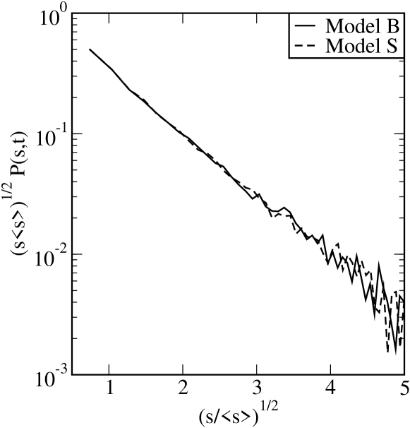
Figure 7: Scaled probability distributions for island-sizes in Models B (solid line) and S (dashed line) at $T=0.88T_{c}$. The data is shown on a linear-log plot as $\sqrt{s\langle s\rangle}P(s,t)$ vs. $\sqrt{s/\langle s\rangle}$, suggested by Eqs. (22)-(23). For Model S, the data set corresponds to $t=10^{6}$ MCS; for Model B, the data set corresponds to $t=3.4\times 10^{5}$ MCS. Both domain sizes coincide at these times.

$\sqrt{s\langle s\rangle}P(s,t)$ vs. $\sqrt{s/\langle s\rangle}$ for both Models B and S. We make two observations in this context. First, the data for the two models is numerically indistinguishable on the scale of this plot. The subtle differences in the correlation-function data are not seen in the island-size distribution function. Second, the plot in Fig. 7 exhibits an exponential decay, as expected from Eqs. (22)-(23).

A macroscopic quantity which depends on the density of small islands is the total energy $E(t)$. The interfacial energy for a domain is $\sigma R^{d-1}$, and the number of domains in the system $\sim N/R^{d}$. Thus, the overall interfacial energy depends on the length scale as $E(t)-E(\infty)\sim N\sigma/R$. In Fig. 8, we plot

Figure 8: Plot of the energy per site $E(t)/N$ vs. $R^{-1}$ for Model B at temperatures $T=0.63T_{c}$ (squares) and $T=0.88T_{c}$ (circles), and Model S at the same two temperatures (diamonds and crosses).

$E(t)/N$ vs. $R^{-1}$ for both Models B and S at $T=0.63T_{c}$ and $0.88T_{c}$. We observe a power-law convergence of the excess energy with the slope being proportional to the surface tension $\sigma(T)$. Again, the data sets at the same temperature cannot be distinguished on the scale of the plot.

3.4 Aging of the Autocorrelation Function

The data presented so far has focused on the morphological features of the phase-separating system. Let us next study the temporal correlation of the pattern dynamics in Fig. 1. This is measured by the autocorrelation function:

$$A(t_{w},\tau) = {1\over N}\sum_{i=1}^{N}\left[\langle\sigma_{i}(t_{w})\sigma_{i}(t_{w}+\tau)\rangle-\langle\sigma_{i}(t_{w})\rangle\langle\sigma_{i}(t_{w}+\tau)\rangle\right],$$ (24)

where the times $t_{w}$ and $(t_{w}+\tau)$ are measured after the quench at $t=0$. Here, $t_{w}$ is the reference time for measurement of the autocorrelation function, and is referred to as the waiting time. The most general correlation function corresponds to unequal space and time, and combines the definitions in Eqs. (9) and (24). Equilibrium systems are stationary and the corresponding $A(t_{w},\tau)$ only depends upon the time-difference $\tau$. On the other hand, for nonequilibrium systems, $A(t_{w},\tau)$ depends on both $t_{w}$ and $\tau$.

There have been some earlier studies of $A(t_{w},\tau)$ for domain growth in kinetic Ising models. There are two mechanisms which drive the decorrelation process:
(a) First, there are fluctuations in bulk domains, which give a stationary contribution. Huse and Fisher [30] studied decorrelation arising from the appearance of a droplet of (say) down-spins in an up-domain. The probability that a droplet of size $R$ appears via fluctuations is $P_{d}\propto\exp(-\beta\sigma R^{d-1})$. The lifetime of this droplet is $\tau\sim R^{1/\phi}$, where $\phi$ is the growth exponent. Thus, the corresponding autocorrelation function shows a stretched-exponential behavior:

$$A_{\rm{eq}}(\tau)\simeq\exp(-\beta\sigma\tau^{\theta}),$$

$$\theta=(d-1)\phi~{}\mbox{for}~{}d<d_{c}~{}\mbox{and}~{}1~{}\mbox{for}~{}d>d_{c}.$$ (25)

Here, the critical dimensionality is defined by $(d_{c}-1)\phi=1$.
(b) Second, there is decorrelation due to domain-wall motion. This can be either stochastic (due to thermal fluctuations) or systematic (due to the curvature-reduction mechanism). Consider the $T=0$ case, where there are no fluctuations in the bulk or the surface. The characteristic domain-wall velocity decreases with time, so this mechanism gives a non-stationary or aging ($t_{w}$-dependent) contribution [31]. Fisher and Huse [32] used scaling ideas to argue that the aging contribution to $A(t_{w},\tau)$ has a power-law dependence on the length scale:

$$A_{\rm{age}}(t_{w},\tau)=\left[{R(t_{w})\over R(t_{w}+\tau)}\right]^{\lambda},\quad R(t_{w}+\tau)\gg R(t_{w}).$$ (26)

There have been various studies of the aging exponent $\lambda$ in cases with both spin-flip and spin-exchange kinetics [1]. For power-law domain growth, Eq. (26) obeys the scaling form $A_{\rm{age}}(t_{w},\tau)=h(\tau/t_{w})$, which has been observed in some studies of spin glasses [31].

In Fig. 9, we plot $A(t_{w},\tau)$ vs. $\tau$ for Models B and S for a critical quench to

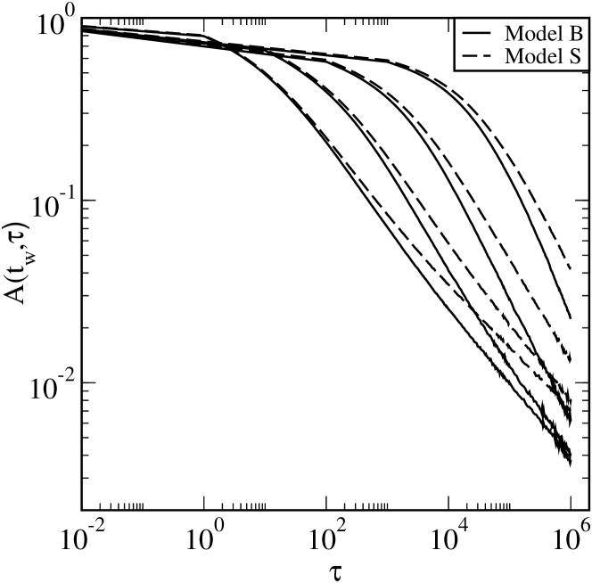
Figure 9: Time-dependence of the autocorrelation function for Models B (solid line) and S (dashed line) at $T=0.63T_{c}$. The waiting times are $t_{w}=10^{2},10^{3},10^{4},10^{5}$ MCS (from left to right).

$T=0.63T_{c}$. The solid lines denote data for Model B with waiting times $t_{w}=10^{2},10^{3},10^{4},10^{5}$ (from left to right). The dashed lines denote the corresponding data for Model S. As expected, the autocorrelation function decays more rapidly for Model B. We make the following observations in this regard:
(a) The quantity $A(t_{w},\tau)$ exhibits aging, with an explicit dependence on $t_{w}$ for both Models B and S. In general, the decay is slower for larger $t_{w}$, i.e., when the domain size of the reference state is larger. Further, the decay is faster for higher temperatures, where larger fluctuations are present in the system.
(b) The data in Fig. 9 is plotted on a log-log scale, and exhibits a continuous curvature for both Models B and S. This is not consistent with the simple power-law decay in Eq. (26). As a matter of fact, the autocorrelation data does not even exhibit $\tau/t_{w}$-scaling, as we have confirmed. In the case of Model B, this is because the decorrelation process is driven by both bulk fluctuations (with a stationary contribution) and domain-wall motion (with a non-stationary contribution). In the case of Model S, bulk fluctuations have been effectively eliminated and one may naively expect to recover power-law decay. However, this is not the case because interfacial fluctuations also contribute to decorrelation. We believe that the scaling behavior in Eq. (26) is only realized in kinetic Ising models or their coarse-grained analogs at $T=0$. In this limit, coarsening occurs only through the systematic motion of interfaces and the system always reduces its energy. However, the $T=0$ limit is not interesting in the context of kinetic Ising models because the evolving system invariably gets trapped in local free-energy minima.
(c) In recent work, Puri and Kumar [33] have studied the decorrelation process in a spin-1 model using a stochastic model based on the continuous-time random walk formalism. We are currently trying to adapt their modeling to understand the behavior in Fig. 9.

4 Summary and Discussion

Let us conclude this paper with a summary and discussion of the results presented here. We have studied phase separation in a kinetic Ising model for phase separation mediated by surface diffusion. This model (referred to as Model S) is obtained by imposing a kinetic constraint on the usual Kawasaki kinetic Ising model (referred to as Model B). In general, the surface diffusion mechanism can drive segregation only when the morphology consists of percolated clusters, i.e., for near-critical quenches. We have undertaken Monte Carlo (MC) simulations of Models B and S using multi-spin coding techniques. These provide accelerated algorithms which enable the simulation of large systems for extended times. Our results show that the major difference between the morphologies of Models B and S lies in the growth dynamics. In this regard, it is relevant to emphasize the following:
(a) The early-time dynamics ($t\ll t_{c}^{B}$) of Model B is also dominated by surface diffusion with the growth law $R(t)\sim t^{1/4}$. For late times ($t\gg t_{c}^{B}$), there is a crossover to the $t^{1/3}$-growth regime. In the limit of $T\rightarrow 0$, the crossover time diverges ($t_{c}^{B}\rightarrow\infty$). However, the low-temperature dynamics of Model B usually freezes into metastable states. Therefore, it is hard to see an extended regime of $t^{1/4}$-growth in Model B.
(b) Our kinetic constraint eliminates single-particle bulk diffusion, and we see extended regimes of growth driven by surface diffusion. However, $n$-particle diffusion (with $n\geq 2$) is still possible and is governed by the probability for existence of impurities in bulk domains. Thus, at sufficiently large times ($t\gg t_{c}^{S}$), we again expect a crossover to $t^{1/3}$-growth. However, this crossover is extremely delayed, even at moderate temperatures.
(c) We have also studied kinetic models with constraints which eliminate the diffusion of $n$-spin clusters. The domain growth data obtained from these models is numerically indistinguishable from that for Model S.
(d) For highly off-critical quenches, the morphology consists of droplets of the minority phase in a matrix of the majority phase. In this case, the surface diffusion mechanism cannot drive phase separation. However, Brownian motion and coalescence of droplets also gives rise to $t^{1/4}$-growth in $d=2$.

Apart from growth laws, we have also studied quantitative properties of the evolution morphology like correlation functions and island-size distribution functions. There are subtle differences in the scaled correlation functions for Models B and S, but it is difficult to attribute physical significance to these. Further, these differences are not reflected in the island-size distribution function.

Finally, we have studied the aging of the autocorrelation function $A(t_{w},\tau)$ in Models B and S. In both cases, we find that the decorrelation process is driven by both fluctuations and domain-wall motion. Thus, $A(t_{w},\tau)$ does not exhibit a simple power-law decay or scaling behavior. We are presently adapting the continuous-time random walk approach developed by Puri and Kumar [33] to study the aging of the autocorrelation functions in Models B and S.

References

- [1] A.J. Bray, Adv. Phys. 43, 357 (1994).
- [2] K. Binder and P. Fratzl, in Phase Transformations in Materials, edited by G. Kostorz (Wiley-VCH, Weinheim, 2001), p. 409.
- [3] A. Onuki, Phase Transition Dynamics (Cambridge University Press, Cambridge, 2002).
- [4] S. Dattagupta and S. Puri, Dissipative Phenomena in Condensed Matter: Some Applications, to be published by Springer-Verlag.
- [5] S. Puri, Phys. Rev. E 55, 1752 (1997); S. Puri and R. Sharma, Phys. Rev. E 57, 1873 (1998).
- [6] E.D. Siggia, Phys. Rev. A 20, 595 (1979); H. Furukawa, Phys. Rev. A 31, 1103 (1985).
- [7] S. Puri, D. Chowdhury and N. Parekh, J. Phys. A 24, L1087 (1991); S. Puri and N. Parekh, J. Phys. A 25, 4127 (1992).
- [8] A. Onuki and S. Puri, Phys. Rev. E 59, R1331 (1999).
- [9] K. Kawasaki, in Phase Transitions and Critical Phenomena Vol. 2, ed. by C. Domb and M.S. Green (Academic Press, London, 1972), p. 443.
- [10] K. Binder and D.W. Heermann, Monte Carlo Simulation in Statistical Physics: An Introduction, Fourth Edition (Springer-Verlag, Berlin, 2002).
- [11] J. Amar, F. Sullivan and R.D. Mountain, Phys. Rev. B 37, 196 (1988); and references therein.
- [12] J.F. Marko and G.T. Barkema, Phys. Rev. E 52, 2522 (1995); and references therein.
- [13] P.C. Hohenberg and B.I. Halperin, Rev. Mod. Phys. 49, 435 (1977).
- [14] K. Binder, Z. Phys. 267, 313 (1974).
- [15] J.S. Langer, M. Bar-on and H.D. Miller, Phys. Rev. A 11, 1417 (1975).
- [16] K. Kitahara and M. Imada, Prog. Theor. Phys. Suppl. 64, 65 (1978); K. Kitahara, Y. Oono and D. Jasnow, Mod. Phys. Lett. B 2, 765 (1988).
- [17] S. Puri, K. Binder and S. Dattagupta, Phys. Rev. B 46, 98 (1992); S. Puri, N. Parekh and S. Dattagupta, J. Stat. Phys. 77, 839 (1994).
- [18] S. Puri, A.J. Bray and J.L. Lebowitz, Phys. Rev. E 56, 758 (1997).
- [19] C. Yeung, Some Problems on Spatial Patterns in Nonequilibrium Systems, Ph.D. Thesis, Illinois (1989).
- [20] A.M. Lacasta, A. Hernandez-Machado, J.M. Sancho and R. Toral, Phys. Rev. B 45, 5276 (1992); A.M. Lacasta, J.M. Sancho, A. Hernandez-Machado and R. Toral, Phys. Rev. B 48, 6854 (1993).
- [21] D. Sappelt and J. Jackle, Europhys. Lett. 37, 13 (1997); Polymer 39, 5253 (1998).
- [22] F. Sciortino, R. Bansil, H.E. Stanley and P. Alstrom, Phys. Rev. E 47, 4615 (1993).
- [23] J. Sharma and S. Puri, Phys. Rev. E 64, 021513 (2001).
- [24] M.E.J. Newman and G.T. Barkema, Monte Carlo Methods in Statistical Physics (Oxford University Press, Oxford, 1999).
- [25] K. Binder and D. Stauffer, Phys. Rev. Lett. 33, 1006 (1974).
- [26] T. Ohta, J. Phys. C 21, L361 (1988); K. Kawasaki and T. Ohta, Prog. Theor. Phys. 68, 129 (1982).
- [27] H. Furukawa, Phys. Rev. A 29, 2160 (1984).
- [28] S. Puri, Phys. Lett. A 134, 205 (1988).
- [29] K. Tafa, S. Puri and D. Kumar, Phys. Rev. E 63, 046115 (2001); Phys. Rev. E 64, 056139 (2001).
- [30] D.A. Huse and D.S. Fisher, Phys. Rev. B 35, 6841 (1987).
- [31] J.-P. Bouchaud, L.F. Cugliandolo, J. Kurchan and M. Mezard, in Spin Glasses and Random Fields, ed. by A.P. Young (World Scientific, Singapore 1997), p. 161.
- [32] D.S. Fisher and D.A. Huse, Phys. Rev. Lett. 56, 1601 (1986); Phys. Rev. B 38, 373, 386 (1988).
- [33] S. Puri and D. Kumar, Phys. Rev. Lett. 93, 025701 (2004); Phys. Rev. E 70, 051501 (2004).