Steady States of a Microwave Irradiated Quantum Hall Gas

Abstract

We consider effects of a long-wavelength disorder potential on the Zero Conductance State (ZCS) of the microwave-irradiated 2D electron gas. Assuming a uniform Hall conductivity, we construct a Lyapunov functional and derive stability conditions on the domain structure of the photo-generated fields. We solve the resulting equations for a general one-dimensional and certain two-dimensional disorder potentials, and find non-zero conductances, photo-voltages, and circulating dissipative currents. In contrast, weak white noise disorder does not destroy the ZCS, but induces mesoscopic current fluctuations.

The observation of giant magnetoresistance oscillations in a microwave-irradiated two-dimensional electron gas (2DEG) ZRS-exp , has spurred intensive theoretical activity. Two distinct microscopic mechanisms for conductivity corrections have been proposed: (i) The displacement photocurrent (DP)ZRS-DP , which is caused by photo-excitation of electrons into displaced guiding centers and (ii) the distribution function (DF) mechanism, which involves redistribution of intra-Landau level population for large inelastic lifetimesZRS-DF .

Andreev, Aleiner and MillisZRS-macro have noted that irrespective of microscopic details, once the radiation is strong enough to render the local conductivity negative, the system as a whole will break into domains of photogenerated fields and spontaneous Hall currents. In their proposed domain phase, motion of domain walls can accommodate the external voltage, resulting in a Zero Conductance State (ZCS) in the Corbino geometry, or a Zero Resistance State for the Hall bar geometry, in apparent agreement with experimental reportsZRS-exp . However, one may ask, what should be the effects of long-wavelength (relative to the cyclotron radius) disorder, which is either naturally present or deliberately introduced? What is the nature of the coupling between a disorder potential and the photogenerated fields ZRS-disorder , and could the disorder pin domain walls? Such pinning would affect the macroscopic transport and could destroy the ZCS.

In this Letter we incorporate a long-wavelength disorder potential $\phi_{d}({\bf x})$ into the non-linear magneto-transport equations. We explore its effects on the domain structure and macroscopic transport coefficients. For the case of a constant Hall conductivity, we construct a Lyapunov functional Lyapunov which greatly simplifies the determination of the stable steady states and their conductance. We use it to derive general stability conditions on domain walls in the strong radiation regime. We also show that weak ’white-noise’ disorder is an irrelevant perturbation, which does not destroy the ZCS. It does introduce, however, mesoscopic non linear current fluctuations. We find solutions for the following disorder potentials: (i) The general one-dimensional potential, where domain walls are pinned to the potential extrema, which results in a non zero conductance and photo-voltage. (ii) The simple “egg-carton” potential solved variationally, and (iii) a generic non-separable potential depicted in Fig. 1, which is solved numerically. (ii) and (iii) exhibit two-dimensional domain wall pinning and frustration effects, which result in circulating dissipative currents.

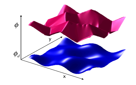
Figure 1: Domain phase in the presence of disorder: the photogenerated potential $\phi(x,y)$ corresponding to a generic long-wavelength disorder potential $\phi_{d}$. The steady state is determined by numerically minimizing the Lyapunov functional (see text). The domain walls (potential edges) are pinned by $\phi_{d}$, yielding a finite conductance.

Non-Linear Magneto-Transport. In the presence of an external microwave field, we use a local relation between the dc current ${\bf j}({\bf r})$ and the local electrostatic field ${\bf E}({\bf r})$:

$${\bf j}={\bf j}^{d}({\bf E},{\bf r})+\sigma^{H}\hat{{\bf z}}\times{\bf E}\ .$$ (1)

Here we assume at the outset that the Hall conductivity $\sigma^{H}$ is a constant, independent of ${\bf r}$ and ${\bf E}$, which leads to considerable simplifications. The dissipative conductivity, $\sigma^{d}_{\alpha\beta}({\bf E})\equiv\partial j^{d}_{\alpha}/\partial E_{\beta}$, satisfies

$$\sigma^{d}_{\alpha\beta}({\bf E},{\bf r})=\sigma^{d}_{\beta\alpha}({\bf E},{\bf r}).$$ (2)

The vector function ${\bf j}^{d}$, in general, will depend explicitly on the position ${\bf r}$, due, e.g., to inhomogeneities in the 2DEG, and its direction may not be perfectly aligned with ${\bf E}$. Eq. (1) is supplemented by the continuity equation, $\nabla\cdot{\bf j}=-\dot{\rho}$, where $\rho$ is the charge density. We emphasize that equation (1) contains all microscopic interactions at lengthscales shorter than the cyclotron radius $l_{c}$, which serves as an ultra-violet cut-off, of order 1$\mu$m.

Writing ${\bf E}\equiv-\nabla\phi$, we may relate changes in the electrostatic potential $\phi$ to changes in $\rho$ through the inverse capacitance matrix $W$:

$$\delta\phi({\bf r})=\int d^{2}r^{\prime}W({\bf r},{\bf r}^{\prime})\delta\rho({\bf r}^{\prime}).$$ (3)

If a time-independent steady state is reached, then we have simply $\nabla\cdot{\bf j}=0$, and the precise form of $W$ is unimportant.

In a Corbino geometry, one specifies the potential on the inner and outer boundaries of the sample, and one looks for a solution for $\phi({\bf r})$ consistent with these boundary conditions. Since we asssume $\sigma^{H}$ to be a constant, the Hall current cannot contribute to $\nabla\cdot{\bf j}$ in the interior of the sample, so it does not appear in Kirchoff’s equations. Consequently, the solution for $\phi({\bf r})$ is independent of $\sigma^{H}$ and we may, for simplicity set $\sigma^{H}=0$. To recover the Hall current, one inserts the solution ${\bf E}$ into the second term in (1).

Condition (2) on ${\bf j}^{d}$ allows us to define a scalar Lyapunov functional as

$$G[\phi]=\int d^{2}rg({\bf E}),~{}~{}~{}g=\int_{0}^{{\bf E}({\bf r})}d{\bf E}^{\prime}\cdot{\bf j}^{d}({\bf E}^{\prime}).$$ (4)

A variation of (4) is given by

$$\delta G=\int d^{2}r\nabla\cdot{\bf j}^{d}~{}\delta\phi-\int_{bound}ds\hat{{\bf n}}\cdot{\bf j}^{d}\delta\phi.$$ (5)

The second integral vanishes on equipotential boundaries, or in the absence of external currents. The extrema of $G$ are found to be steady states, with $\nabla\cdot{\bf j}=0$. Using the positivity of the inverse capacitance matrix $W$, one may show that $G[\phi(t)]$ is indeed a Lyapunov functional, i.e. a non-increasing function of time, so that its minima are stable steady states. In general, $G$ may have multiple minima. Any initial choice of $\phi({\bf r})$ will relax to some local minimum of $G$, but not necessarily the “ground state” with lowest $G$. Nevertheless, we expect that in the presence of noise, the system might tend to escape from high-lying minima and wind up in a state with $G$ close to the absolute minimum.

Using the boundary term in (5), the current across a Corbino sample is equal to the first derivative of $G$ with respect to the potential difference $V$ between two edges, and the differential conductance is given by the stiffness, or the second derivative:

$${dI\over dV}={d^{2}G\over dV^{2}}.$$ (6)

The Domain Phase. We now consider a homogeneous system, in the regime of strong microwave radiation at frequencies slightly larger than the cyclotron harmonics $\omega>m\omega_{c},m=1,2,\ldots$ i.e. positive detuning. Both DP and DF mechanisms produce a regime of negative conductivity ${\bf j}({\bf E})\cdot{\bf E}<0$, which implies a minimum of $g(E)$ at a finite field $|{\bf E}|=E_{c}>0$, which was estimatedVA to be of order $\hbar\omega_{c}/(el_{c})$. In order to satisfy equipotential boundary conditions, and the constraints $\oint d{\bf l}\cdot{\bf E}=0$, field discontinuities and charge density singularities must form.

A second order expansion of $g$ about $E_{c}$ reads as

$$g_{0}({\bf E})=g_{0}(E_{c})+{1\over 2}(E-E_{c})^{2}\sigma_{c}+\lambda|\nabla\cdot{\bf E}|^{2}\ .$$ (7)

The clean system of Eq.(7), is governed by a ‘Mexican hat’ Lyapunov density, with a flat valley along $|{\bf E}|=E_{c}$, i.e. the steady state local conductivity is ‘marginally’ stable everywhere except inside the domain walls. The field-derivative coefficient $\lambda\approx\sigma_{c}l_{dw}^{2}$ implements the ultra-violet cut off, introducing a domain-wall thickness scale $l_{dw}$ assumed here to be of the order of $l_{c}$. Domain walls yield a positive contribution to $G$ of order $\sigma_{c}E_{c}^{2}l_{dw}$ per unit length. In the absence of disorder, the system will simply minimize total domain walls contribution, subject to aforementioned constraints.

A change in the average field $\langle{\bf E}\rangle$, required if there is a change in the applied voltage $V$, can be accommodated by a motion of domain walls, or a reorientation of the local ${\bf E}$. The relative corrections to zero conductance vanish as $l_{dw}$ over the sample length. This defines the clean ZCS phase described in Ref. ZRS-macro .

Long-Wavelength Disorder. In an inhomogeneous system, there will be a non-zero electrostatic field, ${\bf E}_{d}({\bf r})\equiv-\nabla\phi_{d}({\bf r})$, present in the thermal equilibrium state, with no microwave radiation or bias voltage. We may ask how this disorder field will alter the ZCS.

At weak disorder field, $|{\bf E}_{d}|<<E_{c}$, the Lyapunov density near $E\approx E_{c}$ is modified to

$$g({\bf E},{\bf E}_{d})=g_{0}({\bf E})-\sigma_{1}(E)~{}{\bf E}\cdot{\bf E}_{d}({\bf r})+{\cal O}(E_{d}^{2}),$$ (8)

which yields a current density

$${\bf j}^{d}({\bf r})=-\sigma_{1}{\bf E}_{d}+{g_{0}^{\prime}-\sigma_{1}^{\prime}{\bf E}\cdot{\bf E}_{d}\over E}{\bf E},$$ (9)

where $X^{\prime}\equiv\partial X/\partial E$, and the coefficient $\sigma_{1}$ depends on microscopic mechanisms.

We wish to elaborate on a physical issue regarding Eq.(9): In the non-irradiated (dark) linear response theory, the current is driven by the electrochemical gradient $\mbox{\boldmath$\mathbf{\epsilon}$ }={\bf E}-{\bf E}_{d}$. Similarly, one may expect the photocurrent of the DF mechanism to also depend on $\mathbf{\epsilon}$ . In contrast, the ’upstream’ photocurrent, pumped by the DP mechanism, involves transitions between single particle states which feel the local electric field ${\bf E}({\bf r})$. Thus, due to both contributions, even if the DP mechanism is relatively weak, ${\bf E}_{d}$ cannot be eliminated from Eq.(9) by a change of variables ${\bf E}\to\mbox{\boldmath$\mathbf{\epsilon}$ }$. By our microscopic estimateelsewhere , for the pure DP mechanism, $\sigma_{c},\sigma_{1}(E_{c})$ are close to the dark conductivity, and $\sigma_{1}^{\prime}<<\sigma_{c}/E_{c}$.

Local stability requires that $\sigma^{d}({\bf r})$, of Eq. (2), has non-negative eigenvalues. The lower (transverse) eigenvalue is given by

$$\sigma_{-}={g_{0}^{\prime}-\sigma_{1}^{\prime}{\bf E}\cdot{\bf E}_{d}\over E}+{\cal O}(E_{d})^{2}\geq 0\ ,$$ (10)

so marginal stability occurs at $E=E_{c}+\sigma_{1}^{\prime}{\bf E}_{d}\cdot{\bf E}/\sigma_{c}$.

In a steady state, the normal current density (in direction $\hat{{\bf n}}$) is continuous across a domain wall. If ${\bf E}_{1}$ and ${\bf E}_{2}$ are the fields on its two sides, we find by (10) and(8) that

$$\sigma_{-}(E_{1})~{}{\bf E}_{1}\cdot\hat{{\bf n}}=\sigma_{-}(E_{2})~{}{\bf E}_{2}\cdot\hat{{\bf n}}~{}+{\cal O}(E_{d}^{2}).$$ (11)

When ${\bf E}_{i}\cdot\hat{{\bf n}},i=1,2$ have opposite signs (as they do in the clean limit) (11) can only be satisfied for $\sigma_{-}(E_{1})=\sigma_{-}(E_{2})={\cal O}(E_{d})^{2}$. This restricts the fields at the domain wall to be at their respective marginally stable values. As a result, the current density (9) at the domain wall reduces to

$${\bf j}=-\sigma_{1}(E_{c}){\bf E}_{d}+{\cal O}(E_{d})^{2}$$ (12)

By Eq.(12), current conservation and Gauss’ theorem, and we obtain a global condition on any closed domain walls,

$$0=\oint{\bf n}\cdot{\bf j}=-2\pi\sigma Q^{2D}+{\cal O}(E_{d}^{2}),$$ (13)

where $Q^{2D}$ is the integral of the “2D disorder-charge density,” $\nabla\cdot{\bf E}_{d}/2\pi$, over the area enclosed by the loop.

Finally, we note that generically, the differential conductance of a sample in the Corbino geometry can be obtained by solving for the conductance of a linear system with local conductivity given by $\sigma^{d}({\bf E}({\bf r}))$, in series with resistive elements along the domain walls, which arise from movement of the domain walls in response to a variation in the applied bias $V$. (There could also be discontinuities in the current at discrete values of $V$, if the system jumps discontinuously from one local minimum of $G$ to another.) We shall see that for weak long-wavelength disorder, the scale of the macroscopic conductance is set by the domain-wall contribution.

White-Noise Disorder. In the ZCS, we now show that a weak ‘white-noise’ disorder potential, with a correlation length $\xi_{d}$ (of the order $l_{dw}\sim l_{c}$), and root-mean-square value ${\bar{\phi}_{d}}\ll E_{c}\xi_{d}$ is an irrelevant perturbation which does not introduce new domain walls or destroy the ZCS. This is shown by using an Imry-Ma comparisonImryMa of surface to bulk contributions to the Lyapunov functional. By (8), for a square domain of area $L_{d}^{2}$, the negative contribution of aligning ${\bf E}$ with the averaged disorder field ${\bf E}_{d}$, scales as $-\sigma_{1}{\bar{\phi}_{d}}E_{c}\sqrt{L_{d}\xi_{d}}$. However the linear cost of its domain walls grows as $+\sigma_{c}E_{c}L_{d}l_{dw}$. Therefore weak disorder cannot necessarily break the system up into smaller domains.

The disorder, however, will produce current fluctuations across pre-existing domain walls, needed to satisfy boundary conditions on the sample. By Eq. (12), the current density integrates across the domain wall to yield a random number of order

$$\delta I=\pm\sigma_{1}{\delta V{\bar{\phi}_{d}}\over E_{c}\xi_{d}^{5/2}}L_{d}^{1/2}$$ (14)

While the conductance will average out to zero at voltages $V\geq E_{c}\xi_{d}$ or if multiple domains are in series. The random currents and conductance fluctuations should be observable in small samples, or as harmonic noise generation for oscillatory bias voltage.

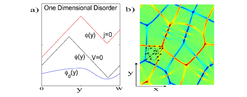
Figure 2: a) Photogenerated potential solutions $\phi$, for one dimensional disorder $\phi_{d}(y)$, with zero current and zero voltage boundary conditions. b) Map of $\nabla\cdot{\bf E}$ (red-positive, blue-negative) for solution $\phi(x,y)$ of Fig. 1, showing the domain walls. Circulating dissipative currents are illustrated in one domain.

One-Dimensional Disorder. In contrast to weak white-noise disorder, potentials with long-range correlations can be relevant perturbations. Consider the case of a general one-dimensional disorder (see Fig.2a), where $\phi_{d}(y)$ is independent of the $x$-coordinate. At wavelengths larger than $l_{dw}$ , the Lyapunov functional is minimized if the system breaks up into parallel domains, so that ${\bf E}$ is everywhere aligned with ${\bf E}_{d}$, and ${\bf j}^{d}=0$. These conditions determine ${\bf E}(y)$ via (9), and the boundary conditions for a rectangular Corbino geometry (periodic boundary conditions at $x=0$ and $x=L$). The voltage difference $V$ between the leads at $y=0$ and $y=W$ , satisfies

$$V(I)=\int_{0}^{W}dy(E(y)-E_{d}(y))\ .$$ (15)

At strong radiation intensity and zero current, (12) and transverse stability imposes that domain walls form precisely at maxima and minima of $\phi_{d}$, given by the $y_{i},i=1,\ldots,N$ To lowest order in $\phi_{d}$, there will be a non-zero photovoltage which only depends on these positions:

$$V(0)=E_{c}\left((-1)^{N}W-2\sum_{i=1}^{N}(-1)^{i}y_{i}\right)+{\cal O}(E_{d}),$$ (16)

where $i=1,3\ldots$ are maxima. The differential conductivity $\sigma_{yy}$ is given, to lowest order in $\phi_{d}$, by

$${1\over\sigma_{yy}}={2E_{c}\over\sigma_{1}W}\sum_{i}{1\over|\phi_{d}^{\prime\prime}(y_{i})|}\equiv{2E_{c}\over\sigma_{1}\tilde{E}_{d}}\ ,$$ (17)

If $P(E_{d})$ is the probability distribution for $E_{d}$ at a random point, it can be shown that $\tilde{E}_{d}^{-1}=P(0)$. If $E_{d}$ is taken from a Gaussian distribution, then $\tilde{E_{d}}=(2\pi)^{1/2}E_{d}^{\rm{rms}}$, where $E_{d}^{\rm{rms}}$ is the root-mean-square value of $E_{d}$. If $\phi_{d}$ is a single sine wave, then $\tilde{E_{d}}=2^{1/2}\pi E_{d}^{\rm{rms}}$. The transverse differential conductivity $\sigma_{xx}$ can also be calculated, using (10), and is given, to first order in $\phi_{d}$ by $\sigma_{xx}=\sigma_{1}\langle|{\bf E}_{d}|\rangle/E_{c}$. For a Gaussian distribution, one has $\sigma_{xx}=(2/\pi)\sigma_{yy}$, while for a single sine wave, $\sigma_{xx}=(4/\pi^{2})\sigma_{yy}$.

Two-Dimensional Potentials The simplest 2D choice for $\phi_{d}$ is the separable ‘egg-carton’ potential, given by

$$\phi_{d}={E^{0}_{d}\over\sqrt{2}}\left(\cos(x)+\cos(y)\right)\ .$$ (18)

We construct a zeroth order trial solution for zero bias current ${\bf j}^{d}_{0}=0$ by placing domain walls on the lines $x=n\pi$ and $y=m\pi$, for integer $n$ and $m$. This yields constant electric fields in each square domain, of the form:

$${\bf E}_{0}={E_{c}\over\sqrt{2}}(\pm\hat{x}\pm\hat{y})\ .$$ (19)

${\bf E}_{0}$ is a gradient of a continuous potential, and satisfies charge neutrality (13). Upon application of an external voltage in an arbitrary direction, domain walls will move, as in the one-dimensional case, and also tilt with ${\bf E}$ into a herringbone pattern. A variational calculation, assuming that within each domain ${\bf E}$ is constant, finds, to first order in $E_{d}$, that $\sigma_{xx}=0.83\sigma_{1}E^{0}_{d}/E_{c}$. Numerical calculations confirm that the variational solution is at least close to the exact answer.

We have calculated analytically the first order (in $E_{d}$) corrections to (19), for zero external voltage, by integrating Kirchoff’s lawselsewhere . Away from the domain walls, we find $E>E_{c}$, which corresponds to circulating dissipative currents, which match onto the tangential currents at domain walls, given by Eq. 12. In Fig. 1, a generic two dimensional example is displayed. $\phi_{d}$ contains 20 Fourier components chosen from Gaussian distributions with $<|\phi_{d}({\bf{k}}|^{2}>$ independent of ${\bf{k}}$. The potential $\phi$ is found by numerically minimizing $G$. Fig.  2b plots the 2D charge density where domain walls appear as line singularities. In both two dimensional examples, (18) and Fig.1, $G$ is frustrated from perfect alignment of ${\bf E}$ and ${\bf E}_{d}({\bf r})$ by the conditions $|{\bf E}|\geq E_{c}$ and $\nabla\times{\bf E}=0$. This frustration underlies the circulating dissipative currents which are illustrated in one of the domains in Fig. 2b.

In summary, we have introduced long wavelength disorder into the transport theory of the microwave irradiated quantum Hall gas, using the Lyapunov functional as an organizing principle for the stability of steady states. We showed that weak white noise disorder is irrelevant for the stability of the ZCS although it produces mesoscopic current fluctuations. For a strong and long range potentials, the ZCS state breaks up into domains, which will generally result in a finite conductance and a photovoltaic effect. A microscopic theory necessary for the steady states dependence on microwave power and detuning frequency is deferred to a forthcoming publicationelsewhere . We have not considered effects of conductivity anisotropy and variations in Hall coefficient. The latter will not affect the domain pattern or the longitudinal conductivity for one-dimensional disorder, but might have large effects and be experimentally relevant in other geometries.

Acknowledgment. We thank E. Meron, A. Stern, R. L. Willett and Y. Yacoby for helpful discussions. AA and AY are grateful for the hospitality of Harvard University, Aspen Center for Physics and Kavli Institute for Theoretical Physics. Work was supported in part by the Harvard Center for Imaging and Mesoscale Structures, NSF grant DMR02-33773, the US-Israel Binational Science Foundation, and the Minerva Foundation.

References

- (1) R. G. Mani et.al. Nature, 420, 646 (2002); M. A. Zudov et. al. Phys. Rev. Lett. 90, 046807 (2003); C. L. Yang et. al. Phys. Rev. Lett. 91, 096803 (2003); R. L. Willett, et. al. Bull. Am. Phys. Soc. 48, 459 (2003).
- (2) A. Durst, S. Sachdev, N. Read, and S. M. Girvin, Phys. Rev. Lett. 91, 086803 (2003); V. I. Rig, Fiz. Tverd. Tela 11 , 2577 (1969) [Sov. Phys. Solid State 11 , 2078 (1970)]; P.W. Anderson and W.F. Brinkman, cond-mat/0302129; J. Shi and X.C. Xie, Phys. Rev. Lett. 91, 086801 (2003).
- (3) I. A. Dmitriev, A. D. Mirlin and D. G. Polyakov, Phys. Rev. Lett. 91, 226802 (2003); I. A. Dmitriev, M.G.Vavilov, I. L. Aleiner, A .D. Mirlin and D. G. Polyakov, preprints cond-mat/0310668 and 0409590.
- (4) A.V. Andreev, I.L. Aleiner, and A.J. Millis, Phys. Rev. Lett. 91, 056803 (2003);
- (5) Effects of a short wavelength periodic potential have been recently addressed by by J. Dietel, L. Glazman, F. Hekking, F. von Oppen, cond-mat/0407298.
- (6) M.C. Cross and P.C. Hohenberg, Rev. Mod. Phys. 65, 851 (1993). The dynamical phase transition in J. Alicea, L. Balents, M.P.A. Fisher, A. Paramekanti, L. Radzihovsky, cond-mat/0408661, is governed by a Lyapunov functional.
- (7) M.G. Vavilov and I.L. Aleiner, Phys. Rev. B 69, 035303 (2004).
- (8) A. Auerbach, I. G. Finkler, B.I. Halperin, A. Yacoby, in preparation.
- (9) Y. Imry and S.-k. Ma, Phys. Rev. Lett. 35, 1399 (1975).