Towards a Theory of Scale-Free Graphs:
Definition, Properties, and Implications (Extended Version)
Technical Report CIT-CDS-04-006, Engineering & Applied Sciences Division
California Institute of Technology, Pasadena, CA, USA

Abstract

Although the “scale-free” literature is large and growing, it gives neither a precise definition of scale-free graphs nor rigorous proofs of many of their claimed properties. In fact, it is easily shown that the existing theory has many inherent contradictions and verifiably false claims. In this paper, we propose a new, mathematically precise, and structural definition of the extent to which a graph is scale-free, and prove a series of results that recover many of the claimed properties while suggesting the potential for a rich and interesting theory. With this definition, scale-free (or its opposite, scale-rich) is closely related to other structural graph properties such as various notions of self-similarity (or respectively, self-dissimilarity). Scale-free graphs are also shown to be the likely outcome of random construction processes, consistent with the heuristic definitions implicit in existing random graph approaches. Our approach clarifies much of the confusion surrounding the sensational qualitative claims in the scale-free literature, and offers rigorous and quantitative alternatives.

1 Introduction

One of the most popular topics recently within the interdisciplinary study of complex networks has been the investigation of so-called “scale-free” graphs. Originally introduced by Barabási and Albert [15], scale-free (SF) graphs have been proposed as generic, yet universal models of network topologies that exhibit power law distributions in the connectivity of network nodes. As a result of the apparent ubiquity of such distributions across many naturally occurring and man-made systems, SF graphs have been suggested as representative models of complex systems ranging from the social sciences (collaboration graphs of movie actors or scientific co-authors) to molecular biology (cellular metabolism and genetic regulatory networks) to the Internet (Web graphs, router-level graphs, and AS-level graphs). Because these models exhibit features not easily captured by traditional Erdös-Renyí random graphs [43], it has been suggested that the discovery, analysis, and application of SF graphs may even represent a “new science of networks” [14, 40].

As pointed out in [24, 25] and discussed in [48], despite the popularity of the SF network paradigm in the complex systems literature, the definition of “scale-free” in the context of network graph models has never been made precise, and the results on SF graphs are largely heuristic and experimental studies with “rather little rigorous mathematical work; what there is sometimes confirms and sometimes contradicts the heuristic results” [24]. Specific usage of “scale-free” to describe graphs can be traced to the observation in Barabási and Albert [15] that “a common property of many large networks is that the vertex connectivities follow a scale-free power-law distribution.” However, most of the SF literature [4, 5, 6, 15, 16, 17, 18] identifies a rich variety of additional (e.g. topological) signatures beyond mere power law degree distributions in corresponding models of large networks. One such feature has been the role of evolutionary growth or rewiring processes in the construction of graphs. Preferential attachment is the mechanism most often associated with these models, although it is only one of several mechanisms that can produce graphs with power law degree distributions.

Another prominent feature of SF graphs in this literature is the role of highly connected “hubs.” Power law degree distributions alone imply that some nodes in the tail of the power law must have high degree, but “hubs” imply something more and are often said to “hold the network together.” The presence of a hub-like network core yields a “robust yet fragile” connectivity structure that has become a hallmark of SF network models. Of particular interest here is that a study of SF models of the Internet’s router topology is reported to show that “the removal of just a few key hubs from the Internet splintered the system into tiny groups of hopelessly isolated routers” [17]. Thus, apparently due to their hub-like core structure, SF networks are said to be simultaneously robust to the random loss of nodes (i.e. “error tolerance”) since these tend to miss hubs, but fragile to targeted worst-case attacks (i.e. “attack vulnerability”) [6] on hubs. This latter property has been termed the “Achilles’ heel” of SF networks, and it has featured prominently in discussions about the robustness of many complex networks. Albert et al. [6] even claim to “demonstrate that error tolerance… is displayed only by a class of inhomogeneously wired networks, called scale-free networks” (emphasis added). We will use the qualifier “SF hubs” to describe high degree nodes which are so located as to provide these “robust yet fragile” features described in the SF literature, and a goal of this paper is to clarify more precisely what topological features of graphs are involved.

There are a number of properties in addition to power law degree distributions, random generation, and SF hubs that are associated with SF graphs, but unfortunately, it is rarely made clear in the SF literature which of these features define SF graphs and which features are then consequences of this definition. This has led to significant confusion about the defining features or characteristics of SF graphs and the applicability of these models to real systems. While the usage of “scale-free” in the context of graphs has been imprecise, there is nevertheless a large literature on SF graphs, particularly in the highest impact general science journals. For purposes of clarity in this paper, we will use the term SF graphs (or equivalently, SF networks) to mean those objects as studied and discussed in this “SF literature,” and accept that this inherits from that literature an imprecision as to what exactly SF means. One aim of this paper is to capture as much as possible of the “spirit” of SF graphs by proving their most widely claimed properties using a minimal set of axioms. Another is to reconcile these theoretical properties with the properties of real networks, and in particular the router-level graphs of the Internet.

Recent research into the structure of several important complex networks previously claimed to be “scale-free” has revealed that, even if their graphs could have approximately power law degree distributions, the networks in question do not have SF hubs, that the most highly connected nodes do not necessarily represent an “Achilles’ heel”, and that their most essential “robust, yet fragile” features actually come from aspects that are only indirectly related to graph connectivity. In particular, recent work in the development of a first-principles approach to modeling the router-level Internet has shown that the core of that network is constructed from a mesh of high-bandwidth, low-connectivity routers and that this design results from tradeoffs in technological, economic, and performance constraints on the part of Internet Service Providers (ISPs) [65, 41]. A related line of research into the structure of biological metabolic networks has shown that claims of SF structure fail to capture the most essential biochemical as well as “robust yet fragile” features of cellular metabolism and in many cases completely misinterpret the relevant biology [102, 103]. This mounting evidence against the heart of the SF story creates a dilemma in how to reconcile the claims of this broad and popular framework with the details of specific application domains (see also the discussion in [48]). In particular, it is now clear that either the Internet and biology networks are very far from “scale free”, or worse, the claimed properties of SF networks are simply false at a more basic mathematical level, independent of any purported applications.

The main purpose of this paper is to demonstrate that when properly defined, “scale-free networks” have the potential for a rigorous, interesting, and rich mathematical theory. Our presentation assumes an understanding of fundamental Internet technology as well as comfort with a theorem-proof style of exposition, but not necessarily any familiarity with existing SF literature. While we leave many open questions and conjectures supported only by numerical experiments, examples, and heuristics, our approach reconciles the existing contradictions and recovers many claims regarding the graph theoretic properties of SF networks. A main contribution of this paper is the introduction of a structural metric that allows us to differentiate between all simple, connected graphs having an identical degree sequence, particularly when that sequence follows a power law. Our approach is to leverage related definitions from other disciplines, where available, and utilize existing methods and approaches from graph theory and statistics. While the proposed structural metric is not intended as a general measure of all graphs, we demonstrate that it yields considerable insight into the claimed properties of SF graphs and may even provide a view into the extent to which a graph is scale-free. Such a view has the benefit of being minimal, in the sense that it relies on few starting assumptions, yet yields a rich and general description of the features of SF networks. While far from complete, our results are consistent with the main thrust of the SF literature and demonstrate that a rigorous and interesting “scale-free theory” can be developed, with very general and robust features resulting from relatively weak assumptions. In the process, we resolve some of the misconceptions that exist in the general SF literature and point out some of the deficiencies associated with previous applications of SF models, particularly to technological and biological systems.

The remainder of this article is organized as follows. Section 2 provides the basic background material, including mathematical definitions for scaling and power law degree sequences, a discussion of related work on scaling that dates back as far as 1925, and various additional work on self-similarity in graphs. We also emphasize here why high variability is a much more important concept than scaling or power laws per se. Section 3 briefly reviews the recent literature on SF networks, including the failure of SF methods in Internet applications. In Section 4, we introduce a metric for graphs having a power-law in their degree sequence, one that highlights the diversity of such graphs and also provides insight into existing notions of graph structure such as self-similarity/self-dissimilarity, motifs, and degree-preserving rewiring. Our metric is “structural”—in the sense that it depends only on the connectivity of a given graph and not the process by which the graph is constructed—and can be applied to any graph of interest. Then, Section 5 connects these structural features with the probabilistic perspective common in statistical physics and traditional random graph theory, with particular connections to graph likelihood, degree correlation, and assortative/disassortative mixing. Section 6 then traces the shortcomings of the existing SF theory and uses our alternate approach to outline what sort of potential foundation for a broader and more rigorous SF theory may be built from mathematically solid definitions. We also put the ensuing SF theory in a broader perspective by comparing it with recently developed alternative models for the Internet based on the notion of Highly Optimized Tolerance (HOT) [29]. To demonstrate that the Internet application considered in this paper is representative of a broader debate about complex systems, we discuss in Section 7 another application area that is very popular within the existing SF literature, namely biology, and illustrate that there exists a largely parallel SF vs. HOT story as well. We conclude in Section 8 that many open problems remain, including theoretical conjectures and the potential relevance of rigorous SF models to applications other than technology.

2 Background

This section provides the necessary background for our investigation of what it means for a graph to be “scale-free”. In particular, we present some basic definitions and results in random variables, comment on approaches to the statistical analysis of high variability data, and review notions of scale-free and self-similarity as they have appeared in related domains.

While the advanced reader will find much of this section elementary in nature, our experience is that much of the confusion on the topic of SF graphs stems from fundamental differences in the methodological perspectives between statistical physics and that of mathematics or engineering. The intent here is to provide material that helps to bridge this potential gap in addition to setting the stage from which our results will follow.

2.1 Power Law and Scaling Behavior

2.1.1 Non-stochastic vs. Stochastic Definitions

A finite sequence $y=(y_{1},y_{2},\dots,y_{n}$) of real numbers, assumed without loss of generality always to be ordered such that $y_{1}\geq y_{2}\geq\ldots\geq y_{n}$, is said to follow a power law or scaling relationship if

$$k = c{y_{k}}^{-\alpha},$$ (1)

where $k$ is (by definition) the rank of $y_{k}$, $c$ is a fixed constant, and $\alpha$ is called the scaling index. Since $\log k=\log(c)-\alpha\log(y_{k})$, the relationship for the rank $k$ versus $y$ appears as a line of slope $-\alpha$ when plotted on a log-log scale. In this manuscript, we refer to the relationship (1) as the size-rank (or cumulative) form of scaling. While the definition of scaling in (1) is fundamental to the exposition of this paper, a more common usage of power laws and scaling occurs in the context of random variables and their distributions. That is, assuming an underlying probability model $P$ for a non-negative random variable $X$, let $F(x)=P[X\leq x]$ for $x\geq 0$ denote the (cumulative) distribution function (CDF) of $X$, and let $\bar{F}(x)=1-F(x)$ denote the complementary CDF (CCDF). A typical feature of commonly-used distribution functions is that the (right) tails of their CCDFs decrease exponentially fast, implying that all moments exist and are finite. In practice, this property ensures that any realization $(x_{1},x_{2},\dots,x_{n})$ from an independent sample $(X_{1},X_{2},\dots,X_{n})$ of size $n$ having the common distribution function $F$ concentrates tightly around its (sample) mean, thus exhibiting low variability as measured, for example, in terms of the (sample) standard deviation.

In this stochastic context, a random variable $X$ or its corresponding distribution function $F$ is said to follow a power law or is scaling with index $\alpha>0$ if, as $x\rightarrow\infty$,

$$P[X>x]=1-F(x)\approx cx^{-\alpha},$$ (2)

for some constant $0<c<\infty$ and a tail index $\alpha>0$. Here, we write $f(x)\approx g(x)$ as $x\rightarrow\infty$ if $f(x)/g(x)\rightarrow 1$ as $x\rightarrow\infty$. For $1<\alpha<2$, $F$ has infinite variance but finite mean, and for $0<\alpha\leq 1$, $F$ has not only infinite variance but also infinite mean. In general, all moments of $F$ of order $\beta\geq\alpha$ are infinite. Since relationship (2) implies $\log(P[X>x])\approx\log(c)-\alpha\log(x)$, doubly logarithmic plots of $x$ versus $1-F(x)$ yield straight lines of slope $-\alpha$, at least for large $x$. Well-known examples of power law distributions include the Pareto distributions of the first and second kind [57]. In contrast, exponential distributions (i.e., $P[X>x]=e^{-\lambda x}$) result in approximately straight lines on semi-logarithmic plots.

If the derivative of the cumulative distribution function $F(x)$ exists, then $f(x)=\frac{d}{dx}F(x)$ is called the (probability) density function of $X$ and implies that the stochastic cumulative form of scaling or size-rank relationship (2) has an equivalent noncumulative or size-frequency counterpart given by

$$f(x)\approx cx^{-(1+\alpha)}$$ (3)

which appears similarly as a line of slope $-(1+\alpha)$ on a log-log scale. However, as discussed in more detail in Section 2.1.3 below, the use of this noncumulative form of scaling has been a source of many common mistakes in the analysis and interpretation of actual data and should generally be avoided.

Power-law distributions are called scaling distributions because the sole response to conditioning is a change in scale; that is, if the random variable $X$ satisfies relationship (2) and $x>w$, then the conditional distribution of $X$ given that $X>w$ is given by

$$P[X>x|X>w]=\frac{P[X>x]}{P[X>w]}\approx c_{1}x^{-\alpha},$$

where the constant $c_{1}$ is independent of $x$ and is given by $c_{1}=1/w^{-\alpha}$. Thus, at least for large values of $x$, $P[X>x|X>w]$ is identical to the (unconditional) distribution $P[X>x]$, except for a change in scale. In contrast, the exponential distribution gives

$$P(X>x|X>w)=e^{-\lambda(x-w)},$$

that is, the conditional distribution is also identical to the (unconditional) distribution, except for a change of location rather than scale. Thus we prefer the term scaling to power law, but will use them interchangeably, as is common.

It is important to emphasize again the differences between these alternative definitions of scaling. Relationship (1) is non-stochastic, in the sense that there is no assumption of an underlying probability space or distribution for the sequence $y$, and in what follows we will always use the term sequence to refer to such a non-stochastic object $y$, and accordingly we will use non-stochastic to mean simply the absence of an underlying probability model. In contrast, the definitions in (2) and (3) are stochastic and require an underlying probability model. Accordingly, when referring to a random variable $X$ we will explicitly mean an ensemble of values or realizations sampled from a common distribution function $F$, as is common usage. We will often use the standard and trivial method of viewing a nonstochastic model as a stochastic one with a singular distribution.

These distinctions between stochastic and nonstochastic models will be important in this paper. Our approach allows for but does not require stochastics. In contrast, the SF literature almost exclusively assumes some underlying stochastic models, so we will focus some attention on stochastic assumptions. Exclusive focus on stochastic models is standard in statistical physics, even to the extent that the possibility of non-stochastic constructions and explanations is largely ignored. This seems to be the main motivation for viewing the Internet’s router topology as a member of an ensemble of random networks, rather than an engineering system driven by economic and technological constraints plus some randomness, which might otherwise seem more natural. Indeed, in the SF literature “random” is typically used more narrowly than stochastic to mean, depending on the context, exponentially, Poisson, or uniformly distributed. Thus phrases like “scale-free versus random” (the ambiguity in “scale-free” notwithstanding) are closer in meaning to “scaling versus exponential,” rather than “non-stochastic versus stochastic.”

2.1.2 Scaling and High Variability

An important feature of sequences that follow the scaling relationship (1) is that they exhibit high variability, in the sense that deviations from the average value or (sample) mean can vary by orders of magnitude, making the average largely uninformative and not representative of the bulk of the values. To quantify the notion of variability, we use the standard measure of (sample) coefficient of variation, which for a given sequence $y=(y_{1},y_{2},\dots,y_{n})$ is defined as

$$CV(y)={STD}(y)/\bar{y},$$ (4)

where $\bar{y}=n^{-1}\sum_{k=1}^{n}y_{k}$ is the average size or (sample) mean of $y$ and ${STD}(y)=(\sum_{k=1}^{n}(y_{k}-\bar{y})^{2}/(n-1))^{1/2}$ is the (sample) standard deviation, a commonly-used metric for measuring the deviations of $y$ from its average $\bar{y}$. The presence of high variability in a sequence of values often contrasts greatly with the typical experience of many scientists who work with empirical data exhibiting low variability—that is, observations that tend to concentrate tightly around the (sample) mean and allow for only small to moderate deviations from this mean value.

A standard ensemble-based measure for quantifying the variability inherent in a random variable $X$ is the (ensemble) coefficient of variation CV($X$) defined as

$$CV(X)=\sqrt{{\rm Var}(X)}/E(X),$$ (5)

where $E(X)$ and $Var(X)$ are the (ensemble) mean and (ensemble) variance of $X$, respectively. If $x=(x_{1},x_{2},\ldots,x_{n})$ is a realization of an independent and identically distributed (iid) sample of size $n$ taken from the common distribution $F$ of $X$, it is easy to see that the quantity $CV(x)$ defined in (4) is simply an estimate of $CV(X)$. In particular, if $X$ is scaling with $\alpha<2$, then $CV(X)=\infty$, and estimates $CV(x)$ of $CV(X)$ diverge for large sample sizes. Thus, random variables having a scaling distribution are extreme in exhibiting high variability. However, scaling distributions are only a subset of a larger family of heavy-tailed distributions (see [111] and references therein) that exhibit high variability. As we will show, it turns out that some of the most celebrated claims in the SF literature (e.g. the presence of highly connected central hubs) have as a necessary condition only the presence of high variability and not necessarily strict scaling per se. The consequences of this observation are far-reaching, especially because it shifts the focus from scaling relationships, their tail indices, and their generating mechanisms to an emphasis on heavy-tailed distributions and identifying the main sources of “high variability.”

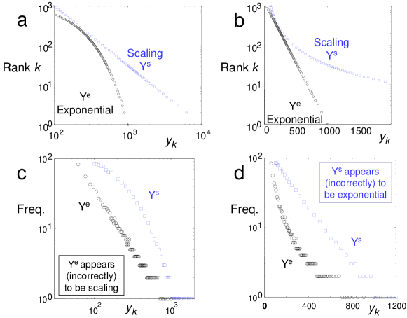
Figure 1: Plots of exponential $y^{e}$ (black circles) and scaling $y^{s}$ (blue squares) sequences. (a) Doubly logarithmic size-rank plot: $y^{s}$ is scaling (to within integer tolerances) and thus $y^{s}_{k}$ versus $k$ is approximately a straight line. (b) Semi-logarithmic size-rank plot:$y^{e}$ is exponential (to within integer tolerances) and thus $y^{e}_{k}$ versus $k$ is approximately a straight line on semi-logarithmic plots (c) Doubly logarithmic size-frequency plot: $y^{e}$ is exponential but appears incorrectly to be scaling (d) Semi-logarithmic size-frequency plot:$y^{s}$ is scaling but appears incorrectly to be exponential.

2.1.3 Cumulative vs. Noncumulative log-log Plots

While in principle there exists an unambiguous mathematical equivalence between distribution functions and their densities, as in (2) and (3), no such relationship can be assumed to hold in general when plotting sequences of real or integer numbers or measured data cumulatively and noncumulatively. Furthermore, there are good practical reasons to avoid noncumulative or size-frequency plots altogether (a sentiment echoed in [75]), even though they are often used exclusively in some communities. To illustrate the basic problem, we first consider two sequences, $y^{s}$ and $y^{e}$, each of length 1000, where $y^{s}=(y^{s}_{1},\ldots,y^{s}_{1000})$ is constructed so that its values all fall on a straight line when plotted on doubly logarithmic (i.e., log-log) scale. Similarly, the values of the sequence $y^{e}=(y^{e}_{1},\ldots,y^{e}_{1000})$ are generated to fall on a straight line when plotted on semi-logarithmic (i.e., log-linear) scale. The matlab code for generating these two sequences is available for electronic download [69]. When ranking the values in each sequence in decreasing order, we obtain the following unique largest (smallest) values, with their corresponding frequencies of occurrence given in parenthesis:

$$y^{s} = \{10000(1),6299(1),4807(1),3968(1),3419(1),\ldots$$

$$\ \ \dots,130(77),121(77),113(81),106(84),100(84)\},$$

$$y^{e} = \{1000(1),903(1),847(1),806(1),775(1),\ldots$$

$$\ \ \dots,96(39),87(43),76(56),61(83),33(180)\},$$

and the full sequences are plotted in Figure 1. In particular, the doubly logarithmic plot in Figure 1(a) shows the cumulative or size-rank relationships associated with the sequences $y^{s}$ and $y^{e}$: the largest value of $y^{s}$ (i.e., 10,000) is plotted on the x-axis and has rank 1 (y-axis), the second largest value of $y^{s}$ is 6,299 and has rank 2, all the way to the end, where the smallest value of $y^{s}$ (i.e., 100) is plotted on the x-axis and has rank 1000 (y-axis). Similarly for $y^{e}$. In full agreement with the underlying generation mechanisms, plotting on doubly logarithmic scale the rank-ordered sequence of $y^{s}$ versus rank $k$ results in a straight line; i.e., $y^{s}$ is scaling (to within integer tolerances). The same plot for the rank-ordered sequence of $y^{e}$ has a pronounced concave shape and decreases rapidly for large ranks—strong evidence for an exponential size-rank relationship. Indeed, as shown in Figure 1(b), plotting on semi-logarithmic scale the rank-ordered sequence of $y^{e}$ versus rank $k$ yields a straight line; i.e., $y^{e}$ is exponential (to within integer tolerances). The same plot for $y^{s}$ shows a pronounced convex shape and decreases very slowly for large rank values—fully consistent with a scaling size-rank relationship. Various metrics for these two sequences are

$$y^{e}$$

(sample) mean 167 267

(sample) median 127 153

(sample) STD 140 504

(sample) CV .84 1.89

and all are consistent with exponential and scaling sequences of this size.

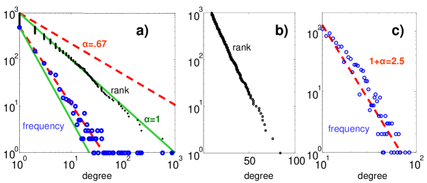
Figure 2: A common error when inferring/estimating scaling behavior. (a) 1000 integer data points sampled from the scaling distribution $P(X\geq x)=x^{-1}$, for $x\geq 1$. The lower size-frequency plot (blue circles) tends to underestimate the scaling index $\alpha$; it supports a slope estimate of about -1.67 (red dashed line), implying an $\alpha$-estimate of about =0.67 that is obviously inconsistent with the true value of $\alpha=1$ (green line). The size-rank plot of the exact same data (upper, black dots) clearly supports a scaling behavior and yields an $\alpha$-estimate that is fully consistent with the true scaling index $\alpha=1$ (green line). (b) 1000 data points sampled from an exponential distribution plotted on log-linear scale. The size-rank plot clearly shows that the data are exponential and that scaling is implausible. (c) The same data as in (b) plotted on log-log scale. Based on the size-frequency plot, it is plausible to infer incorrectly that the data are consistent with scaling behavior, with a slope estimate of about -2.5, implying an $\alpha$-estimate of about 1.5.

To highlight the basic problem caused by the use of noncumulative or size-frequency relationships, consider Figure 1(c) and (d) that show on doubly logarithmic scale and semi-logarithmic scale, respectively, the non-cumulative or size-frequency plots associated with the sequences $y^{s}$ and $y^{e}$: the largest value of $y^{s}$ is plotted on the x-axis and has frequency 1 (y-axis), the second largest value of $y^{s}$ has also frequency 1, etc., until the end where the smallest value of $y^{s}$ happens to occur 84 times (to within integer tolerances). Similarly for $y^{e}$, where the smallest value happens to occur 180 times. It is common to conclude incorrectly from plots such as these, for example, that the sequence $y^{e}$ is scaling (i.e., plotting on doubly logarithmic scale size vs. frequency results in an approximate straight line) and the sequence $y^{s}$ is exponential (i.e., plotting on semi-logarithmic scale size vs. frequency results in an approximate straight line)—exactly the opposite of what is correctly inferred about the sequences using the cumulative or size-rank plots in Figure 1(a) and (b).

In contrast to the size-rank plots of the style in Figure 1(a)-(b) that depict the raw data itself and are unambiguous, the use of size-frequency plots as in Figure 1(c)-(d), while straightforward to describe low variable data, creates ambiguities and can easily lead to mistakes when applied to high variability data. First, for high precision measurements it is possible that each data value appears only once in a sample set, making raw frequency-based data rather uninformative. To overcome this problem, a typical approach is to group individual observations into one of a small number of bins and then plot for each bin (x-axis) the relative number of observations in that bin (y-axis). The problem is that choosing the size and boundary values for each bin is a process generally left up to the experimentalist, and this binning process can dramatically change the nature of the resulting size-frequency plots as well as their interpretation (for a concrete example, see Figure 10 in Section 6.1).

These examples have been artificially constructed specifically to dramatize the effects associated with the use of cumulative or size-rank vs. noncumulative or size-frequency plots for assessing the presence or absence of scaling in given sequence of observed values. While they may appear contrived, errors such as those illustrated in Figure 1 are easy to make and are widespread in the complex systems literature. In fact, determining whether a realization of a sample of size $n$ generated from one and the same (unknown) underlying distribution is consistent with a scaling distribution and then estimating the corresponding tail index $\alpha$ from the corresponding size-frequency plots of the data is even more unreliable. Even under the most idealized circumstances using synthetically generated pseudo-random data, size-frequency plots can mislead as shown in the following easily reproduced numerical experiments. Suppose that 1000 (or more) integer values are generated by pseudo-random independent samples from the distribution $F(x)=1-x^{-1}$ ($P(X\geq x)=x^{-1}$) for $x\geq 1$. For example, this can be done with the matlab fragment x=floor(1./rand(1,1000)) where rand(1,1000) generates a vector of 1000 uniformly distributed floating point numbers between 0 and 1, and floor rounds down to the next lowest integer. In this case, discrete equivalents to equations (2) and (3) exist, and for $x\gg 1$, the density function $f(x)=P[X=x]$ is given by

$$P[X=x] = P[X\geq x]-P[X\geq x+1]$$

$$= x^{-1}-\left({x+1}\right)^{-1}$$

$$\approx x^{-2}.$$

Thus it might appear that the true tail index (i.e., $\alpha=1$) could be inferred from examining either the size-frequency or size-rank plots, but as illustrated in Figure 2 and described in the caption, this is not the case.

Though there are more rigorous and reliable methods for estimating $\alpha$ (see for example [85]), the (cumulative) size-rank plots have significant advantages in that they show the raw data directly, and possible ambiguities in the raw data notwithstanding, they are also highly robust to a range of measurement errors and noise. Moreover, experienced readers can judge at a glance whether a scaling model is plausible, and if so, what a reasonable estimate of the unknown scaling parameter $\alpha$ should be. For example, that the scatter in the data in Figure 2(a) is consistent with a sample from $P(X\geq x)=x^{-1}$ can be roughly determined by visual inspection, although additional statistical tests could be used to establish this more rigorously. At the same time, even when the underlying random variable $X$ is scaling, size-frequency plots systematically underestimate $\alpha$, and worse, have a tendency to suggest that scaling exists where it does not. This is illustrated dramatically in Figure 2(b)-(c), where exponentially distributed samples are generated using floor(10*(1-log(rand(1,n)))). The size-rank plot in Figure 2(b) is approximately a straight line on a semilog plot, consistent with an exponential distribution. The loglog size-frequency plot Figure 2(c) however could be used incorrectly to claim that the data is consistent with a scaling distribution, a surprisingly common error in the SF and broader complex systems literature. Thus even if one a priori assumes a probabilistic framework, (cumulative) size-rank plots are essential for reliably inferring and subsequently studying high variability, and they therefore are used exclusively in this paper.

2.1.4 Scaling: More “normal” than Normal

While power laws in event size statistics in many complex interconnected systems have recently attracted a great deal of popular attention, some of the aspects of scaling distributions that are crucial and important for mathematicians and engineers have been largely ignored in the larger complex systems literature. This subsection will briefly review one aspect of scaling that is particularly revealing in this regard and is a summary of results described in more detail in [67, 111].

Gaussian distributions are universally viewed as “normal”, mainly due to the well-known Central Limit Theorem (CLT). In particular, the ubiquity of Gaussians is largely attributed to the fact that they are invariant and attractors under aggregation of summands, required only to be independent and identically distributed (iid) and have finite variance [47]. Another convenient aspect of Gaussians is that they are completely specified by mean and variance, and the CLT justifies using these statistics whenever their estimates robustly converge, even when the data could not possibly be Gaussian. For example, much data can only take positive values (e.g. connectivity) or have hard upper bounds but can still be treated as Gaussian. It is understood that this approximation would need refinement if additional statistics or tail behaviors are of interest. Exponential distributions have their own set of invariance properties (e.g. conditional expectation) that make them attractive models in some cases. The ease by which Gaussian data is generated by a variety of mechanisms means that the ability of any particular model to reproduce Gaussian data is not counted as evidence that the model represents or explains other processes that yield empirically observed Gaussian phenomena. However, a disconnect often occurs when data have high variability, that is, when variance or coefficient of variation estimates don’t converge. In particular, the above type of reasoning is often misapplied to the explanation of data that are approximately scaling, for reasons that we will discuss below.

Much of science has focused so exclusively on low variability data and Gaussian or exponential models that low variability is not even seen as an assumption. Yet much real world data has extremely high variability as quantified, for example, via the coefficient of variation defined in (5). When exploring stochastic models of high variability data, the most relevant mathematical result is that the CLT has a generalization that relaxes the finite variance (e.g. finite $CV$) assumption, allows for high variability data arising from underlying infinite variance distributions, and yields stable laws in the limit. There is a rich and extensive theory on stable laws (see for example [89]), which we will not attempt to review, but mention only the most important features. Recall that a random variable $U$ is said to have a stable law (with index $0<\alpha\leq 2$) if for any $n\geq 2$, there is a real number $d_{n}$ such that

$$U_{1}+U_{2}+\cdots+U_{n}\stackrel{{\scriptstyle d}}{{=}}n^{1/\alpha}U+d_{n},$$

where $U_{1},~{}U_{2},~{}\ldots,~{}U_{n}$ are independent copies of $U$, and where $\stackrel{{\scriptstyle d}}{{=}}$ denotes equality in distribution. Following [89], the stable laws on the real line can be represented as a four-parameter family $S_{\alpha}(\sigma,\beta,\mu)$, with the index $\alpha$, $0<\alpha\leq 2$; the scale parameter $\sigma>0$; the skewness parameter $\beta$, $-1\leq\beta\leq 1$; and the location (shift) parameter $\mu$, $-\infty<\mu<\infty$. When $1<\alpha<2$, the shift parameter is the mean, but for $\alpha\leq 1$, the mean is infinite. There is an abrupt change in tail behavior of stable laws at the boundary $\alpha=2$. While for $\alpha<2$, all stable laws are scaling in the sense that they satisfy condition (2) and thus exhibit infinite variance or high variability; the case $\alpha=2$ is special and represents a familiar, not scaling distribution—the Gaussian (normal) distribution; i.e., $S_{2}(\sigma,0,\mu)=N(\mu,2\sigma^{2})$, corresponding to the finite variance or low variability case. While with the exception of Gaussian, Cauchy, and Levy distributions, the distributions of stable random variables are not known in closed form, they are known to be the only fixed points of the renormalization group transformation and thus arise naturally in the limit of properly normalized sums of iid scaling random variables. From an unbiased mathematical view, the most salient features of scaling distributions are this and additional strong invariance properties (e.g. to marginalization, mixtures, maximization), and the ease with which scaling is generated by a variety of mechanisms [67, 111]. Combined with the abundant high variability in real world data, these features suggest that scaling distributions are in a sense more “normal” than Gaussians and that they are convenient and parsimonious models for high variability data in as strong a sense as Gaussians or exponentials are for low variability data.

While the ubiquity of scaling is increasingly recognized and even highlighted in the physics and the popular complexity literature [11, 27, 14, 12], the deeper mathematical connections and their rich history in other disciplines have been largely ignored, with serious consequences. Models of complexity using graphs, lattices, cellular automata, and sandpiles preferred in physics and the standard laboratory-scale experiments that inspired these models exhibit scaling only when finely tuned in some way. So even when accepted as ubiquitous, scaling is still treated as arcane and exotic, and “emergence” and “self-organization” are invoked to explain how this tuning might happen [8]. For example, that SF network models supposedly replicate empirically observed scaling node degree relationships that are not easily captured by traditional Erdös-Renyí random graphs [15] is presented as evidence for model validity. But given the strong invariance properties of scaling distributions, as well as the multitude of diverse mechanisms by which scaling can arise in the first place [75], it becomes clear that an ability to generate scaling distributions “explains” little, if anything. Once high variability appears in real data then scaling relationships become a natural outcome of the processes that measure them.

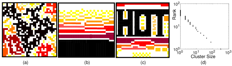
Figure 3: Percolation lattices with scaling cluster sizes. Lattices (a)-(c) have the exact same scaling sequence of cluster sizes (d) and the same (critical) density $\approx.59$). While random lattice such as in (a) have been be called “scale-free”, the highly structured lattices in (b) or (c) typically would not. This suggests that, even within the framework of percolation, scale-free usually means something beyond simple scaling of some statistics and refers to geometric or topological properties.

2.2 Scaling, Scale-free and Self-Similarity

Within the physics community it is common to refer to functions of the form (3) as scale-free because they satisfy the following property

$$f(ax)=g(a)f(x).$$ (6)

As reviewed by Newman [75], the idea is that an increase by a factor $a$ in the scale or units by which one measures $x$ results in no change to the overall density $f(x)$ except for a multiplicative scaling factor. Furthermore, functions consistent with (3) are the only functions that are scale-free in the sense of (6)—free of a characteristic scale. This notion of “scale-free” is clear, and could be taken as simply another synonym for scaling and power law, but most actual usages of “scale-free” appear to have a richer notion in mind, and they attribute additional features, such as some underlying self-similar or fractal geometry or topology, beyond just properties of certain scalar random variables.

One of the most widespread and longstanding uses of the term “scale-free” has been in astrophysics to describe the fractal nature of galaxies. Using a probabilistic framework, one approach is to model the distribution of galaxies as a stationary random process and express clustering in terms of correlations in the distributions of galaxies (see the review [45] for an introduction). In 1977, Groth and Peebles [51] proposed that this distribution of galaxies is well described by a power-law correlation function, and this has since been called scale-free in the astrophysics literature. Scale-free here means that the fluctuation in the galaxy density have “non-trivial, scale-free fractal dimension” and thus scale-free is associated with fractals in the spatial layout of the universe.

Perhaps the most influential and revealing notion of “scale-free” comes from the study of critical phase transitions in physics, where the ubiquity of power laws is often interpreted as a “signature” of a universality in behavior as well in as underlying generating mechanisms. An accessible history of the influence of criticality in the SF literature can found in [14, pp. 73-78]. Here, we will briefly review criticality in the context of percolation, as it illustrates the key issues in a simple and easily visualized way. Percolation problems are a canonical framework in the study of statistical mechanics (see [98] for a comprehensive introduction). A typical problem consists of a square $n\times n$ lattice of “sites”, each of which is either “occupied” or “unoccupied”. This initial configuration is obtained at random, typically according to some uniform probability, termed the density, and changes to the lattice are similarly defined in terms of some stochastic process. The objective is to understand the relationship among groups of contiguously connected sites, called clusters. One celebrated result in the study of such systems is the existence of a phase transition at a critical density of occupied sites, above which there exists with high probability a cluster that spans the entire lattice (termed a percolating cluster) and below which no percolating cluster exists. The existence of a critical density where a percolating cluster “emerges” is qualitatively similar to the appearance of a giant connected component in random graph theory [23].

Figure 3(a) shows an example of a random square lattice ($n=32$) of unoccupied white sites and a critical density ($\approx.59$) of occupied dark sites, shaded to show their connected clusters. As is consistent with percolation problems at criticality, the sequence of cluster sizes is approximately scaling, as seen in Figure 3(d), and thus there is wide variability in cluster sizes. The cluster boundaries are fractal, and in the limit of large $n$, the same fractal geometry occurs throughout the lattice and on all scales, one sense in which the lattice is said to be self-similar and “scale-free”. These scaling, scale-free, and self-similar features occur in random lattices if and only if (with unit probability in the limit of large $n$) the density is at the critical value. Furthermore, at the critical point, cluster sizes and many other quantities of interest have power law distributions, and these are all independent of the details in two important ways. The first and most celebrated is that they are universal, in the sense that they hold identically in a wide variety of otherwise quite different physical phenomena. The other, which is even more important here, is that all these power laws, including the scale-free fractal appearance of the lattice, is unaffected if the sites are randomly rearranged. Such random rewiring preserves the critical density of occupied sites, which is all that matters in purely random lattices.

For many researchers, particularly those unfamiliar with the strong statistical properties of scaling distributions, these remarkable properties of critical phase transitions have become associated with more than just a mechanism giving power laws. Rather, power laws themselves are often viewed as “suggestive” or even “patent signatures” of criticality and “self-organization” in complex systems generally [14]. Furthermore, the concept of Self-Organized Criticality (SOC) has been suggested as a mechanism that automatically tunes the density to the critical point [11]. This has, in turn, given rise to the idea that power laws alone could be “signatures” of specific mechanisms, largely independent of any domain details, and the notion that such phenomena are robust to random rewiring of components or elements has become a compelling force in much of complex systems research.

Our point with these examples is that typical usage of “scale-free” is often associated with some fractal-like geometry, not just macroscopic statistics that are scaling. This distinction can be highlighted through the use of the percolation lattice example, but contrived explicitly to emphasize this distinction. Consider three percolation lattices at the critical density (where the distribution of cluster sizes is known to be scaling) depicted in Figure 3(a)-(c). Even though these lattices have identical cluster size sequences (shown in Figure 3(d)), only the random and fractal, self-similar geometry of the lattice in Figure 3(a) would typically be called “scale-free,” while the other lattices typically would not and do not share any of the other “universal” properties of critical lattices [29]. Again, the usual use of “scale-free” seems to imply certain self-similar or fractal-type features beyond simply following scaling statistics, and this holds in the existing literature on graphs as well.

2.3 Scaling and Self-Similarity in Graphs

While it is possible to use “scale-free” as synonymous with simple scaling relationships as expressed in (6), the popular usage of this term has generally ascribed something additional to its meaning, and the terms “scaling” and “scale-free” have not been used interchangeably, except when explicitly used to say that “scaling” is “free of scale.” When used to describe many naturally occurring and man-made networks, “scale free” often implies something about the spatial, geometric, or topological features of the system of interest (for a recent example of that illustrates this perspective in the context of the World Wide Web, see [38]). While there exists no coherent, consistent literature on this subject, there are some consistencies that we will attempt to capture at least in spirit. Here we review briefly some relevant treatments ranging from the study of river networks to random graphs, and including the study of network motifs in engineering and biology.

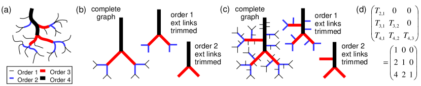
Figure 4: Horton-Strahler streams of order 4. (a) Generic stream with segments coded according to their order. (b) Self-similar tree without side tributaries: branching number $b=2$ and $T_{k}=0$ for all $k$. (c) Self-similar tree with side tributaries: branching number $b=2$ but $T_{k}=2^{k-1}$ for $k=1,2,3$. (d) Toeplitz matrix of values $T_{\omega,\omega-k}=T_{k}$, representing the side tributaries in (c).

2.3.1 Self-similarity of River Channel Networks

One application area where self-similar, fractal-like, and scale-free properties of networks have been considered in great detail has been the study of geometric regularities arising in the analysis of tree-branching structures associated with river or stream channels [53, 101, 52, 68, 60, 82, 106, 39]. Following [82], consider a river network modeled as a tree graph, and recursively assign weights (the “Horton-Strahler stream order numbers”) to each link as follows. First, assign order 1 to all exterior links. Then, for each interior link, determine the highest order among its child links, say, $\omega$. If two or more of the child links have order $\omega$, assign to the parent link order $\omega+1$; otherwise, assign order $\omega$ to the parent link. Order $k$ streams or channels are then defined as contiguous chains of order $k$ links. A tree whose highest order stream has order $\Omega$ is called a tree of order $\Omega$. Using this Horton-Strahler stream ordering concept, any rooted tree naturally decomposes into a discrete set of “scales”, with the exterior links labeled as order 1 streams and representing the smallest scale or the finest level of detail, and the order $\Omega$ stream(s) within the interior representing the largest scale or the structurally coarsest level of detail. For example, consider the order 4 streams and their different “scales” depicted in Figure 4.

To define topologically self-similar trees, consider the class of deterministic trees where every stream of order $\omega$ has $b\geq 2$ upstream tributaries of order $\omega-1$, and $T_{\omega,k}$ side tributaries of order $k$, with $2\leq\omega\leq\Omega$ and $1\leq k\leq\omega-1$. A tree is called (topologically) self-similar if the corresponding matrix $(T_{\omega,k})$ is a Toeplitz matrix; i.e., constant along diagonals, $T_{\omega,\omega-k}=T_{k}$, where $T_{k}$ is a number that depends on $k$ but not on $\omega$ and gives the number of side tributaries of order $\omega-k$. This definition (with the further constraint that $T_{k+1}/T_{k}$ is constant for all $k$) was originally considered in works by Tokunaga (see [82] for references). Examples of self-similar trees of order 4 are presented in Figure 4(b-c).

An important concept underlying this ordering scheme can be described in terms of a recursive “pruning” operation that starts with the removal of the order 1 exterior links. Such removal results in a tree that is more coarse and has its own set of exterior links, now corresponding to the finest level of remaining detail. In the next iteration, these order 2 streams are pruned, and this process continues for a finite number of iterations until only the order $\Omega$ stream remains. As illustrated in Figure 4(b-c), successive pruning is responsible for the self-similar nature of these trees. The idea is that streams of order $k$ are invariant under the operation of pruning—they may be relabeled or removed entirely, but are never severed—and they provide a natural scale or level of detail for studying the overall structure of the tree.

As discussed in [87], early attempts at explaining the striking ubiquity of Horton-Strahler stream ordering was based on a stochastic construction in which “it has been commonly assumed by hydrologists and geomorphologists that the topological arrangement and relative sizes of the streams of a drainage network are just the result of a most probable configuration in a random environment.” However, more recent attempts at explaining this regularity have emphasized an approach based on different principles of optimal energy expenditure to identify the universal mechanisms underlying the evolution of “the scale-free spatial organization of a river network” [87, 86]. The idea is that, in addition to randomness, necessity in the form of different energy expenditure principles play a fundamental role in yielding the multiscaling characteristics in naturally occurring drainage basins.

It is also interesting to note that while considerable attention in the literature on river or stream channel networks is given to empirically observed power law relationships (commonly referred to as “Horton’s laws of drainage network composition”) and their physical explanations, it has been argued in [60, 61, 62] that these “laws” are in fact a very weak test of models or theories of stream network structures. The arguments are based on the observation that because most stream networks (random or non-random) appear to satisfy Horton’s laws automatically, the latter provide little compelling evidence about the forces or processes at work in generating the remarkably regular geometric relationships observed in actual river networks. This discussion is akin to the wide-spread belief in the SF network literature that since SF graphs exhibit power law degree distributions, they are capable of capturing a distinctive “universal” feature underlying the evolution of complex network structures. The arguments provided in the context of the Internet’s physical connectivity structure [65] are similar in spirit to Kirchner’s criticism of the interpretation of Horton’s laws in the literature on river or stream channel networks. In contrast to [60] where Horton’s laws are shown to be poor indicators of whether or not stream channel networks are random, [65] makes it clear that by their very design, engineered networks like the Internet’s router-level topology are essentially non-random, and that their randomly constructed (but otherwise comparable) counterparts result in poorly-performing or dysfunctional networks.

2.3.2 Scaling Degree Sequence and Degree Distribution

Statistical features of graph structures that have received extensive treatment include the size of the largest connected component, link density, node degree relationships, the graph diameter, the characteristic path length, the clustering coefficient, and the betweenness centrality (for a review of these and other metrics see [4, 74, 40]). However, the single feature that has received the most attention is the distribution of node degree and whether or not it follows a power law.

For a graph with $n$ vertices, let $d_{i}={\rm deg}(i)$ denote the degree of node $i$, $1\leq i\leq n$, and call $D=\{d_{1},d_{2},\ldots,d_{n}\}$ the degree sequence of the graph, again assumed without loss of generality always to be ordered $d_{1}\geq d_{2}\geq\ldots\geq d_{n}$. We will say a graph has scaling degree sequence D (or $D$ is scaling) if for all $1\leq k\leq n_{s}\leq n$, $D$ satisfies a power law size-rank relationship of the form $k\ d_{k}^{\alpha}=c$, where $c>0$ and $\alpha>0$ are constants, and where $n_{s}$ determines the range of scaling [67]. Since this definition is simply a graph-specific version of (1) that allows for deviations from the power law relationship for nodes with low connectivity, we again recognize that doubly logarithmic plots of $d_{k}$ versus $k$ yield straight lines of slope $-\alpha$, at least for large $d_{k}$ values.

This description of scaling degree sequence is general, in the sense that it applies to any given graph without regard to how it is generated and without reference to any underlying probability distributions or ensembles. That is, a scaling degree sequence is simply an ordered list of integers representing node connectivity and satisfying the above scaling relationship. In contrast, the SF literature focuses largely on scaling degree distribution, and thus a given degree sequence has the further interpretation as representing a realization of an iid sample of size $n$ generated from a common scaling distribution of the type (2). This in turn is often induced by some random ensemble of graphs. This paper will develop primarily a nonstochastic theory and thus focus on scaling degree sequences, but will clarify the role of stochastic models and distributions as well. In all cases, we will aim to be explicit about which is assumed to hold.

For graphs that are not trees, a first attempt at formally defining and relating the concepts of “scaling” or “scale-free” and “self-similar” through an appropriately defined notion of “scale invariance” is considered by Aiello et al. and described in [3]. In short, Aiello et al. view the evolution of a graph as a random process of growing the graph by adding new nodes and links over time. A model of a given graph evolution process is then called “scale-free” if “coarse-graining” in time yields scaled graphs that have the same power law degree distribution as the original graph. Here “coarse-graining in time” refers to constructing scaled versions of the original graph by dividing time into intervals, combining all nodes born in the same interval into super-nodes, and connecting the resulting super-nodes via a natural mapping of the links in the original graph. For a number of graph growing models, including the Barabási-Albert construction, Aiello et al. show that the evolution process is “scale-free” in the sense of being invariant with respect to time scaling (i.e., the frequency of sampling with respect to the growth rate of the model) and independent of the parameter of the underlying power law node degree distribution (see [3] for details). Note that the scale invariance criterion considered in [3] concerns exclusively the degree distributions of the original graph and its coarse-grained or scaled counterparts. Specifically, the definition of “scale-free” considered by Aiello et al. is not “structural” in the sense that it depends on a macroscopic statistic that is largely uninformative as far as topological properties of the graph are concerned.

2.3.3 Network Motifs

Another recent attempt at relating the notions of “scale-free” and “self-similar” for arbitrary graphs through the more structurally driven concept of “coarse-graining” is due to Itzkovitz et al. [58]. More specifically, the main focus in [58] is on investigating the local structure of basic network building blocks, termed motifs, that recur throughout a network and are claimed to be part of many natural and man-made systems [92, 70]. The idea is that by identifying motifs that appear in a given network at much higher frequencies than in comparable random networks, it is possible to move beyond studying macroscopic statistical features of networks (e.g. power law degree sequences) and try to understand some of the networks’ more microscopic and structural features. The proposed approach is based on simplifying complex network structures by creating appropriately coarse-grained networks in which each node represents an entire pattern (i.e., network motif) in the original network. Recursing on the coarse-graining procedure yields networks at different levels of resolution, and a network is called “scale-free” if the coarse-grained counterparts are “self-similar” in the sense that the same coarse-graining procedure with the same set of network motifs applies at each level of resolution. When applying their approach to an engineered network (electric circuit) and a biological network (protein-signaling network), Itzkovitz et al. found that while each of these networks exhibits well-defined (but different) motifs, their coarse-grained counterparts systematically display very different motifs at each level.

A lesson learned from the work in [58] is that networks that have scaling degree sequences need not have coarse-grained counterparts that are self-similar. This further motivates appropriately narrowing the definition of “scale-free” so that it does imply some kind of self-similarity. In fact, the examples considered in [58] indicate that engineered or biological networks may be the opposite of “scale-free” or “self-similar”—their structure at each level of resolution is different, and the networks are “scale-rich” or “self-dissimilar.” As pointed out in [58], this observation contrasts with prevailing views based on statistical mechanics near phase-transition points which emphasize how self-similarity, scale invariance, and power laws coincide in complex systems. It also suggests that network models that emphasize the latter views may be missing important structural features [58, 59]. A more formal definition of self-dissimilarity was recently given by Wolpert and Macready [112, 113] who proposed it as a characteristic measure of complex systems. Motivated by a data-driven approach, Wolpert and Macready observed that many complex systems tend to exhibit different structural patterns over different space and time scales. Using examples from biological and economic/social systems, their approach is to consider and quantify how such complex systems process information at different scales. Measuring a system’s self-dissimilarity across different scales yields a complexity “signature” of the system at hand. Wolpert and Macready suggest that by clustering such signatures, one obtains a purely data-driven, yet natural, taxonomy for broad classes of complex systems.

2.3.4 Graph Similarity and Data Mining

Finally, the notion of graph similarity is fundamental to the study of attributed graphs (i.e., objects that have an internal structure that is typically modeled with the help of a graph or tree and that is augmented with attribute information). Such graphs arise as natural models for structured data observed in different database applications (e.g., molecular biology, image or document retrieval). The task of extracting relevant or new knowledge from such databases (“data mining”) typically requires some notion of graph similarity and there exists a vast literature dealing with different graph similarity measures or metrics and their properties [91, 31]. However, these measures tend to exploit graph features (e.g., a given one-to-one mapping between the vertices of different graphs, or a requirement that all graphs have to be of the same order) that are specific to the application domain. For example, a common similarity measure for graphs used in the context of pattern recognition is the edit distance [90]. In the field of image retrieval, the similarity of attributed graphs is often measured via the vertex matching distance [83]. The fact that the computation of many of these similarity measures is known to be NP-complete has motivated the development of new and more practical measures that can be used for more efficient similarity searches in large-scale databases (e.g., see [63]).

3 The Existing SF Story

In this section, we first review the existing SF literature describing some of the most popular models and their most appealing features. This is then followed by a brief a critique of the existing theory of SF networks in general and in the context of Internet topology in particular.

3.1 Basic Properties and Claims

The main properties of SF graphs that appear in the existing literature can be summarized as

1. SF networks have scaling (power law) degree distribution.

2. SF networks can be generated by certain random processes, the foremost among which is preferential attachment.

3. SF networks have highly connected “hubs” which “hold the network together” and give the “robust yet fragile” feature of error tolerance but attack vulnerability.

4. SF networks are generic in the sense of being preserved under random degree preserving rewiring.

5. SF networks are self-similar.

6. SF networks are universal in the sense of not depending on domain-specific details.

This variety of features suggest the potential for a rich and extensive theory. Unfortunately, it is unclear from the literature which properties are necessary and/or sufficient to imply the others, and if any implications are strict, or simply “likely” for an ensemble. Many authors apparently define scale-free in terms of just one property, typically scaling degree distribution or random generation, and appear to claim that some or all of the other properties are then consequences. A central aim of this paper is to clarify exactly what options there are in defining SF graphs and deriving their additional properties. Ultimately, we propose below in Section 6.2 a set of minimal axioms that allow for the preservation of the most common claims. However, first we briefly review the existing treatment of the above properties, related historical results, and shortcomings of the current theory, particularly as it has been frequently applied to the Internet.

The ambiguity regarding the definition of “scale-free” originates with the original papers [15, 6], but have continued since. Here SF graphs appear to be defined both as graphs with scaling or power law degree distributions and as being generated by a stochastic construction mechanism based on incremental growth (i.e. nodes are added one at a time) and preferential attachment (i.e. nodes are more likely to attach to nodes that already have many connections). Indeed, the apparent equivalence of scaling degree distribution and preferential attachment, and the ability of thus-defined (if ambiguously so) SF network models to generate node degree statistics that are consistent with the ubiquity of empirically observed power laws is the most commonly cited evidence that SF network mechanisms and structures are in some sense universal [5, 6, 14, 15, 18].

Models of preferential attachment giving rise to power law statistics actually have a long history and are at least 80 years old. As presented by Mandelbrot [67], one early example of research in this area was the work of Yule [117], who in 1925 developed power law models to explain the observed distribution of species within plant genera. Mandelbrot [67] also documents the work of Luria and Delbrück, who in 1943 developed a model and supporting mathematics for the explicit generation of scaling relationships in the number of mutants in old bacterial populations [66]. A more general and popular model of preferential attachment was developed by Simon [94] in 1955 to explain the observed presence of power laws within a variety of fields, including economics (income distributions, city populations), linguistics (word frequencies), and biology (distribution of mutants in bacterial cultures). Substantial controversy and attention surrounded these models in the 1950s and 1960s [67]. A recent review of this history can also be found in [71]. By the 1990s though these models had been largely displaced in the popular science literature by models based on critical phenomena from statistical physics [11], only to resurface recently in the scientific literature in this context of “scale-free networks” [15]. Since then, numerous refinements and modifications to the original Barabási-Albert construction have been proposed and have resulted in SF network models that can reproduce power law degree distributions with any $\alpha\in[1,2]$, a feature that agrees empirically with many observed networks [4]. Moreover, the largely empirical and heuristic studies of these types of “scale-free” networks have recently been enhanced by a rigorous mathematical treatment that can be found in [24] and involves a precise version of the Barabási-Albert construction.

The introduction of SF network models, combined with the equally popular (though less ambiguous) “small world” network models [109], reinvigorated the use of abstract random graph models and their properties (particularly node degree distributions) to study a diversity of complex network systems. For example, Dorogovtsev and Mendes [40, p.76] provide a “standard programme of empirical research of a complex network”, which for the case of undirected graphs consist of finding 1) the degree distribution; 2) the clustering coefficient; 3) the average shortest-path length. The presumption is that these features adequately characterize complex networks. Through the collective efforts of many researchers, this approach has cataloged an impressive list of real application networks, including communication networks (the WWW and the Internet), social networks (author collaborations, movie actors), biological networks (neural networks, metabolic networks, protein networks, ecological and food webs), telephone call graphs, mail networks, power grids and electronic circuits, networks of software components, and energy landscape networks (again, comprehensive reviews of these many results are widely available [4, 14, 74, 40, 79]). While very different in detail, these systems share a common feature in that their degree distributions are all claimed to follow a power law, possibly with different tail indices.

Regardless of the definitional ambiguities, the use of simple stochastic constructions that yield scaling degree distributions and other appealing graph properties represent for many researchers what is arguably an ideal application of statistical physics to explaining and understanding complexity. Since SF models have their roots in statistical physics, a key assumption is always that any particular network is simply a realization from a larger ensemble of graphs, with an explicit or implicit underlying stochastic model. Accordingly, this approach to understanding complex networks has focused on those networks that are most likely to occur under an assumed random graph model and has aimed at identifying or discovering macroscopic features that capture the “essence” of the structure underlying those networks. Thus preferential attachment offers a general and hence attractive “microscopic” mechanism by which a growth process yields an ensemble of graphs with the “macroscopic” property of power law node degree distributions [16]. Second, the resulting SF topologies are “generic.” Not only is any specific SF graph the generic or likely element from such an ensemble, but also “… an important property of scale-free networks is that [degree preserving] random rewiring does not change the scale-free nature of the network” (see Methods Supplement to [55]). Finally, this ensemble-based approach has an appealing kind of “universality” in that it involves no model-specific domain knowledge or specialized “design” requirements and requires only minimal tuning of the underlying model parameters.

Perhaps most importantly, SF graphs are claimed to exhibit a host of startling “emergent” consequences of universal relevance, including intriguing self-similar and fractal properties (see below for details), small-world characteristics [9], and “hub-like” cores. Perhaps the central claim for SF graphs is that they have hubs, what we term SF hubs, which “hold the network together.” As noted, the structure of such networks is highly vulnerable (i.e., can be fragmented) to attacks that target these hubs [6]. At the same time, they are resilient to attacks that knock out nodes at random, since a randomly chosen node is unlikely to be a hub and thus its removal has minimal effect on network connectivity. In the context of the Internet, where SF graphs have been proposed as models of the router-level Internet [115], this has been touted “the Achilles’ heel of the Internet” [6], a vulnerability that has presumably been overlooked by networking engineers. Furthermore, the hub-like structure of SF graphs is such that the epidemic threshold is zero for contagion phenomena [78, 13, 80, 79], thus suggesting that the natural way to stop epidemics, either for computer viruses/worms or biological epidemics such as AIDS, is to protect these hubs [37, 26]. Proponents of this modeling framework have further suggested that the emergent properties of SF graphs contributes to truly universal behavior in complex networks [22] and that preferential attachment as well is a universal mechanism at work in the evolution of these networks [56, 40].

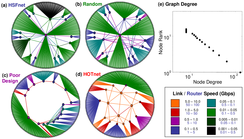
Figure 5: Network graphs having exactly the same number of nodes and links, as well as the same (power law) degree sequence. As toy models of the router-level Internet, all graphs are subject to same router technology constraints and the same traffic demand model for routers at the network periphery. (a) Hierarchical scale-free (HSF) network: Following roughly a recently proposed construction that combines scale-free structure and inherent modularity in the sense of exhibiting an hierarchical architecture [84], we start with a small 3-pronged cluster and build a 3-tier network a la Ravasz-Barabási, adding routers at the periphery roughly in a preferential manner. (b) Random network: This network is obtained from the HSF network in (a) by performing a number of pairwise random degree-preserving rewiring steps. (c) Poor design: In this heuristic construction, we arrange the interior routers in a line, pick a node towards the middle to be the high-degree, low bandwidth bottleneck, and establish connections between high-degree and low-degree nodes. (d) HOT network: The construction mimics the build-out of a network by a hypothetical ISP. It produces a 3-tier network hierarchy in which the high-bandwidth, low-connectivity routers live in the network core while routers with low-bandwidth and high-connectivity reside at the periphery of the network. (e) Node degree sequence for each network. Only $d_{i}>1$ shown.

3.2 A Critique of Existing Theory

The SF story has successfully captured the interest and imagination of researchers across disciplines, and with good reason, as the proposed properties are rich and varied. Yet the existing ambiguity in its mathematical formulation and many of its most essential properties has created confusion about what it means for a network to be “scale-free” [48]. One possible and apparently popular interpretation is that scale-free means simply graphs with scaling degree sequences, and that this alone implies all other features listed above. We will show that this is incorrect, and in fact none of the features follows from scaling alone. Even relaxing this to random graphs with scaling degree distributions is by itself inadequate to imply any further properties. A central aim of this paper is to clarify the reasons why these interpretations are incorrect, and propose minimal changes to fix them. The opposite extreme interpretation is that scale-free graphs are defined as having all of the above-listed properties. We will show that this is possible in the sense that the set of such graphs is not empty, but as a definition this leads to two further problems. Mathematically, one would prefer fewer axioms, and we will rectify this with a minimal definition. We will introduce a structural metric that provides a view of the extent to which a graph is scale-free and from which all the above properties follow, often with necessary and sufficient conditions. The other problem is that the canonical examples of apparent SF networks, the Internet and biological metabolism, are then very far from scale-free in that they have none of the above properties except perhaps for scaling degree distributions. This is simply an unavoidable conflict between these properties and the specifics of the applications, and cannot be fixed.

As a result, a rigorous theory of SF graphs must either define scale-free more narrowly than scaling degree sequences or distributions in order to have nontrivial emergent properties, and thus lose central claims of applicability, or instead define scale-free as merely scaling, but lose all the universal emergent features that have been claimed to hold for SF networks. We will pursue the former approach because we believe it is most representative of the spirit of previous studies and also because it is most inclusive of results in the existing literature. At the most basic level, simply to be a nontrivial and novel concept, scale-free clearly must mean more than a graph with scaling degree sequence or distribution. It must capture some aspect of the graph itself, and not merely a sequence of integers, stochastic or not, in which case the SF literature and this paper would offer nothing new. Other authors may ultimate choose different definitions, but in any case, the results in this paper clarify for the first time precisely what the graph theoretic alternatives are regarding the implications of any of the possible alternative definitions. Thus the definition of the word “scale-free” is much less important than the mathematical relationship between their various claimed properties, and the connections with real world networks.

3.3 The Internet as a Case Study

To illustrate some key points about the existing claims regarding SF networks as adopted in the popular literature and their relationship with scaling degree distributions, we consider an application to the Internet where graphs are meant to model Internet connectivity at the router-level. For a meaningful explanation of empirically observed network statistics, we must account for network design issues concerned with technology constraints, economic factors, and network performance [65, 41]. Additionally, we should annotate the nodes and links in connectivity-only graphs with domain-specific information such as router capacity and link bandwidth in such a way that the resulting annotated graphs represent technically realizable and functional networks.

3.3.1 The SF Internet

Consider the simple toy model of a “hierarchical” SF network HSFnet shown in Figure 5(a), which has a “modular” graph constructed according to a particular type of preferential attachment [84] and to which are then preferentially added degree-one end systems, yielding the power law degree sequence shown in Figure 5(e). This type of construction has been suggested as a SF model of both the Internet and biology, both of which are highly hierarchical and modular [18]. The resulting graph has all the features listed above as characteristic of SF networks and is easily visualized and thus convenient for our comparisons. Note that the highest-degree nodes in the tail of the degree sequence in Figure 5(e) correspond to the SF hub nodes in the SF network HSFnet, Figure 5(a). This confirms the intuition behind the popular SF view that power law degree sequences imply the existence of SF hubs that are crucial for global connectivity. If such features were true for the real Internet, this finding would certainly be startling and profound, as it directly contradicts the Internet’s legendary and most clearly understood robustness property, i.e., it’s high resilience to router failures [33].

Figure 5 also depicts three other networks with the exact same degree sequence as HSFnet. The variety of these graphs suggests that the set of all connected simple graphs (i.e., no self-loops or parallel links) having exactly the same degree sequence shown in Figure 5(e) is so diverse that its elements appear to have nothing in common as graphs beyond what trivially follows from having a fixed (scaling) degree sequence. They certainly do not appear to share any of the features summarized above as conventionally claimed for SF graphs. Even more striking are the differences in their structures and annotated bandwidths (i.e., color-coding of links and nodes in Figure 5). For example, while the graphs in Figure 5(a) and (b) exhibit the type of hub nodes typically associated with SF networks, the graph in Figure 5(d) has its highest-degree nodes located at the networks’ peripheries. We will show this provides concrete counterexamples to the idea that power law degree sequences imply the existence of SF hubs. This then creates the obvious dilemma as to the concise meaning of a “scale-free graph” as outlined above.

3.3.2 A Toy Model of the Real Internet

In terms of using SF networks as models for the Internet’s router-level topology, recent Internet research has demonstrated that the real Internet is nothing like Figure 5(a), size issues notwithstanding, but is at least qualitatively more like the network shown in Figure 5(d). We label this network HOTnet (for Heuristically Optimal Topology), and note that its overall power law in degree sequence comes from high-degree routers at the network periphery that aggregate the traffic of end users having low bandwidth demands, while supporting aggregate traffic flows with a mesh of low-degree core routers [65]. In fact, as we will discuss in greater detail in Section 6, there is little evidence that the Internet as a whole has scaling degree or even high variability, and much evidence to the contrary, for many of the existing claims of scaling are based on a combination of relying on highly ambiguous data and making a number of statistical errors, some of them similar to those illustrated in Figures 1 and 2. What is true is that a network like HOTnet is consistent with existing technology, and could in principle be the router level graph for some small but plausible network. Thus a network with a scaling degree sequence in its router graph is plausible even if the actual Internet is not scaling. It would however look qualitatively like HOTnet and nothing like HSFnet.

To see in what sense HOTnet is heuristically optimal, note that from a network design perspective, an important question is how well a particular topology is able to carry a given demand for traffic, while fully complying with actual technology constraints and economic factors. Here, we adopt as standard metric for network performance the maximum throughput of the network under a “gravity model” of end user traffic demands [118]. The latter assumes that every end node $i$ has a total bandwidth demand $x_{i}$, that two-way traffic is exchanged between all pairs $(i,j)$ of end nodes $i$ and $j$, the flow $X_{ij}$ of traffic between $i$ and $j$ is given by $X_{ij}=\rho x_{i}x_{j}$, where $\rho$ is some global constant, and is otherwise uncorrelated from all other flows. Our performance measure for a given network $g$ is then its maximum throughput with gravity flows, computed as

$$\mbox{\em Perf}(g)={\max_{\rho}\sum_{ij}X_{ij}},~{}~{}~{}s.t.~{}RX\leq B,$$ (7)

where $R$ is the routing matrix obtained using standard shortest path routing. $R=[R_{kl}]$, with $R_{kl}=1$ if flow $l$ passes through router $k$, and $R_{kl}=0$ otherwise. $X$ is the vector of all flows $X_{ij}$, indexed to match the routing matrix $R$, and $B$ is a vector consisting of all router bandwidth capacities.

An appropriate treatment of router bandwidth capacities represented in $B$ is important for computing network performance and merits additional explanation. Due to fundamental limits in technology, routers must adhere to flow conservation constraints in the total amount of traffic that they process per unit of time. Thus, routers can support a large number of low bandwidth connections or a smaller number of high bandwidth connections. In many cases, additional routing overhead actually causes the total router throughput to decrease as the number of connections gets large, and we follow the presentation in [65] in choosing the term $B$ to correspond with an abstracted version of a widely deployed Cisco product (for details about this abstracted constraint and the factors affecting real router design, we refer the reader to [7, 65]).

The application of this network performance metric to the four graphs in Figure 5 shows that although they have the same degree sequence, they are very different from the perspective of network engineering, and that these differences are significant and critical. For example, the SF network HSFnet in Figure 5(a) achieves a performance of $\mbox{\em Perf}(HSFnet)=6.17\times 10^{8}$ bps, while the HOT network HOTnet in Figure 5(d) achieves a performance of $\mbox{\em Perf}(HOTnet)=2.93\times 10^{11}$ bps, which is greater by more than two orders of magnitude. The reason for this vast difference is that the HOT construction explicitly incorporates the tradeoffs between realistic router capacities and economic considerations in its design process while the SF counterpart does not.

The actual construction of HOTnet is fairly straightforward, and while it has high performance, it is not formally optimal. We imposed the constraints that it must have exactly the same degree sequence as HSFnet, and that it must satisfy the router degree/bandwidth constraints. For a graph of this size the design then easily follows by inspection, and mimics in a highly abstracted way the design of real networks. First, the degree one nodes are designated as end-user hosts and placed at the periphery of the network, though geography per se is not explicitly considered in the design. These are then maximally aggregated by attaching them to the highest degree nodes at the next level in from the periphery, leaving one or two links on these “access router” nodes to attach to the core. The lowest degree of these access routers are given two links to the core, which reflects that low degree access routers are capable of handling higher bandwidth hosts, and such high value customers would likely have multiple connections to the core. At this point there are just 4 low degree nodes left, and these become the highest bandwidth core routers, and are connected in a mesh, resulting in the graph in Figure 5(d). While some rearrangements are possible, all high performance networks using a gravity model and the simple router constraints we have imposed would necessarily look essentially like HOTnet. They would all have the highest degree nodes connected to degree one nodes at the periphery, and they would all have a low-degree mesh-like core.

Another feature that has been highlighted in the SF literature is the attack vulnerability of high degree hubs. Here again, the four graphs in Figure 5 are illustrative of the potential differences between graphs having the same degree sequence. Using the performance metric defined in (7), we compute the performance of each graph without disruption (i.e., the complete graph), after the loss of high degree nodes, and after the loss of the most important (i.e., worst case) nodes. In each case, when removing a node we also remove any corresponding degree-one end-hosts that also become disconnected, and we compute performance over shortest path routes between remaining nodes but in a manner that allows for rerouting. We find that for HSFnet, removal of the highest degree nodes does in fact disconnect the network as a whole, and this is equivalent to the worst case attack for this network. In contrast, removal of the highest degree nodes results in only minor disruption to HOTnet, but a worst case attack (here, this is the removal of the low-degree core routers) does disconnect the network. The results are summarized below.

Network	Complete	High Degree	Worst Case
Performance	Graph	Nodes Removed	Nodes Removed
HSFnet	$5.9197e+09$	Disconnected	= ‘High Degree’ case
HOTnet	$2.9680e+11$	$2.7429e+11$	Disconnected

This example thus illustrates two important points. The first is that HSFnet does indeed have all the graph theoretic properties listed above that are attributed to SF networks, including attack vulnerability, while HOTnet has none of these features except for scaling degree. Thus the set of graphs that have the standard scale-free attributes is neither empty nor trivially equivalent to graphs having scaling degree. The second point is that the standard SF models are in all important ways exactly the opposite of the real Internet, and fail to capture even the most basic features of the Internet’s router-level connectivity. While the intuition behind these claims is clear from inspection of Figure 5 and the performance comparisons, full clarification of these points requires the results in the rest of this paper and additional details on the Internet [7, 65, 41]. These observations naturally cast doubts on the relevance of conventional SF models in other application areas where domain knowledge and specific functional requirements play a similarly crucial role as in the Internet context. The other most cited SF example is metabolic networks in biology, where many recent SF studies have focused on abstract graphs in which nodes represent metabolites, and two nodes are “connected” if they are involved in the same reaction. In these studies, observed power laws for the degree sequences associated with such graphs have been used to claim that metabolic networks are scale-free [19]. Though the details are far more complicated here than in the Internet story above, recent work in [102] that is summarized in Section 7 has shown there is a largely parallel story in that the SF claims are completely inconsistent with the actual biology, despite their superficial appeal and apparent popularity.

4 A Structural Approach

In this section, we show that considerable insight into the features of SF graphs and models is available from a metric that measures the extent to which high-degree nodes connect to other high-degree nodes. As we will show, such a metric is both necessary and useful for explaining the extreme differences between networks that have identical degree sequence, especially if it is scaling. By focusing on a graph’s structural properties and not on not how it was generated, this approach does not depend on an underlying random graph model but is applicable to any graph of interest.

4.1 The $s$-Metric

Let $g$ be an undirected, simple, connected graph having $n=|\mathcal{V}|$ nodes and $l=|\mathcal{E}|$ links, where $\mathcal{V}$ and $\mathcal{E}$ are the sets of nodes and links, respectively. As before, define $d_{i}$ to be the degree of node $i\in\mathcal{V}$, $D=\{d_{1},d_{2},\dots,d_{n}\}$ to be the degree sequence for $g$ (again assumed to be ordered), and let $G(D)$ denote the set of all connected simple graphs having the same degree sequence $D$. Note that most graphs with scaling degree will be neither simple nor connected, so this is an important and nontrivial restriction. Even with these constraints, it is clear based on the previous examples that the elements of $G(D)$ can be very different from one another, so that in order to constitute a non-trivial concept, “scale-free” should mean more than merely that $D$ is scaling and should depend on additional topological or structural properties of the elements in $G(D)$.

Definition 1.

For any graph $g$ having fixed degree sequence $D$, we define the metric

$$s(g)=\sum_{(i,j)\in\mathcal{E}}d_{i}d_{j}.$$ (8)

Note that $s(g)$ depends only on the graph $g$ and not explicitly on the process by which it is constructed. Implicitly, the metric $s(g)$ measures the extent to which the graph $g$ has a “hub-like” core and is maximized when high-degree nodes are connected to other high-degree nodes. This observation follows from the Rearrangement Inequality [114], which states that if $a_{1}\geq a_{2}\geq\cdots\geq a_{n}$ and $b_{1}\geq b_{2}\geq\cdots\geq b_{n}$, then for any permutation $(a^{\prime}_{1},a^{\prime}_{2},\cdots,a^{\prime}_{n})$ of $(a_{1},a_{2},\cdots,a_{n})$, we have

$$a_{1}b_{1}+a_{2}b_{2}+\cdots+a_{n}b_{n} \geq a^{\prime}_{1}b_{1}+a^{\prime}_{2}b_{2}+\cdots+a^{\prime}_{n}b_{n}$$

$$\geq a_{n}b_{1}+a_{n-1}b_{2}+\cdots+a_{1}b_{n}.$$

Since high $s(g)$-values are achieved only by connecting high-degree nodes to each other, and low $s(g)$-values are obtained by connecting high-degree nodes only to low-degree nodes, the $s$-metric moves beyond simple statements concerning the presence of “hub” nodes (as is true for any degree sequence $D$ that has high variability) and attempts to quantify what role such hubs play in the overall structure of the graph. In particular, as we will show below, graphs with relatively high $s(g)$ values have a “hub-like core” in the sense that these hubs play a central role in the overall connectivity of the network. We will also demonstrate that the metric $s(g)$ provides a view that is not only mathematically convenient and rigorous, but also practically useful as far as what it means for a graph to be “scale-free”.

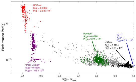
Figure 6: Exploration of the space of connected network graphs having exactly the same (power law) degree sequence. Values for the four networks are shown together with the values for other networks obtained by pairwise degree-preserving rewiring. Networks that are “one-rewiring” away from their starting point are shown in a corresponding color, while other networks obtained from more than one rewiring are shown in gray. Ultimately, only a careful design process explicitly incorporating technological constraints, traffic demands, or link costs yields high-performance networks. In contrast, equivalent networks resulting from even carefully crafted random constructions result in poor-performing networks.

4.1.1 Graph Diversity and the $\mbox{\em Perf}(g)$ vs. $s(g)$ Plane

Although our interest in this paper will be in graphs for which the degree sequence $D$ is scaling, we can compute $s(g)$ with respect to any “background” set $G$ of graphs, and we need not restrict the set to scaling or even to connected or simple graphs. Moreover, for any background set, there exists a graph whose connectivity maximizes the $s$-metric defined in (8), and we refer to this as an “$s_{\max}$ graph”. The $s_{\max}$ graphs for different background sets are of interest since they are essentially unique and also have the most “hub-like” core structure. Graphs with low $s$-values are also highly relevant, but unlike $s_{\max}$ graphs they are extremely diverse with essentially no features in common with each other or with other graphs in the background set except the degree sequence $D$.

Graphs with high variability and/or scaling in their degree sequence are of particular interest, however, and not simply because of their association with SF models. Intuitively, scaling degrees appear to create great “diversity” in $G(D)$. Certainly the graphs in Figure 5 are extremely diverse, despite having identical scaling degree $D$, but to what extent does this depend on $D$ being scaling? As a partial answer, note that at the extremes of variability are $m$-regular graphs with $CV(D)=0$, which have $D=\{m,m,m,\ldots,m\}$ for some $m$, and perfect star-like graphs with $D=\{n-1,1,1,1,\ldots,1\}$, which have maximal $CV(D)\approx\sqrt{n}/2$. In both of these extremes all graphs in $G(D)$ are isomorphic and thus have only one value of $s(g)$ for all $g\in G(D)$ so from this measure the space $G(D)$ of graphs lacks any diversity. In contrast, when $D$ is scaling with $\alpha<2$, $CV(D)\rightarrow\infty$ and it is easy to construct $g$ such that $s(g)/s_{\max}\rightarrow 0$ as $n\rightarrow\infty$, suggesting a possibly enormous diversity in $G(D)$.

Before proceeding with a discussion of some of the features of the $s$-metric as well as for graphs having high $s(g)$ values, we revisit the four toy networks in Figure 5 and consider the combined implications of the performance-oriented metric $\mbox{\em Perf}(g)$ introduced in (7) and the connectivity-specific metric $s(g)$ defined above. Figure 6 is a projection of $g\in G(D)$ onto a plane of $\mbox{\em Perf}(g)$ versus $s(g)$ and will be useful throughout in visualizing the extreme diversity in the set $G(D)$ for $D$ in Figure 5. Of relevance to the Internet application is that graphs with high $s(g)$-values tend to have low performance, although a low $s(g)$-value is no guarantee of good performance, as seen by the network in Figure 5(c) which has both small $s(g)$ and small $\mbox{\em Perf}(g)$. The additional points in the $\mbox{\em Perf}(g)$ vs. $s(g)$ plane involve degree preserving rewiring and will be discussed in more detail below.

These observations undermine the claims in the SF literature that are based on scaling degree alone implying any additional graph properties. On the other hand, they also suggest that the sheer diversity of $G(D)$ for scaling $D$ makes it an interesting object of study. We won’t further compare $G(D)$ for scaling versus non-scaling $D$ or attempt to define “diversity” precisely here, though these are clearly interesting topics. We will focus on exploring the nature of the diversity of $G(D)$ for scaling $D$ such as in Figure 5.

In what follows, we will provide evidence that graphs with high $s(g)$ enjoy certain self-similarity properties, and we also consider the effects of random degree-preserving rewiring on $s(g)$. In so doing, we argue that the $s$-metric, as well as many of the other definitions and properties that we will present, are of interest for any graph or any set of graphs. However, we will continue to focus our attention primarily on simple connected graphs having scaling degree sequences. The main reason is that many applications naturally have simple connected graphs. For example, while the Internet protocols in principle allow router connectivity to be nonsimple, it is relatively rare and has little impact on network properties. Nevertheless, using other sets in many cases is preferable and will arise naturally in the sequel. Furthermore, while our interest will be on simple, connected graphs with scaling degree sequence, we will often specialize our presentation to trees, in order to simplify the development and maximize contact with the existing SF literature. To this end, we will exploit the construction of the $s_{\max}$ graph to sketch some of these relationships in more detail.

4.1.2 The $s_{\max}$ Graph and Preferential Attachment

Given a particular degree sequence $D$, it is possible to construct the $s_{\max}$ graph of $G(D)$ using a deterministic procedure, and both the generation process and its resulting structure are informative about the $s(g)$ metric. Here, we describe this construction at a high level of abstraction (with all details deferred to Appendix A) in order to provide appropriate context for the discussion of key features that is to follow.

The basic idea for constructing the $s_{\max}$ graph is to order all potential links $(i,j)$ for all $i,j\in\mathcal{V}$ according to their weight $d_{i}d_{j}$ and then add them one at a time in a manner that results in a simple, connected graph having degree sequence $D$. While simple enough in concept, this type of “greedy” heuristic procedure may have difficulty achieving the intended sequence $D$ due to the global constraints imposed by connectivity requirements. While the specific conditions under which this procedure is guaranteed to yield the $s_{\max}$ graph are deferred to Appendix A, we note that this type of construction works well in practice for the networks under consideration in this paper, particularly those in Figure 5.

In cases where the intended degree sequence $D$ satisfies $\sum_{i}d_{i}=2(n-1)$, then all simple connected graphs having degree sequence $D$ correspond to trees (i.e., acyclic graphs), and this simple construction procedure is guaranteed to result in an $s_{\max}$ graph. Acyclic $s_{\max}$ graphs have several nice properties that we will exploit throughout this presentation. It is worth noting that since adding links to a tree is equivalent to adding nodes one at a time, construction of acyclic $s_{\max}$ graphs can be viewed essentially as a type of deterministic preferential attachment. Perhaps more importantly, by its construction the $s_{\max}$ tree has a natural ordering within its overall structure, which we now summarize.

Recall that a tree can be organized into hierarchies by designating a single vertex as the “root” of the tree from which all branches emanate. This is equivalent to assigning a direction to each arc such that all arcs flow away from the root. As a result, each vertex of the graph becomes naturally associated with a particular “level” of the hierarchy, adjacent vertices are separated by a single level, and the position of a vertex within the hierarchy is in relation to the root. For example, assuming the root of the tree is at level 0 (the “highest” level), then its neighbors are at level 1 (“below” level 0), their other neighbors in turn are at level 2 (“below” level 1), and so on.

Mathematically, the choice of the root vertex is an arbitrary one, however for the $s_{\max}$ tree, the vertex with largest degree sits as the natural root and is the most “central” (a notion we will formalize below). With this selection, two vertices $u,v\in\mathcal{V}$ that are directly connected to each other in the acyclic $s_{\max}$ graph have the following relative position within the hierarchy. If $d_{u}\geq d_{v}$, then vertex $u$ is one level “above” vertex $v$ (alternatively, we say that vertex $u$ is “upstream” of vertex $v$ or that vertex $v$ is “downstream” from vertex $u$). Thus, moving up the hierarchy of the tree (i.e., upstream) means that vertex degrees are (eventually) becoming larger, and moving down the hierarchy (i.e., downstream) means that vertex degrees are (eventually) becoming smaller.

In order to illustrate this natural ordering within the $s_{\max}$ tree, we introduce the following notation. For any vertex $v\in\mathcal{V}$, let $\mathcal{N}(v)$ denote the set of neighboring vertices for $v$, where for simple connected graphs $|\mathcal{N}(v)|=d_{v}$. For an acyclic graph $g$, define $\tilde{g}^{(v)}$ to be the subgraph (subtree) of vertex $v$; that is, $\tilde{g}^{(v)}$ is the subtree containing vertex $v$ along with all downstream nodes. Since the notion of upstream/downstream is relative to the overall root of the graph, for convenience we will additionally use the notation $\tilde{g}^{(v,u)}$ to represent the subgraph of the vertex $v$ that is itself connected to upstream neighbor vertex $u$. The (ordered) degree sequence of the subtree $\tilde{g}^{(v)}$ (equivalently for $\tilde{g}^{(v,u)}$) is then $D(\tilde{g}^{(v)})=\{d^{(v)}_{1},d^{(v)}_{2},\dots\}$, where $d^{(v)}_{1}=d_{v}$ and the rest of the sequence represents the degrees of all downstream nodes. $D(\tilde{g}^{(v)})$ is clearly a subsequence of $D(g)$. Finally, let $\mathcal{E}(\tilde{g}^{(v)})$ denote the set of edges in the subtree $\tilde{g}^{(v)}$.

For this subtree, we define its $s$-value as

$$s(\tilde{g}^{(v,u)}) = d_{v}d_{u}+\sum_{(j,k)\in\mathcal{E}(\tilde{g}^{(v)})}d_{j}d_{k}.$$ (9)

This definition provides a natural decomposition for the $s$-metric, in that for any vertex $v\in\mathcal{V}$, we can write

$$s(g)=\sum_{k\in\mathcal{N}(v)}s(\tilde{g}^{(k,v)}).$$

Furthermore, the $s$-value for any subtree can be defined as a recursive relationship on its downstream subtrees, specifically

$$s(\tilde{g}^{(v,u)}) = d_{v}d_{u}+\sum_{k\in\mathcal{N}(v)\backslash u}s(\tilde{g}^{(k,v)}).$$

Proposition 1.

Let $g$ be the $s_{\max}$ acyclic graph corresponding to degree sequence $D$. Then for two vertices $u,v\in\mathcal{V}$ with $d_{u}>d_{v}$ it necessarily follows that

1. vertex $v$ cannot be upstream from vertex $u$;

2. the number of vertices in $\tilde{g}^{(v)}$ cannot be greater than the number of vertices in $\tilde{g}^{(u)}$ (i.e., $|D(\tilde{g}^{(u)})|\geq|D(\tilde{g}^{(v)})|$);

3. the degree sequence of $\tilde{g}^{(u)}$ dominates that of $\tilde{g}^{(v)}$ (i.e., $d^{(u)}_{1}\geq d^{(v)}_{1},d^{(u)}_{2}\geq d^{(v)}_{2},\dots$); and

4. $s(\tilde{g}^{(u)})>s(\tilde{g}^{(v)})$.

Although we do not prove each of these statements formally, each of parts (a)-(d) is true by simple contradiction. Essentially, if any of these statements is false, there is a rewiring operation that can be performed on the graph $g$ that increases its $s$-value, thereby violating the assumption that $g$ is the $s_{\max}$ graph. See Appendix A for additional information.

Proposition 2.

Let $g$ be the $s_{\max}$ acyclic graph corresponding to degree sequence $D$. Then it necessarily follows that for each $v\in\mathcal{V}$ and any $k\neq v\in\mathcal{V}$, the subgraph $\tilde{g}^{(v)}$ maximizes $s(g^{(v,k)})$ for the degree sequence $D(\tilde{g}^{(v)})$.

The proof of Proposition 2 follows from an inductive argument that starts with the leaves of the tree and works its way upstream. Essentially, in order for a tree to be the $s_{\max}$ acyclic graph, then each of its branches must be the $s_{\max}$ subtree on the corresponding degree subsequence, and this must hold at all levels of the hierarchy.

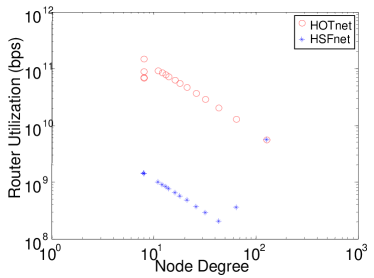
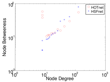
Figure 7: Left: The centrality of nodes as defined by total traffic throughput. The most “central” nodes in HOTnet are the low-degree core routers while the most “central” node in HSFnet is the highest-degree “hub”. The HOTnet throughputs are close to the router bandwidth constraints. Right: The betweenness centrality versus node degree for non-degree-one nodes from both the HSFnet and HOTnet graphs in Figure 5. In HSFnet, node centrality increases with node degree, and the highest degree nodes are the most “central”. In contrast, many of the most “central” nodes in HOTnet have low degree, and the highest degree nodes are significantly less “central” than in HSFnet.

4.2 The $s$-Metric and Node Centrality

While considerable attention has been devoted to network node degree sequences in order to measure the structure of complex networks, it is clear that such sequences alone are insufficient to characterize the aggregate structure of a graph. Figure 5 has shown that high degree nodes can exist at the periphery of the network or at its core, with serious consequences for issues such as network performance and robustness in the presence of node loss. At the same time, it is clear from the $s_{\max}$ construction procedure that graphs with the largest $s(g)$ values will have their highest degree nodes located in the network core. Thus, an important question relates to the centrality of individual high-degree nodes within the larger network and how this relates, if at all, to the $s$-metric for graph structure. Again, the answer to this question helps to quantify the role that individual “hub” nodes play in the overall structure of a network.

There are several possible means for measuring node centrality, and in the context of the Internet, one such measure is the total throughput (or utilization) of a node when the network supports its maximum flow as defined in (7). The idea is that under a gravity model in which traffic demand occurs between all node pairs, nodes that are highly utilized are central to the overall ability of the network to carry traffic. Figure 7 shows the utilization of individual nodes within HSFnet and HOTnet, when each network supports its respective maximum flow, along with the corresponding degree for each node. The picture for HOTnet illustrates that the most “central” nodes are in fact low-degree nodes, which correspond to the core routers in Figure 5(c). In contrast, the node with highest utilization in HSFnet is the highest degree node, corresponding to the “central hub” in Figure 5(a).

Another, more graph theoretic, measure of node centrality is its so-called betweenness (also known as betweenness centrality), which is most often calculated as the fraction of shortest paths between node pairs that pass through the node of interest [40]. Define $\sigma_{st}$ to be the number of shortest paths between two nodes $s$ and $t$. Then, the betweenness centrality of any vertex $v$ can be computed as

$$C_{b}(v)=\frac{\sum_{s<t\in\mathcal{V}}\sigma_{st}(v)}{\sum_{s<t\in\mathcal{V}}\sigma_{st}},$$

where $\sigma_{st}(v)$ is the number of paths between $s$ and $t$ that pass through node $v$. In this manner, betweenness centrality provides a measure of the traffic load that a node must handle. An alternate interpretation is that it measures the influence that an individual node has in the spread of information within the network.

Newman [72] introduces a more general measure of betweenness centrality that includes the flow along all paths (not just the shortest ones), and based on an approach using random walks demonstrates how this quantity can be computed by matrix methods. Applying this alternate metric from [72] to the simple annotated graphs in Figure 5, we observe in Figure 7 that the high-degree nodes in HSFnet are the most central, and in fact this measure of betweeness centrality increases with node degree. In contrast, most of the nodes in HOTnet that are central are not high degree nodes, but the low-degree core routers.

Understanding the betweenness centrality of individual nodes is considerably simpler in the context of trees. Recall that in an acyclic graph there is exactly one path between any two vertices, making the calculation of $C_{b}(v)$ rather straightforward. Specifically, observe that $\sum_{s<t\in\mathcal{V}}\sigma_{st}=n(n-1)/2$ and that for each $s\neq v\neq t\in\mathcal{V}$, $\sigma_{st}(v)\in\{0,1\}$. This recognition facilitates the following more general statement regarding the centrality of high-degree nodes in the $s_{\max}$ acyclic graph.

Proposition 3.

Let $g$ be the $s_{\max}$ acyclic graph for degree sequence $D$, and consider two nodes $u,v\in\mathcal{V}$ satisfying $d_{u}>d_{v}$. Then, it necessarily follows that $C_{b}(u)>C_{b}(v)$.

The proof of Proposition 3 can be found in Appendix A, along with the proof of the $s_{\max}$ construction. Thus, the highest degree nodes in the $s_{\max}$ acyclic graph are the most central. More generally for graphs that are not trees, we believe that there is a direct relationship between high-degree “hub” nodes in large-$s(g)$ graphs and a “central” role in overall network connectivity, but this has not been formally proven.

4.3 The $s$-Metric and Self-Similarity

When viewing graphs as multiscale objects, natural transformations that yield simplified graphs are pruning of nodes at the graph periphery and/or collapsing of nodes, although these are only the simplest of many possible “coarse-graining” operations that can be performed on graphs. These transformations are of particular interest because they are often inherent in measurement processes that are aimed at detecting the connectivity structure of actual networks. We will use these transformations to motivate that there is a plausible relationship between high-$s(g)$ graphs and self-similarity, as defined by these simple operations. We then consider the transformation of random pairwise degree-preserving (link) rewiring that suggests a more formal definition of the notion of a self-similar graph.

4.3.1 Graph Trimming by Link Removal

Here, we consider the properties of $s_{\max}$ graphs under the operation of graph trimming, in which links are removed from the graph one at a time. Recall that by construction, the links in the $s_{\max}$ graph are selected from a list of potential links (denoted as $(i,j)$ for $i,j\in\mathcal{V}$) that are ordered according to their weights $d_{i}d_{j}$. Denote the (ordered) list of links in the $s_{\max}$ graph as $\mathcal{E}=\{(i_{1},j_{1}),(i_{2},j_{2}),\dots,(i_{l},j_{l})\}$, and consider a procedure that removes links in reverse order, starting with $(i_{l},j_{l})$. Define $\tilde{g}_{k}$ to be the remaining graph after the removal of all but the first $k-1$ links, (i.e., after removing $(i_{l},j_{l}),(i_{l-1},j_{l-1}),\dots,(i_{k+1},l_{k+1}),(i_{k},l_{k})$). The remaining graph will have a partial degree sequence $\tilde{D}_{k}=\{d_{1}^{{}^{\prime}},d_{2}^{{}^{\prime}},\dots,d_{k}^{{}^{\prime}}\}$, where $d_{m}^{{}^{\prime}}\leq d_{m},m=1,2,\dots k$, but the original ordering is preserved, i.e., $d_{1}^{{}^{\prime}}\geq d_{2}^{{}^{\prime}}\geq\dots\geq d_{k}^{{}^{\prime}}$. This last statement holds because when removing links starting with the smallest $d_{i}d_{j}$, nodes will “lose” links in reverse order according to their node degree.

Observe for trees that removing a link is equivalent to removing a node (or subtree), so we could have equivalently defined this process in terms of “node pruning”. As a result, for acyclic $s_{\max}$ graphs, it is easy to see the following.

Proposition 4.

Let $g$ be an acyclic $s_{\max}$ graph satisfying ordered degree sequence $D=\{d_{1},d_{2},\ldots,d_{n}\}$. For $1\leq k\leq n$, denote by $\tilde{g}_{k}$ the acyclic graph obtained by removing (“trimming”) in order nodes $n,n-1,\ldots,k+1$ from $g$. Then, $\tilde{g}_{k}$ is the $s_{\max}$ graph for degree sequence $\tilde{D}_{k}=\{d_{1}^{{}^{\prime}},d_{2}^{{}^{\prime}},\ldots,d_{k}^{{}^{\prime}}\}$.

The proof of Proposition 4 follows directly from our proof of the construction of the $s_{\max}$ graph for trees (see Appendix A). More generally, for graphs exhibiting large $s(g)$-values, properly defined graph operations of link-trimming appear to yield simplified graphs with high s-values, thus suggesting a broader notion of self-similarity or invariance under such operations. However, additional work remains to formalize this notion.

4.3.2 Coarse Graining By Collapsing Nodes

A kind of coarse graining of a graph can be obtained for producing simpler graphs by collapsing existing nodes into aggregate or super nodes and removing any duplicate links emanating from the new nodes. Consider the case of a tree $g$ having degree sequence $D=\{d_{1},d_{2},\dots,d_{n}\}$ satisfying $d_{1}\geq d_{2}\geq\dots\geq d_{n}$ and connected in a manner such that $s(g)=s_{\max}$. Then, as long as node aggregation proceeds in order with the degree sequence (i.e. aggregate nodes $1$ and $2$ into $1^{\prime}$, then aggregate nodes $1^{\prime}$ and $3$ into $1^{\prime\prime}$, and so on), all intermediate graphs $\tilde{g}$ will also have $s(\tilde{g})=s_{\max}$. To see this, observe that for trees, when aggregating nodes $1$ and $2$, we have an abbreviated degree sequence $D^{\prime}=\{d_{1}^{{}^{\prime}},d_{3},\ \dots,d_{n}\}$, where $d_{1}^{{}^{\prime}}=d_{1}+d_{2}-2$. Provided that $d_{2}\geq 2$ then we are guaranteed to have $d_{1}^{{}^{\prime}}\geq d_{3}$, and the overall ordering of $D^{\prime}$ is preserved. Similarly when aggregating nodes $1^{{}^{\prime}}$ and $3$ we have abbreviated degree sequence $D^{{}^{\prime\prime}}=\{d_{1}^{{}^{\prime\prime}},d_{4},\dots,d_{n}\}$, where $d_{1}^{{}^{\prime\prime}}=d_{1}+d_{2}+d_{3}-4$. So as long as $d_{3}\geq 2$ then $d_{1}^{{}^{\prime\prime}}\geq d_{4}$ and ordering of $D^{{}^{\prime\prime}}$ is preserved. And in general, as long as each new node is aggregated in order and satisfies $d_{i}\geq 2$, then we are guaranteed to maintain an ordered degree sequence. As a result, we have proved the following proposition.

Proposition 5.

For acyclic $g\in G(D)$ with $s(g)=s_{\max}$, coarse graining according to the above procedure yields smaller graphs $g^{\prime}\in G(D^{\prime})$ that are also the $s_{\max}$ graphs of this truncated degree distribution.

For cyclic graphs, this type of node aggregation operation maintains $s_{\max}$ properties only if the resulting degree sequence remains ordered, i.e. $d_{1^{\prime}}\geq d_{3}\geq d_{4}$ after the first coarse graining operation and $d_{1^{\prime\prime}}\geq d_{4}\geq d_{5}$ after the second coarse graining operation, etc. It is relatively easy to generate cases where arbitrary node aggregation violates this condition and the resulting graph is no longer self-similar in the sense of having a large $s(g)$-value. However, when this condition is satisfied, the resulting simpler graphs seem to satisfy a broader self-similar property. Specifically, for high-s(g) graphs $g\in G(D)$, properly defined graph operations of coarse-graining appear to yield simplified graphs in $G(D)$ with high s-values (i.e., such graphs are self-similar or invariant under proper coarse-graining), but this has not been proved.

These are of course not the only coarse graining, pruning, or merging processes that might be of interest, and for which $s_{\max}$ graphs are preserved, but they are perhaps the simplest to state and prove.

4.4 Self-Similar and Self-Dissimilar

While graph transformations such as link trimming or node collapse reflect some aspects of what it means for a graph to be self-similar, the graph transformation of random pairwise degree-preserving link rewiring offers additional notions of self-similarity which potentially are even richer and also connected with the claim in the SF literature that SF graphs are preserved under such rewirings.

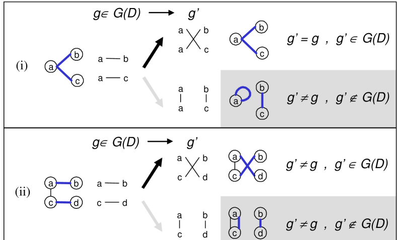
		Outcome from degree-preserving rewiring
		$g^{\prime}\in G(D)$		$g^{\prime}\not\in G(D)$
		simple		simple	not simple
		connected		not connected	not connected
Case/Motif	Count	$g^{\prime}=g$	$g^{\prime}\neq g$	$g^{\prime}\neq g$	$g^{\prime}\neq g$
(i)	$\frac{d^{2}}{2}-l$	1	0	0	1
(ii)	$s-d^{2}+l$	0	1	0	1
(iii)	$\frac{d^{2}}{2}-s+\frac{l^{2}-l}{2}$	0	1	1	0
Totals	$\frac{l^{2}-l}{2}$	$\frac{d^{2}}{2}-l$	$\frac{l^{2}+l}{2}-\frac{d^{2}}{2}$	$\frac{d^{2}}{2}-s+\frac{l^{2}-l}{2}$	$s-\frac{d^{2}}{2}$

Figure 8: (a) Three possible subgraph-based motifs in degree-preserving rewiring in acyclic graphs. Blue links represents links to be rewired. Rewiring operations that result in non-simple graphs (shaded) are assumed to revert to the original configuration. Thus defined, rewiring of motif (i) does not result in any new graphs, rewiring of motif (ii) results in one possible new graph, and rewiring of motif (iii) results in two possible new graphs. (b) The numbers of the three motifs and successively the number for each possible rewiring outcome. We distinguish between equal, not equal but connected and simple, not connected but simple, and not simple graphs that are similar to each graph with the given motif selected for rewiring. The total number of cases (column sum) is $(l^{2}-l)/2$, while the total number (row sum) of outcomes is twice that at $l^{2}-l$. Here, we use the abbreviated notation $d^{2}=\sum_{k}{d_{k}}^{2}$ and $s=s(g)$, with $l$ equal to the number of links in the graph.

4.4.1 Subgraph-Based Motifs

For any graph $g\in G(D)$, consider the set of local degree-preserving rewirings of distinct pairs of links. There are ${l\choose 2}=l(l-1)/2$ pairs of different links on which degree preserving rewiring can occur. Each pair of links defines its own network subgraph, and in the case where $g$ is an acyclic graph (i.e. a tree), these form three distinct types of subgraphs, as shown in Figure 8(a). Using the notation $d^{2}=\sum{d_{k}}^{2}$, $s=s(g)$ we can enumerate the number of these subgraphs as follows:

1. The two links share a common node. There are $\sum_{i=1}^{n}{d_{i}\choose 2}=\frac{1}{2}d^{2}-l$ possible ways that this can occur.

2. The links have two nodes that are connected by a third link. There are $\sum_{(i,j)\in\mathcal{E}}(d_{i}-1)(d_{j}-1)=s-d^{2}+l$ possible ways that this can occur.

3. The links have end points that do not share any direct connections. There are ${l\choose 2}-\sum_{i=1}^{n}{d_{i}\choose 2}-\sum_{(i,j)\in\mathcal{E}}(d_{i}-1)(d_{j}-1)=\frac{1}{2}d^{2}-s+\frac{1}{2}(l^{2}-2)$ possible ways that this can occur.

Collectively, these three basic subgraphs account for all possible ${l\choose 2}=l(l-1)/2$ pairs of different links. The subgraphs in cases (i) and (ii) are themselves trees, while the subgraph in case (iii) is not. We will refer to these three cases for subgraphs as “motifs”, in the spirit of [70], noting that our notion of subgraph-based motifs is motivated by the operation of random rewiring to be discussed below.

The simplest and most striking feature of the relationship between motifs and $s(g)$ for acyclic graphs is that we can derive formulas for the number of subgraph-based (local) motifs (and the outcomes of rewiring) entirely in terms of $d^{2}$, $s=s(g)$, and $l$. Thus, for example, we can see that graphs having higher $d^{2}$ (equivalently higher $CV$) values have fewer of the second motif. If we fix $D$, and thus $l$ and $d^{2}$, for all graphs of interest, then the only remaining dependence is on $s$, and graphs with higher $s(g)$-values contain fewer disconnected (case iii) motifs. This can be interpreted as a motif-level connection between $s(g)$ and self-similarity, in that graphs with higher $s(g)$ contain more motifs that are themselves trees, and thus more similar to the graph as a whole. Graphs having lower $s(g)$ have more motifs of type (iii) that are disconnected and thus dissimilar to the graph as a whole. Thus high-$s(g)$ graphs have this “motif self-similarity,” low-$s(g)$ graphs have “motif self-dissimilarity” and we can precisely define a measure of this kind of self-similarity and self-dissimilarity as follows.

Definition 2.

For a graph $g\in G(D)$, another measure of the extent to which $g$ is self-similar is the metric $ss(g)$ defined as the number of motifs (cases i-ii) that are themselves connected graphs. Accordingly, the measure of self-dissimilarity $sd(g)$ is then the number of motifs (case iii) that are disconnected.

For trees, $ss(g)=s-d^{2}/2$ and $sd(g)=-s+(l^{2}-l+d^{2})/2$, so this local motif self-similarity (self-dissimilarity) is essentially equivalent to high-$s(g)$ (resp. low-$s(g)$). As noted previously, network motifs have already been used as a way to study self-similarity and coarse graining [58, 59]. There, one defines a recursive procedure by which node connectivity patterns become represented as a single node (i.e. a different kind of motif), and it was shown that many important technological and biological networks were self-dissimilar, in the sense coarse-grained counterparts display very different motifs at each level of abstraction. Our notion of motif self-similarity is much simpler, but consistent, in that the Internet has extremely low $s(g)$ and thus minimally self-similar at the motif level. The next question is whether high $s(g)$ is connected with “self-similar” in the sense of being preserved under rewiring.

4.4.2 Degree-preserving Rewiring

We can also connect $s(g)$ in several ways with the effect that local rewiring has on the global structure of graphs in the set $G(D)$. Recall the above process by which two network links are selected at random for degree-preserving rewiring, and note that when applied to a graph $g\in G(D)$, there are four possible distinguishable outcomes:

1. $g^{\prime}=g$ with $g^{\prime}\in G(D)$: the new graph $g^{\prime}$ is equal to the original graph $g$ (and therefore also a simple, connected graph in $G(D)$);

2. $g^{\prime}\neq g$ with $g^{\prime}\in G(D)$: the new graph $g^{\prime}$ is not equal to $g$, but is still a simple, connected graph in the set $G(D)$ (note that this can include $g^{\prime}$ which are isomorphic to $g$);

3. $g^{\prime}=g$ with $g^{\prime}\not\in G(D)$: the new graph $g^{\prime}$ is still simple, but is not connected;

4. $g^{\prime}=g$ with $g^{\prime}\not\in G(D)$: the new graph $g^{\prime}$ is no longer simple (i.e. it either contains self-loops or parallel links).

There are two possible outcomes from the rewiring of any particular pair of links, as shown in Figure 8(a) and this yields a total of $2{l\choose 2}=l(l-1)$ possible outcomes of the rewiring process. In our discussion here, we ignore isomorphisms and assume that all non-equal graphs are different.

We are ultimately interested in retaining within our new definitions the notion that high $s(g)$ graphs are somehow preserved under rewiring provided this is sufficiently random and degrees are preserved. Scaling is of course trivially preserved by any degree-preserving rewiring, but high $s(g)$ value is not. Again, Figure 5 provides a clear example, since successive rewirings can take any of these graphs to any other. More interesting for high $s(g)$ graphs is the effect of random rewiring. Consider again the $\mbox{\em Perf}(g)$ vs. $s(g)$ plane from Figure 6. In addition to the four networks from Figure 5, we show the $\mbox{\em Perf}(g)$ and $s(g)$ values for other graphs in $G(D)$ obtained by degree-preserving rewiring from the initial four networks. This is done by selecting uniformly and randomly from the $l(l-1)$ different rewirings of the $l(l-1)/2$ different pairs of links, and restricting rewiring outcomes to elements of $G(D)$ by resetting all disconnected or nonsimple neighbors to equal. Points that match the color of one of the four networks are only one rewiring operation away, while points represented in gray are more than one rewiring operation away.

The connections of the results in Figure 8(b) to motif counts is more transparent however than to the consequences of successive rewiring. Nevertheless, we can use the results in Figure 8(b) to describe related ways in which low $s(g)$ graphs are “destroyed” by random rewiring. For any graph $g$, we can enumerate among all possible pairs of links on which degree preserving rewiring can take place and count all those that result in equal or non-equal graphs. In Figure 8, we consider the four cases for degree-preserving rewiring of acyclic graphs, and we count the number of ways each can occur. For motifs (i) and (ii), it is possible to check locally for outcomes that produce non-simple graphs and these cases correspond to the shaded outcomes in Figure 8(a). If we a priori exclude all such nonsimple rewirings, then there remain a total of $l(l-1)-s+d^{2}/2$ simple similar neighbors of a tree. We can define a measure of local rewiring self-dissimilarity for trees as follows.

Definition 3.

For a tree $g\in G(D)$, we measure the extent to which $g$ is self-dissimilar under local rewiring by the metric $rsd(g)$ defined as the number of simple similar neighbors that are disconnected graphs.

For trees, $rsd(g)=sd(g)=-s+(l^{2}-l+d^{2})/2$, so this local rewiring self-dissimilarity is identical to motif self-dissimilarity and directly related to low $s(g)$ values. This is because only motif (iii) results in simple but not connected similar neighbors.

4.5 A Coherent Non-Stochastic Picture

Here, we pause to reconsider the features/claims for SF graphs in the existing literature (Section 3.1) in light of our structural approach to graphs with scaling degree sequence $D$. In doing so, we make a simple observation: high-$s(g)$ graphs exhibit most of the features highlighted in the SF literature, but low-$s(g)$ graphs do not, and this provides insight into the diversity of graphs in the space $G(D)$. Perhaps more importantly, given a graph with scaling degree $D$ the $s(g)$ metric provides a “litmus test” as to whether or not the existing SF literature might be relevant to the network under study.

By definition, all graphs in $G(D)$ exhibit power laws in their node degrees provided that $D$ is scaling. However, preferential attachment mechanisms typically yield only high-$s(g)$ graphs—indeed the $s_{\max}$ construction uses what is essentially the “most preferential” type of attachment mechanism. Furthermore, while all graphs having scaling degree sequence $D$ have high-degree nodes or “hubs”, only for high-$s(g)$ graphs do such hubs tend to be critical for overall connectivity. While it is certainly possible to construct a graph with low $s(g)$ and having a central hub, this need not be the case, and our work to date suggests that most low-$s(g)$ graphs do not have the type of central hubs that create an “Achilles’ heel”. Additionally, we have illustrated that high-$s(g)$ graphs exhibit striking self-similarity properties, including that they are largely preserved under appropriately defined graph transformations of trimming, coarse graining and random pairwise degree-preserving rewiring. In the case of random rewiring, we offered numerical evidence and heuristic arguments in support of the conjecture that in general high-$s(g)$ graphs are the likely outcome of performing such rewiring operations, whereas low-$s(g)$ graphs are unlikely to occur as a result of this process.

Collectively, these results suggest that a definition of “scale-free graphs” that restricts graphs to having both scaling degree $D$ and high-$s(g)$ results in a coherent story. It recovers all of the structural results in the SF literature and provides a possible explanation why some graphs that exhibit power laws in their node degrees do not seem to satisfy other properties highlighted in the SF literature. This non-stochastic picture represents what is arguably a reasonable place to stop with a theory for “scale-free” graphs. However, from a graph theoretic perspective, there is considerable more work that could be done. For example, it may also be possible to expand the discussion of Section 4.4 to account more comprehensively for the way in which local motifs are transformed into one another and to relate our attempts more directly to the approach considered in [70]. Elaborating on the precise relationships and providing a possible interpretation of motifs as capturing a kind of local as well as global self-similarity property of an underlying graph remain open interesting problems. Additionally, we have also seen that the use of degree-preserving rewiring among connected graphs provides one view into the space $G(D)$. However, the geometry of this space is still complicated, and additional work is required to understand its remaining features. For example, our work to date suggests that for scaling $D$ it is impossible to construct a graph that has both high $\mbox{\em Perf}(g)$ and high $s(g)$, but this has not been proven. In addition, it will be useful to understand the way that degree-preserving rewiring causes one to “move” within the space $G(D)$ (see for example, [49, 46]).

It is important to emphasize that the purpose of the $s(g)$ metric is to provide insight into the structure of “scale free” graphs and not as a general metric for distinguishing among all possible graphs. Indeed, since the metric fails to distinguish among graphs having low $s(g)$, it provides little insight other than to say that there is tremendous diversity among such graphs. However, if a graph has high $s(g)$, then we believe that there exist strong properties that can be used to understand the structure (and possibly, the behavior) of such systems. In summary, if one wants to understand “scale-free graphs”, then we argue that $s(g)$ is an important metric and highly informative. However, for graphs with low $s(g)$ then this metric conveys limited information.

Despite the many appealing features of a theory that considers only non-stochastic properties, most of the SF literature has considered a framework that is inherently stochastic. Thus, we proceed next with a stochastic version of the story, one that connects more directly with the existing literature and common perspective on SF graphs.

5 A Probabilistic Approach

While the introduction and exploration of the $s$-metric fits naturally within standard studies of graph theoretic properties, it differs from the SF literature in that our structural approach does not depend on a probability model underlying the set of graphs of interest. The purpose of this section is to compare our approach with the more conventional probabilistic and ensemble-based views. For many application domains, including the Internet, there seems to be little motivation to assume networks are samples from an ensemble, and our treatment here will be brief while trying to cover this broad subject. Here again, we show that the $s(g)$ metric is potentially interesting and useful, as it has a direct relationship to notions of graph likelihood, graph degree correlation, and graph assortativity. This section also highlights the striking differences in the way that randomness is treated in physics-inspired approaches versus those shaped by mathematics and engineering.

The starting point for most probabilistic approaches to the study of graphs is through the definition of an appropriate statistical ensemble (see for example [40, Section 4.1]).

Definition 4.

A statistical ensemble of graphs is defined by

1. a set $G$ of graphs $g$, and

2. a rule that associates a real number (“probability”) $0\leq P(g)\leq 1$ with each graph $g\in G$ such that $\sum_{g\in G}P(g)=1$.

To describe an ensemble of graphs, one can either assign a specific weight to each graph or define some process (i.e., a stochastic generator) which results in a weight. For example, in one basic model of random graphs, the set $G$ consists of all graphs with vertex set $V=\{1,2,\ldots,n\}$ having $l$ edges, and each element in $G$ is assigned the same probability $1/{n\choose l}$. In an alternative random graph model, the set $G$ consists of all graphs with vertex set $V=\{1,2,\ldots,n\}$ in which the edges are chosen independently and with probability $0<p<1$. In this case, the probability $P(g)$ depends on the number of edges in $g$ and is given by $P(g)=p^{l}(1-p)^{n-l}$, where $l$ denotes the number of edges in $g\in G$.

The use of stochastic construction procedures to assign statistical weights has so dominated the study of graphs that the assumption of an underlying probability model often becomes implicit. For example, consider the four graph construction procedures listed in [40, p.22] that are claimed to form “the basis of network science,” and include (1) classical random graphs due to Erdös and Renyí [43]; (2) equilibrium random graphs with a given degree distribution such as the Generalized Random Graph (GRG) method [32]; (3) “small-world networks” due to Watts and Strogatz [109]; and (4) networks growing under the mechanism of preferential linking due to Barabási and Albert [15] and made precise in [24]. All of these construction mechanisms are inherently stochastic and provide a natural means for assigning, at least in principle, probabilities to each element in the corresponding space of realizable graphs. While deterministic (i.e., non-stochastic) construction procedures have been considered [20], their study has been restricted to the treatment of deterministic preferential attachment mechanisms that result in pseudofractal graph structures. Graphs resulting from other types of deterministic constructions are generally ignored in the context of statistical physics-inspired approaches since within the space of all feasible graphs, their likelihood of occurring is typically viewed as vanishingly small.

5.1 A Likelihood Interpretation of $s(g)$

Using the construction procedure associated with the general model of random graphs with a given expected degree sequence considered in [32] (also called the Generalized Random Graph (GRG) model for short) we show that the $s(g)$ metric allows for a more familiar ensemble-related interpretation as (relative) likelihood with which the graph $g$ is constructed according to the GRG method. To this end, the GRG model is concerned with generating graphs with given expected degree sequence $D=\{d_{1},\ldots d_{n}\}$ for vertices $1,\ldots,n$. The link between vertices $i$ and $j$ is chosen independently with probability $p_{ij}$, with $p_{ij}$ proportional to the product $d_{i}d_{j}$ (i.e. $p_{ij}=\rho d_{i}d_{j}$, where $\rho$ is a sufficiently small constant), and this defines a probability measure $P$ on the space of all simple graphs and thus induces a probability measure on $G(D)$ by conditioning on having degree $D$. The construction is fairly general and can recover the classic Erdös-Rényi random graphs [43] by taking the expected degree sequence to be $\{pn,pn,\ldots,pn\}$ for constant $p$. As a result of choosing each link $(i,j)\in\mathcal{E}$ with a probability that is proportional to $d_{i}d_{j}$ in the GRG model, different graphs are typically assigned different probabilities under $P$. This generation method is closely related to the Power Law Random Graph (PLRG) method [2], which also attempts to replicate a given (power law) degree sequence. The PLRG method involves forming a set $L$ of nodes containing as many distinct copies of a given vertex as the degree of that vertex, choosing a random matching of the elements of $L$, and applying a mapping of a given matching into an appropriate (multi)graph. It is believed that the PLRG and GRG models are “basically asymptotically equivalent, subject to bounding error estimates” [2]. Defining the likelihood of a graph $g\in G(D)$ as the logarithm of its probability under the measure $P$, we can show that the log likelihood (LLH) of a graph $g\in G(D)$, can be computed as

$$LLH(g)\approx\kappa+\rho\ s(g),$$ (10)

where $\kappa$ is a constant.

Note that the probability of any graph $g$ under $P$ is given by [77]

$$P(g) = \displaystyle{\prod_{(i,j)\in\mathcal{E}}p_{ij}\prod_{(i,j)\notin\mathcal{E}}(1-p_{ij})},$$

and using the fact that under the GRG model, we have $p_{ij}=\rho d_{i}d_{j}$, where $D=(d_{1},\ldots d_{n})$ is the given degree sequence, we get

$$P(g) = \rho^{l}\displaystyle{\prod_{i\in\mathcal{V}}d_{i}^{d_{i}}\prod_{(i,j)\notin\mathcal{E}}(1-\rho d_{i}d_{j})}$$

$$= \rho^{l}\displaystyle{\prod_{i\in\mathcal{V}}d_{i}^{d_{i}}\frac{\prod_{i,j\in\mathcal{V}}(1-\rho d_{i}d_{j})}{\prod_{(i,j)\in\mathcal{E}}(1-\rho d_{i}d_{j})}}.$$

Taking the log, we obtain

$$\log P(g) = l\log\rho+\displaystyle{\sum_{i\in\mathcal{V}}d_{i}\log d_{i}+\sum_{i,j\in\mathcal{V}}\log(1-\rho d_{i}d_{j})}$$

$$-{\sum_{(i,j)\in\mathcal{E}}\log(1-\rho d_{i}d_{j})}.$$

Defining

$$\kappa=l\log\rho+\displaystyle{\sum_{i\in\mathcal{V}}d_{i}\log d_{i}+\sum_{i,j\in\mathcal{V}}\log(1-\rho d_{i}d_{j})},$$

we observe that $\kappa$ is constant for fixed degree sequence $D$. Also recall that $\log(1+a)\approx a$ for $|a|<<1$. Thus, if $\rho$ is sufficiently small so that $p_{ij}=\rho d_{i}d_{j}<<1$, we get

$$LLH(g)=\log P(g)\approx\kappa+\sum_{(i,j)\in\mathcal{E}}\rho d_{i}d_{j}.$$

This shows that the graph likelihood $LLH(g)$ can be made proportional to $s(g)$ and thus we can interpret $s(g)/s_{\max}$ as relative likelihood of $g\in G(D)$, for the $s_{\max}$-graph has the highest likelihood of all graphs in $G(D)$. Choosing $\rho=1/\sum_{i\in\mathcal{V}}d_{i}=1/2l$ in the GRG formulation results in the expectation

$$E(d_{i})=\sum_{j=1}^{n}p_{ij}=\sum_{j=1}^{n}\rho d_{i}d_{j}=\rho d_{i}\sum_{j=1}^{n}d_{j}=d_{i}.$$

However, this $\rho$ may not have $p_{ij}=\rho d_{i}d_{j}<<1$ and can even make $p_{ij}>1$, particularly in cases when the degree sequence is scaling. Thus $\rho$ must often be chosen much smaller than $\rho=1/\sum_{i\in\mathcal{V}}d_{i}=1/2l$ to ensure that $p_{ij}<<1$ for all nodes $i,j$. In this case, the “typical” graph resulting from this construction with have degree sequence much less than $D$, however this sequence will be proportional to the desired degree sequence, $E(d_{i})\propto d_{i}$.

While this GRG construction yields a probability distribution on $G(D)$ by conditioning on having degree sequence $D$, this is not an efficient, practical method to generate members of $G(D)$, particularly when $D$ is scaling and it is necessary to choose $\rho<<1/2l$. The appeal of the GRG method is that it is easy to analyze and yields probabilities on $G(D)$ with clear interpretations. All elements of $G(D)$ will have nonzero probability with log likelihood proportional to $s(g)$. But even the $s_{max}$ graph may be extremely unlikely, and thus a naive Monte Carlo scheme using this construction would rarely yield any elements in $G(D)$. There are many conjectures in the SF literature that suggest that a wide variety of methods, including random degree-preserving rewiring, produce “essentially the same” ensembles. Thus it may be possible to generate probabilities on $G(D)$ that can both be analyzed theoretically and also provide a practical scheme to generate samples from the resulting ensemble. While we believe this is plausible, it’s rigorous resolution is well beyond the scope of this paper.

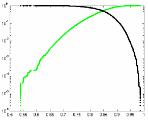
Figure 9: Results from Monte Carlo generation of preferential attachment graphs having 1000 nodes. For each trial, we compute the value $s(g)$ and then renormalize to $S(g)$ against the $s_{\max}$ graph having the same degree sequence. Both the CDF and CCDF are shown. In comparison, the HOTnet graph has $S(HOTnet)=0.3952$ and $S(HSFnet)=0.9791$.

5.2 Highly Likely Constructions

The interpretation of $s(g)$ as (relative) graph likelihood provides an explicit connection between this structural metric and the extensive literature on random graph models. Since the GRG method is a general means of generating random graphs, we can in principle generate random instances of “scale-free” graphs with a prescribed power law degree sequence, by using GRG as described above and then conditioning on that degree sequence. (And more efficient, practical schemes may also be possible.) In the resulting probability distribution on the space of graphs $G(D)$, high-$s(g)$ graphs with hub-like core structure are literally “highly likely” to arise at random, while low-$s(g)$ graphs with their high-degree nodes residing at the graphs’ peripheries are “highly unlikely” to result from such stochastic construction procedures.

While graphs resulting from stochastic preferential attachment construction may have a different underlying probability model than GRG-generated graphs, both result in simple graphs having approximate scaling relationships in their degree distributions. One can understand the manner in which high-$s(g)$ graphs are “highly likely” through the use of a simple Monte Carlo simulation experiment. Recall that the toy graphs in Figure 5 each contained 1000 nodes and that the graph in Figure 5(b) was “random” in the sense that it was obtained by successive arbitrary rewirings of HSFnet in Figure 5(a). An alternate approach to generating random graphs having a power law in their distribution of node degree is to use the type of preferential attachment mechanism first outlined in [15] and consider the structural features that are most “likely” among a large number of trials. Here, we generate 100,000 graphs each having 1000 nodes and measure the $s$-value of each. It is important to note that successive graphs resulting from preferential attachment will have different node degree sequences (one that is undoubtedly different from the degree sequence in Figure 5(e)), so a raw comparison of $s(g)$ is not appropriate. Instead, we introduce the normalized value $S(g)=s(g)/s_{\max}$ and use it to compare the structure of these graphs. Note that this means also generating the $s_{\max}$ graph associated with the particular degree sequence for the graph resulting from each trial. Fortunately, the construction procedure in Appendix A makes this straightforward, and so in this manner we obtain the normalized $S$-values for 100,000 graphs resulting from the same preferential attachment procedure. Plotting the CDF and CCDF of the $S$-values for these graphs in Figure 9, we observe a striking picture: all of the graphs resulting from preferential attachment had values of $S$ greater than 0.5, most of the graphs had values $0.6<S(g)<0.9$, and a significant number had values $S(g)>0.9$. In contrast, the graphs in Figure 5 had values: $S(HSFnet)=0.9791$, $S(Random)=0.8098$, $S(HOTnet)=0.3952$, and $S(PoorDesign)=0.4536$. Again, from the perspective of stochastic construction processes, low-$S$ values typical of HOT constructions are “very unlikely” while high-$S$ values are much more “likely” to occur at random.

With this additional insight into the $s$-values associated with different graphs, the relationship in the $\mbox{\em Perf}(g)$ vs. $s(g)$ plot of Figure 6 is clearer. Specifically, high-performance networks resulting from a careful design process are vanishingly rare from a conventional probabilistic graph point of view. In contrast, the likely outcome of random graph constructions (even carefully handcrafted ones) are networks that have extremely poor performance or lack the desired functionality (e.g., providing connectivity) altogether.

5.3 Degree Correlations

Given an appropriate statistical ensemble of graphs, the expectation of a random variable or random vector $X$ is defined as

$$\langle X\rangle=\sum_{g\in G}X(g)P(g).$$ (11)

For example, for $1\leq i\leq n$, let $D_{i}$ be the random variable denoting the degree of node $i$ for a graph $g\in G$ and let $D=\{D_{1},D_{2},\dots,D_{n}\}$ be the random vector representing the node degrees of $g$. Then the degree distribution is given by

$$P(k)\equiv P(\{g\in G:D_{i}(g)=k;i=1,2,\ldots,n\})$$

and can be written in terms of an expectation of a random variable, namely

$$P(k)=\frac{1}{n}\left\langle\sum_{i=1}^{n}\delta[D_{i}-k]\right\rangle$$

where

$$\delta[D_{i}(g)-k]=\left\{\begin{array}[]{ll}1&\mbox{if node }i\mbox{ of graph }g\mbox{ has degree }k\\ 0&\mbox{ otherwise.}\end{array}\right.$$

One previously studied topic has been the correlations between the degrees of connected nodes. To show that this notion has a direct relationship to the $s(g)$ metric, we follow [40, Section 4.6] and define the degree correlation between two adjacent vertices having respective degree $k$ and $k^{\prime}$ as follows.

Definition 5.

The degree correlation between two neighbors having degrees $k$ and $k^{\prime}$ is defined by

$$P(k,k^{\prime})=\frac{1}{n^{2}}\left\langle\sum_{i,j=1}^{n}\delta[d_{i}-k]a_{ij}\delta[d_{j}-k^{\prime}]\right\rangle$$ (12)

where the $a_{ij}$ are elements of the network node adjacency matrix such that

$$a_{ij}=\left\{\begin{array}[]{ll}1&\mbox{if nodes }i,j\mbox{ are connected}\\ 0&\mbox{ otherwise}\end{array}\right.$$

and where the random variables $\delta[D_{i}-k]$ are as above.

As an expectation of indicator-type random variables, $P(k,k^{\prime})$ can be interpreted as the probability that a randomly chosen link connects nodes of degrees $k$ and $k^{\prime}$, therefore $P(k,k^{\prime})$ is also called the “degree-degree distribution” for links. Observe that for a given graph $g$ having degree sequence $D$,

$$s(g) = \sum_{(i,j)\in\mathcal{E}}d_{i}d_{j}$$

$$= \sum_{(i,j)\in\mathcal{E}}\sum_{k\in D}k\delta[d_{i}-k]\sum_{k^{\prime}\in D}\delta[d_{j}-k^{\prime}]k^{\prime}$$

$$= \sum_{(i,j)\in\mathcal{E}}\sum_{k\in D}\sum_{k^{\prime}\in D}k\delta[d_{i}-k]\delta[d_{j}-k^{\prime}]k^{\prime}$$

$$= \frac{1}{2}\sum_{k,k^{\prime}\in D}kk^{\prime}\sum_{i,j=1}^{n}\delta[d_{i}-k]a_{ij}\delta[d_{j}-k^{\prime}]$$

Thus, there is an inherent relationship between the structural metric $s(g)$ and the degree-degree distribution, which we formalize as follows.

Proposition 6.

$$\langle s\rangle=\frac{n^{2}}{2}\sum_{k,k^{\prime}}kk^{\prime}P(k,k^{\prime}).$$ (13)

Proof of Proposition 6: For fixed degree sequence $D$,

$$\langle s\rangle = \left\langle\frac{1}{2}\sum_{k,k^{\prime}\in D}kk^{\prime}\sum_{i,j=1}^{n}\delta[d_{i}-k]a_{ij}\delta[d_{j}-k^{\prime}]\right\rangle$$

$$= \frac{1}{2}\sum_{k,k^{\prime}\in D}kk^{\prime}\left\langle\sum_{i,j=1}^{n}\delta[d_{i}-k]a_{ij}\delta[d_{j}-k^{\prime}]\right\rangle$$

$$= \frac{n^{2}}{2}\sum_{k,k^{\prime}\in D}kk^{\prime}P(k,k^{\prime}).$$

This result shows that for an ensemble of graphs having degree sequence $D$, the expectation of $s$ can be written purely in terms of the degree correlation. While other types of correlations have been considered (e.g., the correlations associated with clustering or loops in connectivity), degree correlations of the above type are the most obviously connected with the $s$-metric.

5.4 Assortativity/Disassortativity of Networks

Another ensemble-based notion of graph degree correlation that has been studied is the measure $r(g)$ of assortativity in networks as introduced by Newman [73], who describes assortative mixing ($r>0$) as “a preference for high-degree vertices to attach to other high-degree vertices” and disassortative mixing ($r<0$) as the converse, where “high-degree vertices attach to low-degree ones.” Since this is essentially what we have shown $s(g)$ measures, the connection between $s(g)$ and assortativity $r(g)$ should be and ultimately is very direct. As with all concepts in the SF literature, assortativity is developed in the context of an ensemble of graphs, but Newman provides a sample estimate of assortativity of any given graph $g$. Using our notation, Newman’s formula [73, Eq. 4] can be written as

$$r(g)=\frac{\left[\sum_{(i,j)\in\mathcal{E}}d_{i}d_{j}\right]-\left[\sum_{i\in\mathcal{V}}\frac{1}{2}d_{i}^{2}\right]^{2}/l}{\left[\sum_{i\in\mathcal{V}}\frac{1}{2}d_{i}^{3}\right]-\left[\sum_{i\in\mathcal{V}}\frac{1}{2}d_{i}^{2}\right]^{2}/l},$$ (14)

where $l$ is the number of links in the graph. Note that the first term of the numerator of $r(g)$ is precisely $s(g)$, and the other terms depend only on $D$ and not on the specific graph $g\in G(D)$. Thus $r(g)$ is linearly related to $s(g)$. However, when we compute $r(g)$ for the graphs in Figure 5 the values all are in the interval $[-0.4815,-0.4283]$. Thus all are roughly equally disassortative and $r(g)$ seems not to distinguish between what we have viewed as extremely different graphs. The assortativity interpretation appears to directly contradict both what appears obvious from inspection of the graphs, and the analysis based on $s(g)$. Recall that for $S(g)=s(g)/s_{\max}$ the graphs in Figure 5 had $S(HSFnet)=0.979$ and $S(HOTnet)=0.395$, with high-degree nodes in HSFnet attached to other high-degree nodes and in HOTnet attached to low-degree nodes.

The essential reason for this apparent conflict is that $-1\leq r(g)\leq 1$ and $0<S(g)\leq 1$ are normalized against a different “background set” of graphs. For $S(g)=s(g)/s_{\max}$ here, we have computed $s_{\max}$ constrained to simple, connected graphs, whereas $r(g)$ involves no such constraints. The $r=0$ graph with the same degree sequence as HSFnet and HOTnet would be non-simple—having, for example, the highest degree ($d_{1}$) node highly connected to itself (with multiple self-loops) and with multiple parallel connections to the other high-degree nodes (e.g. multiple links to the $d_{2}$ node). The corresponding $r=1$ graph would be both non-simple and disconnected—having the highest degree ($d_{1}$) node essentially connected only to itself. So HSFnet could be thought of as assortative when compared with graphs in $G(D)$, but dissassortative when compared with all graphs. To emphasize this distinction, the description of assortative mixing ($r>0$) could be augmented to “high-degree vertices attach to other high-degree vertices, including self-loops.” Since high variability, simple, connected graphs will all typically have $r(g)<0$, this measure is less useful than simply comparing raw $s(g)$ for this class of graphs. Thus conceptually, $r(g)$ and $s(g)$ have the same aim, but with different and largely incomparable normalizations, both of which are interesting.

We will now briefly sketch the technical details behind the normalization of $r(g)$. The first term of the denominator $\sum_{i\in\mathcal{V}}d_{i}^{3}/2l$ is equal to $s_{\max}$ for “unconstrained” graphs (i.e., those not restricted to be simple or even connected; see Appendix A for details), and the normalization term in the denominator can be understood accordingly as this $s_{\max}$. The term $\left(\sum_{i\in\mathcal{V}}d_{i}^{2}/2\right)^{2}/l$ can be interpreted as the “center” or zero assortativity case, again for unconstrained graphs. Thus, the perfectly assortative graph can be viewed as the $s_{\max}$ graph (within a particular background set $G$), and the assortativity of graphs is measured relative to the $s_{\max}$ graph, with appropriate centering.

Newman’s development of assortativity [73] is motivated by a definition that works both for an ensemble of graphs and as a sample-based metric for individual graphs. Accordingly, his definition depends on $Q(k,k^{\prime})$, the joint distribution of the remaining degrees of the two vertices at either end of a randomly selected link belonging to a graph in an ensemble. That is, consider a physical process by which a graph is selected from a statistical ensemble and then a link is arbitrarily chosen from that graph. The question of assortativity can then be understood in terms of some (properly normalized) statistical average between the degrees of the nodes at either end of the link. We defer the explicit connection between the ensemble-based and sample-based notions of assortativity and our structural metric $s(g)$ to Appendix B.

6 SF Graphs and the Internet Revisited

Given the definitions of $s(g)$, the various self-similarity and high likelihood features of high-$s(g)$ graphs, as well as the extreme diversity of the set of graphs $G(D)$ with scaling degree $D$, we look to incorporate this understanding into a theory of SF graphs that recovers both the spirit and existing results, while making rigorous the notion of what it means for a graph to be “scale-free”. To do so, we first trace the exact nature of previous misconceptions concerning the SF Internet, introduce an updated definition of a scale-free graph, clarify what statements in the SF literature can be recovered, and briefly outline the prospects for applying properly defined SF models in view of alternative theoretical frameworks such as HOT (Highly Optimized/Organized Tolerance/Tradeoffs). In this context, it is also important to understand the popular appeal that the SF approach has had. One reason is certainly its simplicity, and we will aim to preserve that as much as possible as we aim to replace largely heuristic and experimental results with ones more mathematical in nature. The other is that it relies heavily on methods from statistical physics, so much so that replacing them with techniques that are shaped by mathematics and engineering will require a fundamental change in the way complex systems such as the Internet are viewed and studied.

The logic of the existing SF theory and its central claims regarding the Internet consists of the following steps:

1. The claim that measurements of the Internet’s router-level topology can be reasonably modeled with a graph $g$ that has scaling degree sequence $D$.

2. The assertion, or definition, that a graph $g$ with scaling degree sequence $D$ is a scale-free graph.

3. The claim that scale-free graphs have a host of “emergent” features, most notably the presence of several highly connected nodes (i.e. “hubs”) that are critical to overall network connectivity and performance.

4. The conclusion that the Internet is therefore scale-free, and its “hubs,” through which most traffic must pass, are responsible for the “robust yet fragile” feature of failure tolerance and attack vulnerability.

In the following, we revisit the steps of this logic and illustrate that the conclusion in Step 4 is based on a series of misconceptions and errors, ranging in scope from taking highly ambiguous Internet measurements at face value to applying an inherently inconsistent SF theory to an engineered system like the Internet.

6.1 Scaling Degree Sequences and the Internet

The Internet remains one of the most popular and highly cited application areas where power laws in network connectivity have “emerged spontaneously”, and the notion that this increasingly important information infrastructure exhibits a signature of self-organizing complex systems has generated considerable motivation and enthusiasm for SF networks. However, as we will show here, this basic observation is highly questionable, and at worst is the simple result of errors emanating from the misinterpretation of available measurements and/or their naive and inappropriate statistical analysis of the type critiqued in Section 2.1.2

To appreciate the problems inherent in the available data, it is important to realize that Internet-related connectivity measurements are notorious for their ambiguities, inaccuracies, and incompleteness. This is due in part to the multi-layered nature of the Internet protocol stack (where each level defines its own connectivity), and it also results from the efforts of Internet Service Providers (ISPs) who intentionally obscure their network structure in order to preserve what they believe is a source of competitive advantage. Consider as an example the router-level connectivity of the Internet, which is intended to reflect (physical) one-hop distances between routers/switches. Although information about this type of connectivity is typically inferred from traceroute experiments which record successive IP-hops along paths between selected network host computers (see for example the Mercator [50], Skitter [34], and Rocketfuel [96] projects), there remain a number of challenges when trying to reverse-engineer a network’s physical infrastructure from traceroute-based measurements. The first challenge is that IP connectivity is an abstraction (at “Layer 3”) that sits on top of physical connectivity (at “Layer 2”), so traceroute is unable to record directly the network’s physical structure, and its measurements are highly ambiguous about the dependence between these two layers. Such ambiguity in Internet connectivity persists even at higher layers of the protocol stack, where connectivity becomes increasingly virtual, but for different reasons (see for example Section 6.4 below for a discussion of the Internet’s AS and Web graphs).

To illustrate how the somewhat subtle interactions among the different layers of the Internet protocol stack can give the (false) appearance of high connectivity at the IP-level, recall how at the physical layer the use of Ethernet technology near the network periphery or Asynchronous Transfer Mode (ATM) technology in the network core can give the appearance of high IP-connectivity since the physical topologies associated with these technologies may not be seen by IP-based traceroute. In such cases, machines that are connected to the same Ethernet or ATM network may have the illusion of direct connectivity from the perspective of IP, even though they are separated by an entire network (potentially spanning dozens of machines or hundreds of miles) at the physical level. In an entirely different fashion, the use of “Layer 2.5 technologies” such as Multiprotocol Label Switching (MPLS) tend to mask a network’s physical infrastructure and can give the illusion of one-hop connectivity at Layer 3. Note that in both cases, it is the explicit and intended design of these technologies to hide the physical network connectivity from IP. Another practical problem when interpreting traceroute data is to decide which IP addresses/interface cards (and corresponding DNS names) refer to the same router, a process known as alias resolution [95]. While one of the contributing factors to the high fidelity of the current state-of-the-art Rocketfuel maps is the use of an improved heuristic for performing alias resolution [96], further ambiguities remain, as pointed out for example in [107]. Yet another difficulty when dealing with traceroute-derived measurements has been considered in [64, 1] and concerns a potential bias whereby IP-level connectivity is inferred more easily and accurately the closer the routers are to the traceroute source(s). Such bias possibly results in incorrectly interpreting power law-type degree distributions when the true underlying connectivity structure is a regular graph (e.g., Erdös-Renyí [43]).

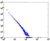
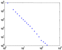
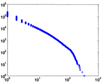
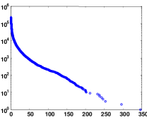
Figure 10: Traceroute-derived router-level connectivity data from the Mercator project [50]. (a) Doubly logarithmic size-frequency plot: Raw data. (b) Doubly logarithmic size-frequency plot: Binned data. (c) Doubly-logarithmic size-rank plot: Raw data with the 2 extreme nodes (with connectivity $>$ 1,000) removed. (d) Semi-logarithmic size-rank plot: Raw data with the 2 extreme nodes (with connectivity $>$ 1,000) removed.

Ongoing research continues to reveal new idiosyncrasies of traceroute-derived measurements and shows that their interpretation or analysis requires great care and diligent mining of other available data sources. Although the challenges associated with disambiguating the available measurements and identifying those contributions that are relevant for the Internet’s router-level topology can be daunting, using these measurements at face value and submitting them to commonly-used, black box-type statistical analyses—as is common in the complex systems literature—is ill-advised and bound to result in erroneous conclusions. To illustrate, Figure 10(a) shows the size-frequency plot for the raw traceroute-derived router-level connectivity data obtained by the Mercator project [50], with Figure 10(b) depicting a smoothed version of the plot in (a), obtained by applying a straightforward binning operation to the raw measurements, as is common practice in the physics literature. In fact, Figures 10(a)–(b) are commonly used in the SF literature (e.g., see [4]) as empirical evidence that the router-level topology of the Internet exhibits power-law degree distributions. However, in view of the above-mentioned ambiguities of traceroute-derived measurements, it is highly likely that the two extreme points with node degrees above 1,000 are really instances where the high IP-level connectivity is an illusion created by an underlying Layer 2 technology and says nothing about the actual connectivity at the physical level. When removing the two nodes in question and relying on the statistically more robust size-rank plots in Figures 10 (c) and (d), we notice that neither the doubly-logarithmic nor semi-logarithmic plots support the claim of a power law-type node degree distribution for the Internet’s router-level topology. In fact, Figures 10(c) and (d) strongly suggest that the actual router-level connectivity is more consistent with an exponentially-fast decaying node degree distribution, in stark contrast to what is typically claimed in the existing SF literature.

6.2 (Re)Defining “Scale-Free” Graphs

While it is unlikely that the Internet as a whole has scaling degree sequences, it would not be in principle technologically or economically infeasible to build a network which did. It would, however, be utterly infeasible to build a large network with high-degree SF hubs, or more generally one that had both high variability in node degree and large $s(g)$. Thus in making precise the definition of scale-free, there are essentially two possibilities. One is to define scale-free as simply having a scaling degree sequence, from which no other properties follow. The other is to define scale-free more narrowly in such a way that a rich set of properties are implied. Given the strong set of self-similarity properties of graphs $g$ having high $s(g)$, we propose the following alternate definition of what it means for a graph to be “scale-free”.

Definition 6.

For graphs $g\in G(D)$ where $D$ is scaling, we measure the extent to which the graph $g$ is scale-free by the metric $s(g)$.

This definition for “scale-free graphs” is restricted here to simple, connected graphs having scaling $D$, but $s(g)$ can obviously be computed for any graphs having any degree sequence, and thus defining $s(g)$ as a measure of “scale-free” might potentially be overly narrow. Nonetheless, in what follows, for degree sequences $D$ that are scaling, we will informally call graphs $g\in G(D)$ with low $s(g)$-values “scale-rich”, and those with high $s(g)$-values “scale-free.” Being structural in nature, this alternate definition has the additional benefit of not depending on a stochastic model underlying the set of graphs of interest. It does not rely on the statistical physics-inspired approach that focuses on random ensembles and their most likely elements and is inherent, for example, in the original Barabási-Albert construction procedure.

Our proposed definition for scale-free graphs requires that for a graph $g$ to be called scale-free, the degree sequence $D$ of $g$ must be scaling (or, more generally, highly variable) and self-similar in the sense that $s(g)$ must be large. Furthermore, $s(g)$ gives a quantitative measure of the extent to which a scaling degree graph is scale-free. In addition, this definition captures an explicit and obvious relationship between graphs that are “scale-free” and have a “hub-like core” of highly connected centrally-located nodes. More importantly, in view of Step 2 of the above-mentioned logic, the claim that scale-free networks have “SF hubs” is true with scale-free defined as scaling degree sequence and high $s(g)$, but false if scale-free were simply to mean scaling degree sequence, as is commonly assumed in the existing SF literature.

With a concise measure $s(g)$ and its connections with rich self-similarity/self-dissimilar properties and likelihood, we can look back and understand how both the appeal and failure of the SF literature is merely a symptom of much broader and deeper disconnects within complex networks research. First, while there are many possible equivalent definitions of scale-free, all nontrivial ones would seem to involve combining scaling degree with self-similarity or high likelihood and appear to be equivalent. Thus defined, models that generate scale-free graphs are easily constructed and are therefore not our main focus here. Indeed, because of the strong invariance properties of scaling distributions alone, it is easy to create limitless varieties of randomizing generative models that can “grow” graphs with scaling degree $D$. Preferential growth is perhaps the oldest of such models [117, 66, 94], so it is no surprise that it resurfaces prominently in the recent SF literature. No matter how scaling is generated however, the high likelihood and rewiring invariance of high-$s(g)$ graphs make it further easy—literally highly likely–to insure that these scaling graphs are also scale-free.

Thus secondly, the equivalence between “high $s$” and “highly likely” makes it possible to define scale-free as the likely or generic outcome of a great variety of random growth models. In fact, that “low $s$” or “scale-rich” graphs are vanishingly unlikely to occur at random explains why the SF literature has not only ignored their existence and missed their relevance but also conflated scale-free with scaling. Finally, since scaling and high $s$ are both so easily and robustly generated, requiring only few simple statistical properties, countless variations and embellishments of scale-free models have been proposed, with appealing but ultimately irrelevant details and discussions of emergence, self-organization, hierarchy, modularity, etc. However, their additional self-similarity properties, though still largely unexplored, have made the resulting scale-free networks intuitively appealing, particularly to those who continue to associate complexity with self-similarity.

The practical implication is that while our proposed definition of what it means for a graph to be “scale-free” recovers many claims in the existing SF literature, some aspects cannot be salvaged. As an alternate approach, we could accept a definition of scale-free that is equivalent to scaling, as is implicit in most of the SF literature. However, then the notion of “scale-free” is essentially trivial, and almost all claims in the existing literature about SF graphs are false, not just the ones specific to the Internet. We argue that a much better alternative is a definition of scale-free, as we propose, that implies the existence of “hubs” and other emergent properties, but is more restrictive than scaling. Our proposed alternative, that scale-free is a special case of scaling that further requires high $s(g)$, not only provides a quantitative measure about the extent to which a graph is scale-free, but also already offers abundant emergent properties, with the potential for a rigorous and rich theory.

In summary, notwithstanding the errors in the interpretation and analysis of available network measurement data, even if the Internet’s router-level graph were to exhibit a power law-type node degree distribution, we have shown here and in other papers (e.g., see [65, 110]) that the final conclusion in Step 4 is necessarily wrong for today’s Internet. No matter how scale-free is defined, the existing SF claims about the Internet’s router-level topology cannot be salvaged. Adopting our definitions, the router topology at least for some parts of the Internet could in principle have high variability and may even be roughly scaling , but it is certainly nowhere scale-free. It is in fact necessarily extremely “scale-rich” in a sense we have made rigorous and quantifiable, although the diversity of scale-rich graphs means that much more must be said to describe which scale-rich graphs are relevant to the Internet. A main lesson learned from this exercise has been that in the context of such complex and highly engineered systems as the Internet, it is largely impossible to understand any nontrivial network properties while ignoring all domain-specific details such as protocol stacks, technological or economic constraints, and user demand and heterogeneity, as is typical in SF treatments of complex networks.

6.3 Towards a Rigorous Theory of SF Graphs

Having proposed the quantity $s(g)$ as a structural measures of the extent to which a given graph is “scale-free”, we can now review the characteristics of scale-free graphs listed in Section 3 and use our results to clarify what is true if scale-free is taken to mean scaling degree sequence and large $s(g)$:

1. SF networks have scaling (power law) degree sequence (follows by definition).

2. SF networks are the likely outcome of various random growth processes (follows from the equivalence of $s(g)$ with a natural measure of graph likelihood).

3. SF networks have a hub-like core structure (follows directly from the definition of $s(g)$ and the betweeness properties of high-degree hubs).

4. SF networks are generic in the sense of being preserved by random degree-preserving rewiring (follows from the characterization of rewiring invariance of self-similarity).

5. SF networks are universal in the sense of not depending on domain-specific details (follows from the structural nature of $s(g)$).

6. SF networks are self-similar (is now partially clarified in that high $s(g)$ trees are preserved under both appropriately defined link trimming and coarse graining, as well as restriction to small motifs).

Many of these results are proven only for special cases and have only numerical evidence for general graphs, and thus can undoubtedly be improved upon by proving them in greater generality. However in most important ways the proposed definition is entirely consistent with the spirit of “scale-free” as it appears in the literature, as noted by its close relationship to previously defined notions of betweeness, assortativity, degree correlation, and so on. Since a high $s(g)$-value requires high-degree nodes to connect to other high-degree nodes, there is an explicit and obvious equivalence between graphs that are scale-free (i.e., have high $s(g)$-value) and have a “hub-like core” of highly connected nodes. Thus the statement “scale-free networks have hub-like cores”—while incorrect under the commonly-used original and vague definition (i.e., meaning scaling degree sequence)—is now true almost by definition and captures succinctly the confusion caused by some of the sensational claims that appeared in the scale-free literature. In particular, the consequences for network vulnerability in terms of the “Achilles’ heel” and a zero epidemic threshold follow immediately.

When normalized against a proper background set, our proposed $s(g)$-metric provides insight into the diversity of networks having the same degree sequence. On the one hand, graphs having $s(g)\approx s_{\max}$ are scale-free and self-similar in the sense that they appear to exhibit strong invariance properties across different scales, where appropriately defined coarse-graining operations (including link trimming) give rise to the different scales or levels of resolution. On the other hand, graphs having $s(g)<<s_{\max}$ are scale-rich and self-dissimilar; that is, they display different structure at different levels of resolution. While for scale-free graphs, degree-preserving random rewiring does not significantly alter their structural properties, even a modest amount of rewiring destroys the structure of scale-rich graphs. Thus, we suggest that a heuristic test as to whether or not a given graph is scale-free is to explore the impact of degree-preserving random rewiring. Recent work on the Internet [65] and metabolic networks [102] as well as on more general complex networks [112] demonstrates that many important large-scale complex systems are scale-rich and display significant self-dissimilarity, suggesting that their structure is far from scale-free and the opposite of self-similar.

6.4 SF Models and the Internet?

For the Internet, we have shown that no matter how scale-free is defined, the existing SF claims about the “robust, yet fragile” nature of these systems (particularly any claims of an “Achilles’ heel” type of vulnerability) are wrong no matter how scale-free is defined. By tracing through the reasoning behind these SF claims, we have identified the source of this error in the application of SF models to domains like engineering (or biology) where design, evolution, functionality, and constraints are all key ingredients that simply cannot be ignored. In particular, by assuming that scale-free is defined as scaling (or, more generally, highly variable) plus high $s(g)$, and further using $s(g)$ as a quantitative measure of how scale-free a graph is, the failure of SF models to correctly and usefully apply in an Internet-related context has been limited to errors due to ignoring domain-specific details, rather than to far more serious and general mathematical errors about the properties of SF graphs themselves. In fact, with our definition, there is the potential for a rich and interesting theory of SF graphs, looking for relevant and useful application domains.

One place where SF graphs may be appropriate and practically useful in the study of the Internet is at the higher levels of network abstraction, where interconnectivity is increasingly unconstrained by physical limitations. That is, while the lowest layers of the Internet protocol stack involving the physical infrastructure such as routers and fiber-optic cables have hard technological and economic constraints, each higher layer defines its own unique connectivity, and the corresponding network topologies become by design increasingly more virtual and unconstrained. For example, in contrast to routers and physical links, the connectivity structure defined by the documents (nodes) and hyperlinks (connections) in the World Wide Web (WWW) is designed to be essentially completely unconstrained. While we have seen that it is utterly implausible that SF models can capture the essential features of the router-level connectivity in today’s Internet, it seems conceivable that they could represent virtual graphs associated with the Internet such as, hypothetically, the WWW or other types of overlay networks.

However, even in the case of more virtual-type graphs associated with the Internet, a cautionary note about the applicability of SF models is needed. For example, consider the Internet at the level of autonomous systems, where an autonomous system (AS) is a subnetwork or domain that is under its own administrative control. In an AS graph representation of the Internet, each node corresponds to an AS and a link between two nodes indicates the presence of a “peering relationship” between the two ASes—a mutual willingness to carry or exchange traffic. Thus, a single “node” in an AS graph (e.g., AS 1239 is the Sprintlink network) represents potentially hundreds or thousands of routers as well as their interconnections. Although most large ASes have several connections (peering points) to other ASes, the use of this representation means that one is collapsing possibly hundreds of different physical (i.e., router-level) connections into a single logical link between two ASes. In this sense, the AS graph is expressively not a representation of any physical aspect of the Internet, but defines a virtual graph representing business (i.e., peering) relationships among network providers (i.e., ASes). Significant attention has been directed toward discovering the structural aspects of AS connectivity as represented by AS graphs and inferred from BGP-based measurements (where the Border Gateway Protocol or BGP is the de facto standard inter-AS routing protocol deployed in today’s Internet [100, 88]) and speculating on what these features imply about the large-scale properties of the Internet. However, the networking significance of these AS graphs is very limited since AS connectivity alone says little about how the actual traffic traverses the different ASes. For this purpose, the relevant information is encoded in the link type (i.e., peering agreement such as peer-to-peer or provider-customer relationship) and in the types of routing policies used by the individual ASes to enforce agreed-upon business arrangements between two or more parties.

In addition, due to the infeasibility of measuring AS connectivity directly, the measurements that form the basis for inferring AS-level maps consist of BGP routing table snapshots collected, for example, by the University of Oregon Route Views Project [88]. To illustrate the degree of ambiguity in the inferred AS connectivity data, note for example that due to the way BGP routing works, snapshots of BGP routing tables taken at a few vantage points on the Internet over time are unlikely to uncover and capture all existing connections between ASs. Indeed, [30] suggests that AS graphs inferred from the Route Views data typically miss between 20-50% or even more of the existing AS connections. This is an example of the general problem of vantage point mentioned in [81], whereby the location(s) of exactly where the measurements are performed can significantly skew the interpretation of the measurements, often in quite non-intuitive ways. Other problems that are of concern in this context have to do with ambiguities that can arise when inferring the type of peering relationships between two ASes or, more importantly, with the dynamic nature of AS-level connectivity, whereby new ASes can join and existing ASes can leave, merge, or split at any time.

This dynamic aspect is even more relevant in the context of the Web graph, another virtual graph associated with the Internet that is expressively not a representation of any physical aspect of the Internet structure but where nodes and links represent pages and hyperlinks of the WWW, respectively. Thus in addition to the deficiencies mentioned in the context of router-level Internet measurements, the topologies that are more virtual and “overlay” the Internet’s physical topology exhibit an aspect of dynamic changes that is largely absent on the physical level. This questions the appropriateness and relevance of a careful analysis or modeling of commonly considered static counterparts of these virtual topologies that are typically obtained by accumulating the connectivity information contained in a number of different snapshots taken over some time period into a single graph.

When combined, the virtual nature of AS or Web graphs and their lack of critical networking-specific information make them awkward objects for studying the “robust yet fragile” nature of the Internet in the spirit of the “Achilles’ heel” argument [6] or largely inappropriate structures for investigating the spread of viruses on the Internet as in [21]. For example, what does it mean to “attack and disable” a node such as Sprintlink (AS 1239) in a representation of business relationships between network providers? Physical attacks at this level are largely meaningless. On the other hand, the economic and regulatory environment for ISPs remains treacherous, so questions about the robustness (or lack thereof) of the Internet at the AS-level to this type of disruption seem appropriate. And even if one could make sense of physically “attacking and disabling” nodes or links in the AS graph, any rigorous investigation of its “robust yet fragile” nature would have to at least account for the key mechanisms by which BGP detects and reacts to connectivity disruptions at the AS level. In fact, as in the case of the Internet’s router-level connectivity, claims of scale-free structure exhibited by inferred AS graphs fail to capture the most essential “robust yet fragile” features of the Internet because they ignore any significant networking-specific information encoded in these graphs beyond connectivity. Again, the actual fragilities are not to physical attacks on AS nodes but to AS-related components “failing on,” particularly via BGP-related software or hardware components working improperly or being misconfigured, or via malicious exploitation or hijacking of BGP itself.

6.5 The Contrasting Role of Randomness

To put our SF findings in a broader context, we briefly review an alternate approach to the use of randomness for understanding system complexity that implicitly underpins our approach in a way similar to how statistical physics underpins the SF literature. Specifically, the notions of Highly Optimized Tolerance (HOT) [28] or Heuristically Organized Tradeoffs [44] has been recently introduced as a conceptual framework for capturing the highly organized, optimized, and “robust yet fragile” structure of complex highly evolved systems [29]. Introduced in the spirit of canonical models from statistical physics—such as percolation lattices, cellular automata, and spin glasses—HOT is an attempt to use simple models that capture some essence of the role of design or evolution in creating highly structured configurations, power laws, self-dissimilarity, scale-richness, etc. The emphasis in the HOT view is on “organized complexity”, which contrasts sharply with the view of “emergent complexity” that is preferred within physics and the SF community. The HOT perspective is motivated by biology and technology, and HOT models typically involve optimizing functional objectives of the system as a whole, subject to constraints on their components, usually with an explicit source of uncertainty against which solutions must be tolerant, or robust. The explicit focus on function, constraints, optimization, and organization sharply distinguish HOT from SF approaches. Both consider robustness and fragility but reach opposite and incompatible conclusions.

A toy model of the HOT approach to modeling the router-level Internet was already discussed earlier. The underlying idea is that consideration of the economic and technological factors constraining design by Internet Service Providers (ISPs) gives strong incentives to minimize the number and length of deployed links by aggregating and multiplexing traffic at all levels of the network hierarchy, from the periphery to the core. In order to efficiently provide high throughput to users, router technology and link costs thus necessitate that by and large link capacities increase and router degrees decrease from the network’s periphery to its more aggregated core. Thus, the toy model HOTnet in Figure 5(d), like the real router-level Internet, has a mesh of uniformly high-speed low connectivity routers in its core, with greater variability in connectivity at its periphery. While a more detailed discussion of these factors and additional examples is available from [65, 41], the result is that this work has explained where within the Internet’s router-level topology the high degree nodes might be and why they might be there, as well as where they can’t possibly be.

The HOT network that results is not just different than the SF network but completely opposite, and this can be seen not only in terms relevant to the Internet application domain, such as the performance measure (7), robustness to router and link losses, and the link costs, but in the criteria considered within the SF literature itself. Specifically, SF models are generated directly from ensembles and random processes, and have generic microscopic features that are preserved under random rewiring. HOT models have highly structured, rare configurations which are destroyed by random rewiring, unless that is made a specific design objective. SF models are universal in ignoring domain details, whereas HOT is only universal in the sense that it formulates everything in terms of robust, constrained optimization, but with highly domain-specific performance objectives and constraints.

One theme of the HOT framework has been that engineering design or biological evolution easily generates scaling in a variety of toy models once functional performance, component constraints, and robustness tradeoffs are considered. Both SF and HOT models of the Internet yield power laws, but once again in opposite ways and with opposite consequences. HOT emphasizes the importance of high variability over power laws per se, and provides a much deeper connection between variability or scaling exponents and domain-specific constraints and features. For example, the HOT Internet model considered here shows that if high variability occurs in router degree it can be explained by high variability in end user bandwidth together with constraints on router technology and link costs. Thus HOT provides a predictive model regarding how different external demands or future evolution of technology could change network statistics. The SF models are intrinsically incapable of providing such predictive capability in any application domain. The resulting striking differences between these two modeling approaches and their predictions are merely symptomatic of a much broader gap between the popular physics perspective on complex networks versus that of mathematics and engineering, created by a profoundly different perspective on the nature and causes of high variability in real world data. For example, essentially the same kind of contrast holds for HOT and SOC models [29], where SOC is yet another theoretical framework with specious claims about the Internet [97, 11].

In contrast to the SF approach, the HOT models described above as well as their constraints and performance measures do not require any assumptions, implicit or explicit, that they were drawn directly from some random ensemble. Tradeoffs in the real Internet and biology can be explained without insisting on any underlying random models. Sources of randomness are incorporated naturally where uncertainty needs to be managed or accounted for, say for the case of the router-level Internet, in a stochastic model of user bandwidth demands and geographic locations of users, routers, and links, followed by a heuristic or optimal design. This can produce either an ensemble of network designs, or a single robust design, depending on the design objective, but all results remain highly constrained and are characterized by low $s(g)$ and high $\mbox{\em Perf}(g)$. This is typical in engineering theories, where random models are common but not required, and where uncertainty can be modeled with random ensembles or worst-case over sets. In all cases, uncertainty models are mixed with additional hard constraints, say on component technology.

In the SF literature, on the other hand, random graph models and statistical physics-inspired approaches to networks are so deep-rooted that an underlying ensemble is taken for granted. Indeed, in the SF literature the phrase “not random” typically does not refer to a deterministic process but means random processes having some non-uniform or high variability distribution, such as scaling. Furthermore, random processes are used to directly generate SF network graphs rather than model uncertainty in the environment, leading in this case to high $s(g)$ and low $\mbox{\em Perf}(g)$ graphs. This particular view of randomness also blurs the important distinction between what is unlikely and what is impossible. That is, what is unlikely to occur in a random ensemble (e.g. a low $s(g)$ graph) is treated as impossible, while what is truly impossible (e.g. an Internet with SF hubs) from an engineering perspective is viewed as likely from an ensemble point of view. Similarly, the relation between high variability, scaling, and scale-free is murky in the SF literature. These distinctions may all be irrelevant for some scientific questions, but they are crucial in the study of engineering and biology and also essential for mathematical rigor.

7 A HOT vs. SF View
of Biological Networks

This section describes how a roughly parallel SF vs HOT story exists in metabolic networks, which is another application area that has been very popular in the SF and broader “complex networks” literature [19] and is also discussed in more detain in [48]. Recent progress has clarified many features of the global architecture of biological metabolic networks [36]. We argue here that they have highly organized and optimized tolerances and tradeoffs for functional requirements of flexibility, efficiency, robustness, and evolvability, with constraints on conservation of energy, redox, and many small moieties. These are all canonical examples of HOT features, and are largely ignored in the SF literature. One consequence of this HOT architecture is a highly structured modularity that is self-dissimilar and scale-rich, as in the Internet example. All aspects of metabolism have extremes in homogeneity and heterogeneity, and low and high variability, including power laws, in both metabolite and reaction degree distributions. We will briefly review the results in [102] which illustrate these features using the well-understood stoichiometry of metabolic networks in bacteria.

One difficulty in comparing SF and HOT approaches is that there is no sense in which ordinary (not bipartite) graphs can be used to meaningfully describe metabolism, as we will make clear below. Thus one would need to generalize our definition of scale-free to bipartite graphs just to precisely define what it would mean for metabolism to be scale-free. While this is an interesting direction not pursued here, the SF literature has many fewer claims about bipartite graphs, and they are typically studied by projecting them down onto one set of vertices. What is clear is that no definition can possibly salvage the claim that metabolism is scale-free, and we will pursue this aspect in a more general way. The rewiring-preserved features of scale-free networks would certainly be a central feature of any claim that metabolism is scale-free. This is also a feature of the two other most prominent “emergent complexity” models of biological networks, edge-of-chaos (EOC) and self-organized criticality (SOC). While EOC adds boolean logic and SOC adds cellular automata to the graphs of network connectivity, both are by definition unchanged by random degree-preserving rewiring. In fact, they are preserved under much less restrictive rewiring processes. Thus while there are currently no SF, EOC, or SOC models that apply directly to metabolic networks, we can clearly eliminate them a priori as candidate theories by showing that all important biochemical features of real metabolic networks are completely disrupted by rewirings that are far more restrictive than what is by definition allowable in SF, EOC, or SOC models.

7.1 Graph Representation

Cellular metabolism is described by a series of chemical reactions that convert nutrients to essential components and energy within the cell, subject to conservation constraints of atoms, energy and small moieties. The simplest model of metabolic networks is a stoichiometry matrix, or s-matrix for short, with rows of metabolites and columns of reactions. For example, for the set of chemical reactions

$$\left\{\begin{array}[]{*{20}c}{S_{1}+{\rm NADH}\to S_{2}+{\rm NAD}},\\ {S_{2}+{\rm ATP}\leftrightarrow S_{3}+{\rm ADP}},\\ {S_{4}+{\rm ATP}\to S_{5}+{\rm ADP}},\\ \end{array}\right.$$ (15)

we can write the associated stoichiometry matrix, or s-matrix, as

$$\begin{array}[]{*{20}c}{}\hfil&{{\rm{Reactions}}}\\ {}\hfil&{\begin{array}[]{*{20}c}{R_{1}}&{R_{2}}&{R_{3}}\\ \end{array}}\\ {\begin{array}[]{*{20}c}{{\rm{Substrates\hfill}}}&{\left\{{\begin{array}[]{*{20}c}{S_{1}}\\ {S_{2}}\\ {S_{3}}\\ {S_{4}}\\ {S_{5}}\\ \end{array}}\right.\hfill}\\ {{\rm{Carriers\hfill}}}&{\left\{{\begin{array}[]{*{20}c}{\rm ATP}\\ {\rm ADP}\\ {\rm NADH}\\ {\rm NAD}\\ \end{array}}\right.\hfill}\\ \end{array}}&{\left[{\begin{array}[]{*{20}c}{-1}&0&0\\ 1&{-1}&0\\ 0&1&0\\ 0&0&{-1}\\ 0&0&1\\ 0&{-1}&{-1}\\ 0&1&1\\ {-1}&0&0\\ 1&0&0\\ \end{array}}\right]}\\ \end{array}$$ (16)

with the metabolites in rows and reactions in columns. This is the simplest model of metabolism and is defined unambiguously except for permutations of rows and columns, and thus makes an attractive basis for contrasting different approaches to complex networks [19, 40, 55, 84].

Reactions in the entire network are generally grouped into standard functional modules, such as catabolism, amino acid biosynthesis, nucleotide biosynthesis, lipid biosynthesis and vitamin biosynthesis. Metabolites are categorized largely into carrier and non-carrier substrates as in rows of (16). Carrier metabolites correspond to conserved quantities, are activated in catabolism, and act as carriers to transfer energy by phosphate groups, hydrogen/redox, amino groups, acetyl groups, and one carbon units throughout all modules. As a result, they appear in many reactions. Non-carrier substrates are categorized further into precursor and other (than precursor and carrier) metabolites. The  12 precursor metabolites are outputs of catabolism and are the starting points for biosynthesis, and together with carriers make up the “knot” of the “bow-tie” structure [36] of the metabolism. The other metabolites occur primarily in separate reaction modules.

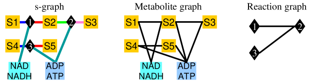
Figure 11: Graph representations of enzymatically catalyzed reactions from equation (15) having the s-matrix in equation (16). An s-graph consists of reaction nodes (black diamonds), non-carrier metabolite nodes (orange squares), and carrier metabolite nodes (light blue squares). Red and blue edges correspond to positive and negative elements in the stoichiometry matrix, respectively, for irreversible reactions, and pink and green ones correspond to positive and negative elements, respectively, for reversible reactions. All the information in the s-matrix appears schematically in the s-graph. Carriers which always occur in pairs (ATP/ADP, NAD/NADH etc.) are grouped for simplification. Corresponding metabolite graphs containing only metabolite nodes and reaction graph containing only reaction nodes lose important biochemical information. Note that all metabolites and reactions are “close” in the metabolite and reaction graphs, simply because they share common carriers, but could be arbitrarily far apart in any real biochemical sense. For example, reactions 2 and 3 could be in amino acid and lipid biosynthesis, respectively, and thus would be far apart biochemically and in the s-graph.

The information conveyed in the s-matrix can be represented in a color-coded bipartite graph, called an s-graph [102] (Figure 11), where both reactions and metabolites are represented as distinct nodes and membership relationships of metabolites to reactions are represented by links. With the color-coding of links indicating the reversibility of reactions and the sign of elements in the s-matrix, all the biochemical information contained in the s-matrix is accurately reflected in the s-graph. One of the most important features of s-graphs of this type is the differentiation between carrier (e.g. ATP) and non-carrier metabolites that help to clarify biochemically meaningful pathways. An s-graph for a part of amino acid biosynthesis module of H. Pylori is shown in Figure 12. The objective of each functional module is to make output metabolites from input metabolites through successive reactions. The enzymes of core metabolism are highly efficient and specialized, and thus necessarily have few metabolites and involve simple reactions [102]. As a result, long pathways are required biochemically to build complex building blocks from simpler building blocks within a function module. Long pathways are evident in the s-graph in Figure 12.

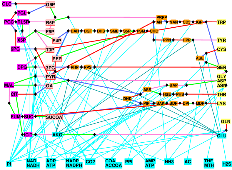
Figure 12: An s-graph for part of the catabolism and amino acid biosynthesis module of H.Pylori. The conventions are the same as those in Figure 11. This illustrates that long biosynthetic pathways build complex building blocks (in yellow on the right) from precursors (in orange on the left) in a series of simple reactions (in the middle), using shared common carriers (at the bottom). Each biosynthetic module has a qualitatively similar structure.

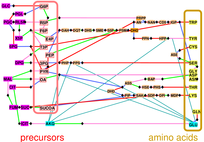
Figure 13: The s-graph in Figure 12 with carriers deleted to highlight the long assembly pathways. Note that there are no high degree “hub” nodes responsible for the global connectivity of this reduced s-graph. AKG and GLU are carriers for amino groups, and this role has been left in.

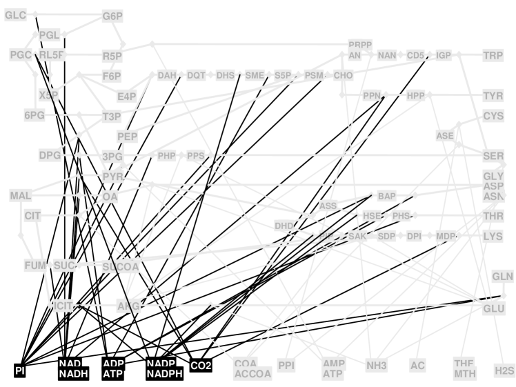
Figure 14: High connectivity metabolites in the s-graph in Figure 12 are these carriers which are not directly involved in the pathways. Because carriers are shared throughout metabolism, they are entirely responsible for the presence of high variability in metabolite degree, and thus the presence of scaling in metabolism.

Simpler representations of the information in the s-graph are possible, but only at a cost of losing significant biochemical information. A metabolite graph in which nodes represent only metabolites and are “connected” when they are involved in the same reaction, or a reaction graph in which nodes represent only reactions and are “connected” when they contain common metabolites (both shown in Figure 11) destroys much of the rich structure and biochemical meaning when compared to the s-graph. (The metabolite graphs are sometimes further reduced by deleting carriers.) Nonetheless, many recent studies have emphasized the connectivity features of these graphs, and reports of power laws in some of the degree distribution have been cited as claims that (1) metabolic networks are also scale-free [19] and (2) the presence of highly connected hubs and self-similar modularity capture much of the essential details about ”robust yet fragile” feature of metabolism [84]. Here, highly connected nodes are carriers, which are shared throughout metabolism.

We will first clarify why working with any of these simple graphs of metabolism, rather than the full s-graph, destroys their biochemical meaning and leads to a variety of errors. Consider again the simple example of Equation (15) and its corresponding s-matrix (16). Here, assume that reactions $R_{1}$ and $R_{2}$ are part of the pathways of a functional module, say amino acid biosynthesis, and reaction $R_{3}$ is in another module, say lipid biosynthesis. Then the metabolite and reaction graphs both show that substrates $S_{3}$ and $S_{4}$, as well as reactions $R_{2}$ and $R_{3}$ are “close” simply because they share ATP/ADP. However, since they are in different functional modules, they are not close in any biologically meaningful sense. (Similarly, two functionally different and geographically distant appliances are not “close” in any meaningful sense simply because both happen to be connected to the US power grid.) Attempts to characterize network diameter are meaningless in such simplified metabolite graphs because they fail to extract biochemically meaningful pathways. Additional work using structural information of metabolites with carbon atomic traces [10] has clarified that the average path lengths between all pairs of metabolites in E. coli is much longer than has been suggested by approaches that consider only simplistic connectivity in metabolite graphs. “Achilles’ heel” statements [6] for metabolic networks are particularly misleading. Eliminating, say, ATP from a cell is indeed lethal but the explanation for this must involve its biochemical role, not its graph connectivity. Indeed, the “Achilles’ heel” arguments suggest that removal of the highly connected carrier “hub” nodes would fragment the graph, but Figure 13 shows that removing the carriers from biologically meaningful s-graph in Figure 12 still yields a connected network with long pathways between the remaining metabolites. If anything, this reduced representation highlights many of the more important structural feature of metabolism, and most visualizations of large metabolic networks use a similar reduction. Attempts to “fix” this problem by a priori eliminating the carriers from metabolite graphs results in graphs with low variability in node degree and thus are not even scaling, let alone scale-free. Thus the failure of the SF graph methods to explain in any way the features of metabolism is even more serious than for the Internet.

7.2 Scale-rich metabolic networks

Recent work [102] has clearly shown the origin of high variability in metabolic networks by consideration of both their constraints and functional requirements, together with biochemically meaningful modular decomposition of metabolites and reactions shown above. Since maintaining a large genome and making a variety of enzymes is costly, the total number of reactions in metabolism must be kept relatively small while providing robustness of the cell against sudden changes, often due to environmental fluctuations, in either required amount of products or in available nutrients. In real metabolic networks, scaling only arises in the degree distribution of total metabolites. The reaction node degree distribution shows low variability because of the specialized enzymes which allow only a few metabolites in each reaction. High variability in metabolite node degrees is a result of the mixture of a few high degree shared carriers with many other low degree metabolites unique to each function module, with the precursors providing intermediate degrees. Thus, the entire network is extremely scale-rich, in the sense that it consists of widely different scales and is thus fundamentally self-dissimilar.

Scale-richness of metabolic networks has been evaluated quantitatively in [103] by degree-preserving rewiring of real stoichiometry matrices, which severely alters their structural properties. Preserving only the metabolite degrees gives much higher variability in reaction node degree distribution than is possible using simple enzymes, and rewiring also destroys conservation of redox and moieties. The same kind of degree-preserving rewiring on a simple HOT model [104], proposed with the essential feature of metabolism, such as simple reactions, shared carriers, and long pathways, has reinforced these conclusions but in a more analytical framework [103]. Even (biologically meaningless) metabolite graphs have a low $S(g)$ value, and are thus scale-rich, not scale-free. The simple reactions of metabolism require that the high-degree carriers are more highly connected to low-degree metabolites than to each other, as is shown in the metabolite graph in Figure 11, yielding a relatively low $s(g)$ value. Figure 15 shows the $s(g)$ values for the H. Pylori metabolite graph compared with those for graphs obtained by random degree-preserving rewiring of that graph.

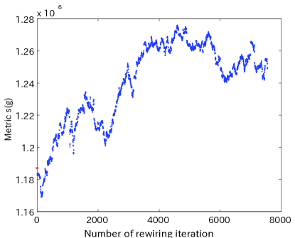
Figure 15: Metric $s(g)$ for real metabolite graph for H. Pylori ($\ast$) and those for graphs obtained by degree-preserving random rewiring.

Even the most restrictive possible rewiring destroys the structure of metabolism, showing that no SF, SOC, or EOC models are possible, even in principle. Suppose we freeze the role of carriers in each reaction, and then allow only rewiring of the remaining metabolites. This would be equivalent to Figure 13 with the carrier for amino group roles of AKG and GLU also frozen. What then remains is nearly a tree, and thus the rewiring counts from Figure 8 are approximately correct. Note that half of all rewirings disconnect a tree, and monte carlo numerical experiments of successive rewirings produces a jumble of futile cycles and short, dead end pathways[103]. The long assembly lines of real metabolism are extremely rare configurations and highly scale-rich, and are vanishingly unlikely to arise by any random ensemble model such as in SF, SOC, or EOC theories.

Real metabolic networks are scale-rich in every conceivable interpretation, and cannot be scale-free in any sense consistent with the either the definitions in this paper or with the spirit of the SF literature. In contrast to any approach that treats metabolic networks as generic, a biological perspective requires that the organization of metabolic networks be discussed with emphasis on the functional requirements of conversion of nutrients to products with flexibility, efficiency, robustness, and evolvability under the constraints on enzyme costs and conservation of energy, redox, and many small moieties [35, 99]. This structure is a natural consequence of a highly optimized and structured tradeoff (HOT) “bow-tie” structure, which facilitates great robustness and efficiency but is also a source of vulnerability, but primarily to hijacking and fail-on of components [36, 104, 99]. A power law in metabolite degree is simply the natural null hypothesis with any structure that exhibits high variability by shared carriers, and thus is by itself not suggestive of any further particular mechanism.

Another prominent example of biologic networks claimed to be SF [54, 116] is protein-protein interaction (PPI) networks. This claim has lead to conclude that identifying high-degree ”hub” proteins reveals important features of PPI networks. However, recent analysis [105] evaluating the claims that PPI node degree sequences follow a power law, a necessary condition for networks to be SF, shows that the node degree sequences of some published refined PPI networks do not have power laws when analyzed correctly using the cumulative plots as discussed in Section 2.1. Thus these PPI networks are not SF networks. It is in principle possible that the data studied in [105] is misleading because of the small size of the network and potential experimental errors, and that real PPI networks might have some features attributed to SF networks. At this time we only can draw conclusions about (noisy) subgraphs of the true PPI network since the data sets are incomplete and presumably contain errors. If it is true that appropriately sampled subraphs of a SF graph is SF as was claimed in [116], they possess a power law node degree sequence. That these subgraphs exhibit exponential node degree sequences suggests that the entire network is not SF. Since essentially all the claims that biological networks are SF are based on ambiguous frequency-degree analysis, this analysis must be redone to determine the correct form of the degree sequences. Analysis in [105] has provided clear examples that ambiguous plots of frequency-degree could lead to erroneous conclusion on the existence and parametrization of power law relationships.

As we have shown above, cell metabolism plausibly can have power laws for some data sets, but have none of the other features attributed to SF networks. Metabolic networks have been shown to be scale-rich (SR), in the sense that they are far from self-similar [102] despite some power laws in certain node degree sequence. Their power law node degree sequence is a result of the mixture of exponential distributions in each functional module, with carriers playing a crucial role. In principle, PPI networks could have this SR structure as well, since their subnetworks have exponential degree sequence, and perhaps power laws could emerge at higher levels of organization. This will be revealed only when a more complete network is elucidated. Still, the most important point is not whether the node degree sequence follows a power law, but whether the variability of the node degree sequences is high or low, and the biological protocols that necessitate this high or low variability. These issues will be explored in future publications.

8 Conclusions

The set $G(D)$ of graphs $g$ with fixed scaling degree $D$ is extremely diverse. However, most graphs in $G(D)$ are, using our definition, scale-free and have high $s$-values. This implies that these scale-free graphs are not diverse and actually share a wide range of “emergent” features, many of which are often viewed as both intriguing and surprising, such as hub-like cores, high likelihood under a variety of random generation mechanisms, preservation under random rewiring, robustness to random failure but fragility to attack, and various kinds of self-similarity. These features have made scale-free networks overwhelmingly compelling to many complex systems researchers and have understandably given scale-free findings tremendous popular appeal [15, 115, 6, 76, 14, 12]. This paper has confirmed that these emergent features are plausibly consistent with our definition, and we have proven several connections, but much remains heuristic and experimental. Hopefully, more research will complete what is potentially a rich graph-theoretic treatment of scale-free networks.

Essentially all of the extreme diversity in $G(D)$ is in its fringes that are occupied by the rare scale-rich small $s$ graphs. These graphs have little or nothing in common with each other or with scale-free graphs beyond their degree sequence so, unfortunately, $s$ is a nearly meaningless measure for scale-rich graphs. We have shown that those technological and biological networks which have functional requirements and component constraints tend to be scale-rich, and HOT is a theoretical framework aimed at explaining in simplified terms the features of these networks. In this context, scale-free networks serve at best as plausible null hypotheses that typically collapse quickly under scrutiny with real data and are easily refuted by applying varying amounts of domain knowledge.

At the same time, scale-free networks may still be relevant when applied to social or virtual networks where technological, economic, or other constraints play perhaps a lesser or no role whatsoever. Indeed, a richer and more complete and rigorous theory could potentially help researchers working in such areas. For example, as discussed in Section 4.4.1, exploring the impact of degree-preserving random rewiring of components can be used as a simple preliminary litmus test for whether or not a SF model might be appropriate. It takes little domain expertise to see that randomly rewiring the internal connections of, say, the microchips or transistors in a laptop computer or the organs in a human body will utterly destroy their function, and thus that SF models are unlikely to be informative. On the other hand, one can think of some technological (e.g. wireless ad-hoc networks) and many social networks where robustness to some kinds of random rewiring is an explicitly desirable objective, and thus SF graphs are not so obviously inapplicable. For example, it might be instructive to apply this litmus test to an AS graph that reflects AS connectivity only as compared to the same graph that also provides information about the type of peering relationships and the nature of routing policies in place.

This paper shows that scale-free networks have the potential for an interesting and rich theory, with most questions, particularly regarding graphs that are not trees, still largely open. Perhaps a final message of this paper is that to develop a coherent theory for scale-free networks will require adhering to more rigorous mathematical and statistical standards than has been typical to date.

Appendix A Constructing an $s_{\max}$-graph

As defined previously, the $s_{\max}$ graph is the element $g$ in some background set $G$ whose connectivity maximizes the quantity $s(g)=\sum_{(i,j)\in\mathcal{E}}d_{i}d_{j}$, where $d_{i}$ is the degree of vertex $i\in\mathcal{V}$, $\mathcal{E}$ is the set of links that define $g$, and $D=\{d_{1},d_{2},\dots d_{n}\}$ is the corresponding degree sequence. Recall that since $D$ is ordered according to $d_{1}\geq d_{2}\geq\dots\geq d_{n}$, there will usually be many different graphs with vertices satisfying $D$. The purpose of this Appendix is to describe how to construct such an element for different background sets, as well as to discuss the importance of choosing the “right” background set.

A.1 Among “Unconstrained” Graphs

As a first case, consider the set of graphs having degree sequence $D$, with only the requirement that $\sum_{i=1}^{n}d_{i}$ be even. That is, we do not require that these graphs be simple (i.e., they can have self-loops or multiple links between vertices) or that they even be connected, and we accordingly call this set of graphs “unconstrained”. Constructing the $s_{\max}$ element among these graphs can be achieved trivially, by applying the following two-phase process. First, for each vertex $i$: if $d_{i}$ is even, then attach $d_{i}/2$ self-loops; if $d_{i}$ is odd, then attach $(d_{i}-1)/2$ self-loops, leaving one available “stub”. Second, for all remaining vertices with “stubs”, connect them in pairs according to decreasing values of $d_{i}$. Obviously, the resulting graph is not unique as the $s_{\max}$ element (indeed, two vertices with the same degree could replace their self-loops with connections among one another). Nonetheless, this construction does maximize $s(g)$, and in the case when $d_{i}$ is even for all $i\in\mathcal{V}$, one achieves an $s_{\max}$ graph with $s(g)=\sum_{i=1}^{n}(d_{i}/2)\cdot d_{i}^{2}$. As discussed in Section 5.4, against this background of unconstrained graphs, the $s_{\max}$ graph is the perfectly assortative (e.g., $r(g)=1$) graph. In the case when some $d_{i}$ are odd, then the $s_{\max}$ graph will have a value of $s(g)$ that is somewhat less and will depend on the specific degree sequence. Thus, the value $\sum_{i=1}^{n}(d_{i}/2)\cdot d_{i}^{2}$ represents an idealized upper bound for the value of $s_{\max}$ among unconstrained graphs, but it can only be realized in the case when all vertex degrees are even.

A.2 Among Graphs in $G(D)$

A significantly more complicated situation arises when constructing elements of the space $G(D)$, that is, simple connected graphs having $n$ vertices and a particular degree sequence $D$. Even so, not all sequences $D$ will allow for the connection of $n$ vertices, i.e. the set $G(D)$ may be empty. In the language of discrete mathematics, one says that a sequence of integers $\{d_{1},d_{2},\dots,d_{n}\}$ is graphical if it satisfies the degree sequence of some simple, connected graph, that is if $G(D)$ is nonempty. One characterization of whether or not a sequence $D$ corresponds to a simple, connected graph is due to Erdös and Gallai [42].

Theorem 1 (Erdös and Gallai [42]).

A sequence of positive integers $d_{1},d_{2},\dots,d_{n}$ with $d_{1}\geq d_{2}\geq\dots\geq d_{n}$ is graphical if and only if $\sum_{i=1}^{n}d_{i}$ is even and for each integer $k$, $1\leq k\leq n-1$,

$$\sum_{j=1}^{k}d_{j}\leq k(k-1)+\sum_{j=k+1}^{n}\min(k,d_{j}).$$

As already noted, one possible problem is that the sequence may have “too many” or “too few” degree-one vertices. For example, since the total number of links $l$ in any graph will be equal to $l=\sum_{i=1}^{n}d_{i}/2$, a connected graph cannot have an odd $\sum_{i=1}^{n}d_{i}$, but if this happens then adding or subtracting a degree-one vertex to $D$ would “fix” this problem. Theorem 1 further states that additional conditions are required to ensure a simple connected graph, specifically that the degree of any vertex cannot be “too large”. For example, the sequence $\{10,1,1,1\}$ cannot correspond to a simple graph. We will not attempt to explain all such conditions, except to note that improvements have been made to Theorem 1 that reduce the number of sufficient conditions to be checked [108] and also that several algorithms have been developed to test for the existence of a graph satisfying a particular degree sequence $D$ (e.g., see the section on “Generating Graphs” in [93]).

Our approach to constructing the $s_{\max}$ element of $G(D)$ is via a heuristic procedure that incrementally builds the network in a greedy fashion, by iterating through the set of all potential links $\mathcal{O}=\{(i,j):i<j;i,j=1,2,\dots,n\}$, which we order according to decreasing values of $d_{i}d_{j}$. In what follows we refer to the value $d_{i}d_{j}$ as the weight of link $(i,j)$. We add links from the ordered list of elements in $\mathcal{O}$ until all vertices have been added and the corresponding links satisfy the degree sequence $D$. To facilitate the exposition of this construction, we introduce the following notation. Let $\mathcal{A}$ be the set of vertices that have been added to the partial graph $\tilde{g}_{\mathcal{A}}$, such that $\mathcal{B=V\backslash A}$ is the set of remaining vertices to be added. At each stage of the construction, we keep track of the current degree for vertex $i$, denoted $\tilde{d}_{i}$, so that it may be compared with its intended degree $d_{i}$ (note that $\tilde{d}_{i}=0$ for all $i\in\mathcal{B}$). Define $\tilde{w}_{i}=d_{i}-\tilde{d}_{i}$ as the number of remaining stubs, that is, the number of connections still to be made to vertex $i$. Note that values of $\tilde{d}_{i}$ and $\tilde{w}_{i}$ will change during the construction process, while the intended degree $d_{i}$ remains fixed. For any point during the construction, define $\tilde{w}_{\mathcal{A}}=\sum_{i\in\mathcal{A}}\tilde{w}_{i}$ to be the total number of remaining stubs in $\mathcal{A}$ and $d_{\mathcal{B}}=\sum_{i\in\mathcal{B}}d_{i}$ to be the total degree of the unattached vertices in $\mathcal{B}$. The values $\tilde{w}_{\mathcal{A}}$ and $d_{\mathcal{B}}$ are critical to ensuring that the final graph is connected and has the intended degree sequence. In particular, our algorithm will make use of several conditions.

Condition A-1: (Disconnected Cluster). If at any point during the incremental construction the partial graph $\tilde{g}_{\mathcal{A}}$ has $\tilde{w}_{\mathcal{A}}=0$ while $|\mathcal{B}|>0$, then the final graph will be disconnected.

Proof: By definition $\tilde{w}_{\mathcal{A}}$ is the number of stubs available in the partial graph $\tilde{g}_{\mathcal{A}}$. If there are additional nodes to be added to the graph but no more stubs in the partial graph, then any incremental growth can occur only by forming an additional, separate cluster. ∎

Condition A-1a: (Disconnected Cluster). If at any point during the construction algorithm the partial graph $\tilde{g}_{\mathcal{A}}$ has $\tilde{w}_{\mathcal{A}}=2$ with $|\mathcal{B}|>0$, then adding a link between the two stubs in $\tilde{g}_{\mathcal{A}}$ will result in a disconnected graph.

Proof: Adding a link between the two stubs will yield $\tilde{w}_{\mathcal{A}}=0$ with $|\mathcal{B}|>0$, thus resulting in Condition A-1. ∎

Condition A-2: (Tree Condition). If at any point during the construction

$$d_{\mathcal{B}}=2|\mathcal{B}|-\tilde{w}_{\mathcal{A}},$$ (17)

then the addition of all remaining vertices and links to the graph must be acyclic (i.e., tree-like, without loops) in order to achieve a single connected graph while satisfying the degree sequence.

Proof: To see this more clearly, suppose that for some intermediate point in the construction process that $\tilde{w}_{\mathcal{A}}=m$. That is, there are exactly $m$ remaining stubs in the connected component to which the remaining vertices in $\mathcal{B}$ must attach. We can prove that, in order to satisfy the degree sequence while maintaining a single connected graph, each of these $m$ stubs must become the root of a tree. First, recall from basic graph theory that an acyclic graph connecting $n$ vertices will have exactly $l=n-1$ links. Define $\mathcal{B}_{j}\subset\mathcal{B}$ for $j=1,\dots,m$ to be the subset of remaining vertices to be added to stub $j$, where $\bigcup_{j=1}^{m}\mathcal{B}_{j}=\mathcal{B}$. Further assume for the moment that $\bigcap_{j=1}^{m}\mathcal{B}_{j}=\emptyset$, that is, each vertex in $\mathcal{B}$ connects to a subgraph rooted at one and only one stub. Connecting the vertices in $\mathcal{B}_{j}$ to a subgraph rooted at stub $j$ will require a minimum of $|\mathcal{B}_{j}|$ links (i.e. $|\mathcal{B}_{j}|-1$ links to form a tree among the $|\mathcal{B}_{j}|$ vertices plus one additional link to connect the tree to the stub). Thus, in order to connect the vertices in the set $\mathcal{B}_{j}$ as a tree rooted at stub $j$, we require $\sum_{k\in\mathcal{B}_{j}}d_{k}=2|\mathcal{B}_{j}|-1$, and to attach all vertices in $\mathcal{B}$ to the $m$ stubs we have

$$d_{\mathcal{B}} = \sum_{i\in\mathcal{B}}d_{i}=\sum_{j=1}^{m}\sum_{k\in\mathcal{B}_{j}}d_{k}$$

$$= \sum_{j=1}^{m}\left(2|\mathcal{B}_{j}|-1\right)$$

$$= 2|\mathcal{B}|-m$$

$$= 2|\mathcal{B}|-\tilde{w}_{\mathcal{A}}.$$

Thus, at the point when (17) occurs, only trees can be constructed from the remaining vertices in $\mathcal{B}$. ∎

The Algorithm

Here, we introduce the algorithm for our heuristic construction and then discuss the conditions when this construction is guaranteed to result in the $s_{\max}$ graph.

• Step 0 (Initialization):
  Initialize the construction by adding vertex 1 to the partial graph; that is, begin with $\mathcal{A}=\{1\}$, $\mathcal{B}=\{2,3,\dots,n\}$, and $\mathcal{O}=\{(1,2),\dots\}$. Thus, $\tilde{w}_{\mathcal{A}}=d_{1}$ and $d_{\mathcal{B}}=\sum_{i=2}^{n}d_{i}$.

• Step 1 (Link Selection): Check to see if there are any admissible elements in the ordered list $\mathcal{O}$.

  1. If $|\mathcal{O}|=0$, then Terminate. Return the graph $\tilde{g}_{\mathcal{A}}$.

  2. If $|\mathcal{O}|>0$, select the element(s), denoted here as $(i,j)$, having the largest weight $d_{i}d_{j}$, noting that there may be more than one of them. For each such link $(i,j)$, check $\tilde{w}_{i}$ and $\tilde{w}_{j}$: If either $\tilde{w}_{i}=0$ or $\tilde{w}_{j}=0$ then remove $(i,j)$ from $\mathcal{O}$.

  3. If no admissible links remain, return to Step 1(a).

  4. Among all remaining links having both $\tilde{w}_{i}>0$ and $\tilde{w}_{j}>0$, select the element $(i,j)$ with the largest value $\tilde{w}_{i}$ (where for each $(i,j)$ $\tilde{w}_{i}$ is the smaller of $\tilde{w}_{i}$ and $\tilde{w}_{j}$), and proceed to Step 2.

• Step 2 (Link Addition): For the link $(i,j)$ to be added, consider two types of connections.

  • Type I: $i\in\mathcal{A},j\in\mathcal{B}$. Here, vertex $i$ is the highest-degree vertex in $\mathcal{A}$ with non-zero hubs (i.e., $d_{i}=\max_{k\in\mathcal{A}}d_{k}$ and $\tilde{w}_{i}>0$) and $j$ is the highest-degree vertex in $\mathcal{B}$. Add link $(i,j)$ to the partial graph $\tilde{g}_{\mathcal{A}}$: remove vertex $j$ from $\mathcal{B}$ and add it to $\mathcal{A}$, decrement $\tilde{w}_{i}$ and $\tilde{w}_{j}$, and update both $\tilde{w}_{\mathcal{A}}$ and $d_{\mathcal{B}}$ accordingly. Remove $(i,j)$ from the ordered list $\mathcal{O}$.

  • Type II: $i\in\mathcal{A},j\in\mathcal{A},i\neq j$. Here, $i$ and $j$ are the largest vertices in $\mathcal{A}$ for which $\tilde{w}_{i}>0$ and $\tilde{w}_{j}>0$.

    • Check the Tree Condition:
      If $d_{\mathcal{B}}=2|\mathcal{B}|-\tilde{w}_{\mathcal{A}},$ then Type II links are not permitted. Remove the link $(i,j)$ from $\mathcal{O}$ without adding it to the partial graph.

    • Check the Disconnected Cluster Condition:
      If $\tilde{w}_{\mathcal{A}}=2$, then adding this link would result in a disconnected graph. Remove the link $(i,j)$ from $\mathcal{O}$ without adding it to the partial graph.

    • Else, add the link $(i,j)$ to the partial graph: decrement $\tilde{w}_{i}$ and $\tilde{w}_{j}$, and update $\tilde{w}_{\mathcal{A}}$ accordingly. Remove $(i,j)$ from the ordered list $\mathcal{O}$.

  Note: There is potentially a third case in which $i\in\mathcal{B},j\in\mathcal{B},i\neq j$; however this can only occur if there are no remaining stubs in the partial graph $\tilde{g}_{\mathcal{A}}$. This is precluded by the test for the Disconnection Condition among Type II link additions; however if the algorithm were modified to allow this, then this third case would represent the situation where graph construction continues with a new (disconnected) cluster. Adding link $(i,j)$ to the graph would require moving both vertices $i$ and $j$ from $\mathcal{B}$ to $\mathcal{A}$, decrementing $\tilde{w}_{i}$ and $\tilde{w}_{j}$, updating both $\tilde{w}_{\mathcal{A}}$ and $d_{\mathcal{B}}$ accordingly, and removing $(i,j)$ from the ordered list $\mathcal{O}$.

• Step 3 (Repeat): Return to Step 1.

Each iteration of the algorithm either adds a link from the list in $\mathcal{O}$ or removes it from consideration. Since there are a finite number of elements in $\mathcal{O}$, the algorithm is guaranteed to terminate in a finite number of steps. Furthermore, the ordered nature of $\mathcal{O}$ ensures the following property.

Proposition A-3: At each point during the above construction, for any vertices $i\in\mathcal{A}$ and $j\in\mathcal{B}$, $d_{i}\geq d_{j}$.

Proof: By construction, if $i\in\mathcal{A}$ and $j\in\mathcal{B}$, then for some previously added vertex $k\in\mathcal{A}$, it must have been the case that $d_{k}d_{i}\geq d_{k}d_{j}$. Since $d_{k}>0$, it follows that $d_{i}\geq d_{j}$. ∎

A less obvious feature of this construction is whether or not the algorithm returns a simple connected graph satisfying degree sequence $D$ (if one exists). While this remains an open question, we show that if the Tree Condition is ever reached, then the algorithm is guaranteed to return a graph satisfying the intended degree sequence.

Proposition A-4: (Tree Construction). Given a graphic sequence $D$, if at any point during the above algorithm the Tree Condition is satisfied, then

1. the Tree Condition will remain satisfied through all intermediate construction, and

2. the final graph will exactly satisfy the intended degree sequence.

Proof: To show part (a), assume that $d_{\mathcal{B}}=2|\mathcal{B}|-\tilde{w}_{\mathcal{A}}$ and observe that as a result only a link satisfying Type I can be added next by our algorithm. Thus, the next link $(i,j)$ to be added will have $i\in\mathcal{A}$ and $j\in\mathcal{B}$, and in doing so we will move vertex $j$ from the working set $\mathcal{B}$ to $\mathcal{A}$. As a result of this update, we will have $\Delta d_{\mathcal{B}}=-d_{j}$, $\Delta|\mathcal{B}|=-1$, and $\Delta\tilde{w}_{\mathcal{A}}=d_{j}-2$. Thus, we have updated the following values.

$$d_{\mathcal{B}}^{\prime} \equiv d_{\mathcal{B}}+\Delta d_{\mathcal{B}}$$

$$= d_{\mathcal{B}}-d_{j}$$

$$2|\mathcal{B}^{\prime}|-\tilde{w}_{\mathcal{A}}^{\prime} \equiv 2(|\mathcal{B}|+\Delta|\mathcal{B}|)-(\tilde{w}_{\mathcal{A}}+\Delta\tilde{w}_{\mathcal{A}})$$

$$= 2(|\mathcal{B}|-1)-(\tilde{w}_{\mathcal{A}}+d_{j}-2)$$

$$= 2|\mathcal{B}|-\tilde{w}_{\mathcal{A}}-d_{j}$$

$$= d_{\mathcal{B}}-d_{j}$$

Thus, $d_{\mathcal{B}}^{\prime}=2|\mathcal{B}^{\prime}|-\tilde{w}_{\mathcal{A}}^{\prime}$, and the Tree Condition will continue to hold after the addition of each subsequent Type I link $(i,j)$.

To show part (b), observe that after $|\mathcal{B}|$ Type I link additions (each of which results in $\Delta|\mathcal{B}|=-1$) the set $\mathcal{B}$ will be empty, thereby implying also that $d_{\mathcal{B}}=0$. Since the relationship $d_{\mathcal{B}}=2|\mathcal{B}|-\tilde{w}_{\mathcal{A}}$ continues to hold after each Type I link addition, then it must be that $|\mathcal{B}|=0$ and $d_{\mathcal{B}}=0$ collectively imply $\tilde{w}_{\mathcal{A}}=0$. Furthermore, since $\tilde{w}_{\mathcal{A}}=\sum_{i\in\mathcal{A}}\tilde{w}_{i}$ and $\tilde{w}_{i}=d_{i}-\tilde{d}_{i}\geq 0$ for all $i$, then $\tilde{w}_{i}=0$ for all $i$, and the degree sequence is satisfied. ∎

An important question is under what conditions the Tree Condition is met during the construction process. Rewriting this condition as $d_{\mathcal{B}}-\left[2|\mathcal{B}|-\tilde{w}_{\mathcal{A}}\right]=0$, observe that when the algorithm is initialized in Step 0, we have $d_{\mathcal{B}}=\sum_{i=2}^{n}d_{i}$, $\tilde{w}_{\mathcal{A}}=d_{1}$ and that $|\mathcal{B}|=n-1$. This implies that after initialization, we have

$$d_{\mathcal{B}}-\left[2|\mathcal{B}|-\tilde{w}_{\mathcal{A}}\right]=\sum_{i=2}^{n}d_{i}-2|\mathcal{B}|+d_{1}=\sum_{i=1}^{n}d_{i}-2(n-1)$$

Note that minimal connectivity among $n$ nodes is achieved by a tree having total degree $\sum_{i=1}^{n}d_{i}=2(n-1)$, and this corresponds to the case when the Tree Condition is met at initialization. However, if the sequence $D$ is graphical and the Tree Condition is not met at initialization, then $d_{\mathcal{B}}-\left[2|\mathcal{B}|-\tilde{w}_{\mathcal{A}}\right]=2z>0$, where $z=\left(\sum_{i=1}^{n}d_{i}/2\right)-(n-1)$ is the number of “extra” links above what a tree would require. Assuming $z>0$, consider the outcome of subsequent Link Addition operations, as defined in Step 2:

• As already noted, when a Type I connection is made (thus adding a new vertex $j$ to the graph), we have $\Delta d_{\mathcal{B}}=-d_{j}$, $\Delta\tilde{w}_{\mathcal{A}}=d_{j}-2$, and $\Delta|\mathcal{B}|=-1$, which in turn means that Type I connections result in $\Delta\left(d_{\mathcal{B}}-\left[2|\mathcal{B}|-\tilde{w}_{\mathcal{A}}\right]\right)=0$.

• Accordingly, when a Type II connection is made between two stubs in $\mathcal{A}$, we have $\Delta\tilde{w}_{\mathcal{A}}=-2$, and both $|\mathcal{B}|$ and $d_{\mathcal{B}}$ remain unchanged. Thus, $\Delta\left(d_{\mathcal{B}}-\left[2|\mathcal{B}|-\tilde{w}_{\mathcal{A}}\right]\right)=-2$.

So if $d_{\mathcal{B}}-\left[2|\mathcal{B}|-\tilde{w}_{\mathcal{A}}\right]=2z>0$, then subsequent link additions will cause this value to either decrease by 2 or remain unchanged, or in other words, adding additional links can only bring the algorithm closer to the Tree Condition. Nonetheless, our algorithm is not guaranteed to reach the Tree Condition for all graphic sequences $D$ (i.e., we have not proved this), although we have not found any counter-examples in which the algorithm fails to achieve the desired degree sequence. If that were to happen, however, the algorithm would terminate with $\tilde{w}_{i}>0$ for some vertex $i\in\mathcal{A}$, even though $|\mathcal{B}|=0$. Nonetheless, in the case where the graph resulting from our construction does satisfy the intended degree sequence $D$, we can prove that it is indeed the $s_{\max}$ graph.

Proposition A-5: (General Construction). If the graph $g$ resulting from our algorithm is a connected, simple graph satisfying the intended degree sequence $D$, then this graph is the $s_{\max}$ graph of $G(D)$.

Proof: Observe that, in order to satisfy the degree sequence $D$, the graph $g$ contains a total of $l=\sum_{i=1}^{n}d_{i}/2$ links from the ordered list $\mathcal{O}$. Since elements of $\mathcal{O}$ are ordered by decreasing weight $d_{i}d_{j}$, it is obvious that, in the absence of constraints that require the final graph to be connected or satisfy the sequence $D$, a graph containing the first $l$ elements of $\mathcal{O}$ will maximize $\sum_{(i,j)\in\mathcal{E}}d_{i}d_{j}$. However, in order to ensure that $g$ is an element of the space $G(D)$, when selecting the $l$ links it is usually necessary to “skip” some elements of $\mathcal{O}$, and Conditions A-1 and A-2 identify two simple situations where skipping a potential link is required. While skipping links under other conditions may be necessary to guarantee that the resulting graph satisfies $D$ (indeed, the current algorithm is not guaranteed to do this), our argument is that if these are the only conditions under which elements of $\mathcal{O}$ have been skipped during construction and the resulting graph does satisfy $D$, then the resulting graph maximizes $s(g)$.

To see this more clearly, consider a second graph $\tilde{g}\neq g$ also constructed from the ordered list $\mathcal{O}$. Let $\mathcal{E}\subset\mathcal{O}$ be the (ordered) list of links in the graph $g$, and let $\tilde{\mathcal{E}}\subset\mathcal{O}$ be the (ordered) list of links in the graph $\tilde{g}$. Assume that these two lists differ by only a single element, namely $e\in\mathcal{E},e\not\in\tilde{\mathcal{E}}$ and $\tilde{e}\not\in\mathcal{E},\tilde{e}\in\tilde{\mathcal{E}}$, where $\mathcal{E}\backslash e=\tilde{\mathcal{E}}\backslash\tilde{e}$. By definition, both $e$ and $\tilde{e}$ are elements of $\mathcal{O}$, and there are two possible cases for their relative position within this ordered list (here, we use the notation “$\prec$” to mean “proceeds in order”).

• If $e\prec\tilde{e}$, then $\tilde{g}$ uses in place of $e$ a link that occurs “later” in the sequence $\mathcal{O}$. However, since $\mathcal{O}$ is ordered by weight, using $\tilde{e}$ cannot result in a higher value for $s(\tilde{g})$.

• If $\tilde{e}\prec e$, then $\tilde{g}$ uses in place of $e$ a link that occurs “earlier” in the sequence $\mathcal{O}$—one that had been “skipped” in the construction of $g$. However, the “skipped” elements of $\mathcal{O}$ will correspond to instances of Conditions A-1 and A-2, and using them must necessarily result in a graph $\tilde{g}\not\in G(D)$ because it is either disconnected or because its degree sequence does not satisfy $D$.

Thus, for any other graph $\tilde{g}$, it must be the case that either $s(\tilde{g})\leq s(g)$ or $\tilde{g}\not\in G(D)$, and therefore we have shown that $g$ is the $s_{\max}$ graph. ∎

A.3 Among Connected, Acyclic Graphs

In the special case when $\sum_{i=1}^{n}d_{i}=2(n-1)$, there exists only one type of graph structure that will connect all $n$ nodes, namely an acyclic graph (i.e., a tree). All connected acyclic graphs are necessarily simple. Because acyclic graphs are a special case of elements in $G(D)$, generating $s_{\max}$ trees is achieved by making the appropriate Type I connections in the aforementioned algorithm. In effect, this construction is essentially a type of deterministic preferential attachment, one in which we iterate through all vertices in the ordered list $D$ and attach each to the highest-degree vertex with a remaining stub.

In the case of trees, the arguments underlying the $s_{\max}$ proof can be made more precise. Observe that the incremental construction of a tree is equivalent to choosing for each vertex in $\mathcal{B}$ the single vertex in $\mathcal{A}$ to which it becomes attached. Consider the choices available for connecting two vertices $k,m\in\mathcal{B}$ to vertices $i,j\in\mathcal{A}$ where $d_{i}\geq d_{j}$, $d_{k}\geq d_{m}$, and observe that $d_{i}d_{k}+d_{i}d_{m}\geq d_{i}d_{k}+d_{j}d_{m}\geq d_{j}d_{k}+d_{i}d_{m}\geq d_{j}d_{k}+d_{j}d_{m},$ where second inequality follows from Proposition 3 while the first and last inequalities are by assumption. There are two cases of interest. First, if $\tilde{w}_{i}>1$ and $\tilde{w}_{j}\geq 1$, then it is clear that it is optimal to connect both vertices $k,m\in\mathcal{B}$ to vertex $i\in\mathcal{A}$. Second, if $\tilde{w}_{i}=1$ and $\tilde{w}_{j}\geq 1$, then it is clear that it is optimal to connect $k\in\mathcal{B}$ to $i\in\mathcal{A}$ and $m\in\mathcal{B}$ to $j\in\mathcal{A}$. All other scenarios can be decomposed into these two cases, thus proving that the algorithm’s incremental construction for a tree is guaranteed to result in the $s_{\max}$ graph.

There are many important properties of $s_{\max}$ trees that are discussed in Section 4, which we now prove.

A.3.1 Properties of $s_{\max}$ Acyclic Graphs

Recall that our working definition of so-called betweenness (also known as betweenness centrality) for a vertex $v\in\mathcal{V}$ in an acyclic graph is given by

$$C_{b}(v)=\frac{\sum_{s<t\in\mathcal{V}}\sigma_{st}(v)}{\sum_{s<t\in\mathcal{V}}\sigma_{st}}=\frac{\bar{\sigma}(v)}{n(n-1)/2},$$

where we use the notation $\bar{\sigma}(v)$ to denote the number of unique paths in the graph passing through node $v$, and where the total number of unique paths between vertex pairs $s$ and $t$ is $n(n-1)/2$.

For a given node $v\in\mathcal{V}$, let $\mathcal{N}(v)$ denote the set of neighboring nodes, where by definition $|\mathcal{N}(v)|=d_{v}$. For all nodes that are not the root of the tree, exactly one of these neighbors will be “upstream” while the rest will be “downstream” (in contrast, the root node has only downstream neighbors). Define $b_{j}$ to be the total number of nodes “connected” through the $j^{th}$ neighbor. Our convention will be to denote the “upstream” neighbor with index 0 (if it exists); thus for all nodes $v$ other than the root, one has $\sum_{j=0}^{d_{v}-1}b_{j}=n-1$ (for the root node $r$, the appropriate summation is $\sum_{j=1}^{d_{r}}b_{j}=n-1$). Using this notation, it becomes clear that, for each node $v$ other than the root of the tree, we can express

$$\bar{\sigma}(v)=\sum_{j,k=0\atop j<k}^{d_{v}-1}b_{j}b_{k}=b_{0}\sum_{k=1}^{d_{v}-1}b_{k}+\sum_{{j,k=1}\atop{j<k}}^{d_{v}-1}b_{j}b_{k}.$$

Thus, $\bar{\sigma}(v)$ decomposes into two components: the first measures the number of paths between upstream and downstream nodes that pass through node $v$, and the second measures the number of paths passing through node $v$ that are between downstream nodes only. Since $\sum_{s<t\in\mathcal{V}}\sigma_{st}$ is a constant for trees containing $n$ nodes, when comparing the centrality for two nodes $u$ and $v$, we work directly with $\bar{\sigma}(u)$ and $\bar{\sigma}(v)$. In so doing, for nodes $u$ and $v$ we will denote $b_{j}^{u}$, $b_{j}^{v}$ as the number of nodes connected to each via their respective $j^{th}$ neighbor.

One property of the $s_{\max}$ graph that will be useful for showing that there exists monotonicity between node centrality and node degree is given by the following Lemma.

Lemma 1.

Let $g$ be the $s_{\max}$ acyclic graph for degree sequence $D$, and consider two nodes $u,v\in\mathcal{V}$ satisfying $d_{u}>d_{v}$. Then, it necessarily follows that

$$\sum_{j,k=1\atop j<k}^{d_{u}-1}b_{j}^{u}b_{k}^{u}>\sum_{j,k=1\atop j<k}^{d_{v}-1}b_{j}^{v}b_{k}^{v}.$$ (18)

Note that the summation is over downstream nodes only, thus Lemma 1 states that, for $s_{\max}$ trees, the contribution to centrality from paths between downstream nodes is greater for nodes with higher degree.

Proof of Lemma 1: Recalling from Proposition 1 that $b_{j}^{u}\geq b_{j}^{v}$ for all $j=1,2,\dots,d_{v}-1$, and noting that $d_{u}>d_{v}$,

$$\sum_{j,k=1\atop j<k}^{d_{u}-1}b_{j}^{u}b_{k}^{u} = \sum_{j,k=1\atop j<k}^{d_{v}-1}b_{j}^{u}b_{k}^{u}+\sum_{j=1}^{d_{v}-1}\sum_{k=d_{v}}^{d_{u}-1}b_{j}^{u}b_{k}^{u}+\sum_{j,k=d_{v}\atop j<k}^{d_{u}-1}b_{j}^{u}b_{k}^{u}$$

$$> \sum_{j,k=1\atop j<k}^{d_{v}-1}b_{j}^{v}b_{k}^{v}+\sum_{j=1}^{d_{v}-1}\sum_{k=d_{v}}^{d_{u}-1}b_{j}^{u}b_{k}^{u}+\sum_{j,k=d_{v}\atop j<k}^{d_{u}-1}b_{j}^{u}b_{k}^{u}$$

$$> \sum_{j,k=1\atop j<k}^{d_{v}-1}b_{j}^{v}b_{k}^{v}.$$

Thus, the proof is complete. ∎

Lemma 1 in turn facilitates a proof of the more general statement regarding the centrality of nodes in the $s_{\max}$ acyclic graph, as stated in Proposition 3.

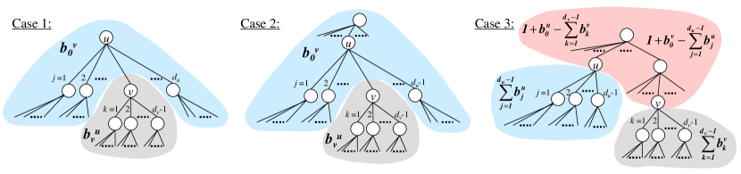
Figure 16: Centrality of high-degree nodes in the $s_{\max}$ tree.

Proof of Proposition 3: We proceed in two parts. First, we show that if node $v$ is downstream from node $u$, then $\bar{\sigma}(u)>\bar{\sigma}(v)$. Second, we show that if $v$ is in a different branch of the tree from $u$ (i.e., neither upstream nor downstream from $u$) but $d_{u}>d_{v}$, then $\bar{\sigma}(u)>\bar{\sigma}(v)$.

Starting first with the scenario where $v$ is downstream from $u$, there are two cases that need to be addressed.

Case 1: node $v$ is directly downstream from node $u$, and node $u$ is the root of the tree. Observe that we can represent $\bar{\sigma}(v)$ as

$$\bar{\sigma}(v) = b_{0}^{v}\sum_{k=1}^{d_{v}-1}b_{k}^{v}+\sum_{{j,k=1}\atop{j<k}}^{d_{v}-1}b_{j}^{v}b_{k}^{v}$$ (19)

$$= \bigg{(}\sum_{j=1\atop j\neq v}^{d_{u}}b_{j}^{u}\bigg{)}\bigg{(}b_{v}^{u}-1\bigg{)}+\sum_{j,k=1\atop j<k}^{d_{v}-1}b_{j}^{v}b_{k}^{v},\ \ \ \$$

since $b_{0}^{v}=\sum_{j=1;j\neq v}^{d_{u}}b_{j}^{u}$ and also that $b_{v}^{u}=1+\sum_{k=1}^{d_{v}-1}b_{k}^{v}$. For node $u$, we have

$$\bar{\sigma}(u) = \sum_{{j,k=1}\atop{j<k}}^{d_{u}}b_{j}^{u}b_{k}^{u}$$ (20)

$$= b_{v}^{u}\sum_{k=1\atop k\neq v}^{d_{u}}b_{k}^{u}+\sum_{j,k=1\atop j<k;j,k\neq v}^{d_{u}}b_{j}^{u}b_{k}^{u}.$$

Comparing $\bar{\sigma}(u)$ and $\bar{\sigma}(v)$, we observe that the first term of (20) is clearly greater than the first term of (19). Furthermore, by Lemma 1, we also observe that the second term of (20) is also greater than the second term of (19). Thus, we conclude for this case that $\bar{\sigma}(u)>\bar{\sigma}(v)$.

Case 2: node $v$ is directly downstream from node $u$, but node $u$ is not the root of the tree. Recognizing for any node $i$ that $\sum_{j=1}^{d_{i}-1}b_{j}=(n-1)-b_{0}$, we write

$$\bar{\sigma}(u) = b_{0}^{u}\big{(}n-1-b_{0}^{u}\big{)}+\sum_{j,k=1\atop j<k}^{d_{u}-1}b_{j}^{u}b_{k}^{u}$$

$$\bar{\sigma}(v) = b_{0}^{v}\big{(}n-1-b_{0}^{v}\big{)}+\sum_{j,k=1\atop j<k}^{d_{v}-1}b_{j}^{v}b_{k}^{v}$$

As before, we observe from Lemma 1 that $\sum_{j,k=1;j<k}^{d_{u}-1}b_{j}^{u}b_{k}^{u}>\sum_{j,k=1;j<k}^{d_{v}-1}b_{j}^{v}b_{k}^{v},$ so proving that $\bar{\sigma}(u)>\bar{\sigma}(v)$ in this case requires simply that we show

$$b_{0}^{u}\Big{(}(n-1)-b_{0}^{u}\Big{)}>b_{0}^{v}\Big{(}(n-1)-b_{0}^{v}\Big{)}.$$ (21)

Observe that $b_{0}^{v}=b_{0}^{u}+1+\sum_{j=1;j\neq v}^{d_{u}-1}b_{j}^{u}$. As a result, we have

$$b_{0}^{v}\Big{(}(n-1)-b_{0}^{v}\Big{)}$$

$$= \Big{(}b_{0}^{u}+1+\sum_{j=1\atop j\neq v}^{d_{u}-1}b_{j}^{u}\Big{)}$$

$$\Big{(}(n-1)-b_{0}^{u}-1-\sum_{j=1\atop j\neq v}^{d_{u}-1}b_{j}^{u}\Big{)}$$

$$= b_{0}^{u}\Big{(}(n-1)-b_{0}^{u}\Big{)}+\Big{(}1+\sum_{j=1\atop j\neq v}^{d_{u}-1}b_{j}^{u}\Big{)}$$

$$\bigg{(}(n-1)-2b_{0}^{u}-\Big{(}1+\sum_{j=1\atop j\neq v}^{d_{u}-1}b_{j}^{u}\Big{)}\bigg{)}$$

Since $1+\sum_{j=1;j\neq v}^{d_{u}-1}b_{j}^{u}>0$, (21) is true if and only if

$$(n-1)-2b_{0}^{u}-\Big{(}1+\sum_{j=1\atop j\neq v}^{d_{u}-1}b_{j}^{u}\Big{)} < 0$$

which is equivalent to

$$(n-1)-b_{0}^{u} < b_{0}^{u}+1+\sum_{j=1\atop j\neq v}^{d_{u}-1}b_{j}^{u}$$

$$\sum_{k=1}^{d_{u}-1}b_{k}^{u} < b_{0}^{u}+1+\sum_{j=1;j\neq v}^{d_{u}-1}b_{j}^{u}$$

$$b_{v}^{u} < b_{0}^{u}+1.$$

This final statement will always be true for the $s_{\max}$ tree, since the “upstream” branch from node $u$ will always contain at least as many nodes as the downstream branch corresponding to node $v$.

These two cases prove that any “upstream” node in the $s_{\max}$ tree is always more central than any “downstream” node, since by extension if $u$ is directly upstream from $v$ then $\bar{\sigma}(u)>\bar{\sigma}(v)$, and if $v$ is directly upstream from $w$ then $\bar{\sigma}(v)>\bar{\sigma}(w)$. It therefore follows that $\bar{\sigma}(u)>\bar{\sigma}(w)$, and, by induction, that the “root” node of the $s_{\max}$ tree (having highest degree) is the most central within the entire tree.

Case 3: Now we turn to the case where node $v$ is not directly downstream (or upstream) from node $u$. As before, we write

$$\bar{\sigma}(u) = b_{0}^{u}\sum_{k=1}^{d_{u}-1}b_{k}^{u}+\sum_{j,k=1;j<k}^{d_{u}-1}b_{j}^{u}b_{k}^{u},$$

$$\bar{\sigma}(v) = b_{0}^{v}\sum_{k=1}^{d_{v}-1}b_{k}^{v}+\sum_{j,k=1;j<k}^{d_{v}-1}b_{j}^{v}b_{k}^{v}.$$

As with the previous cases, by Lemma 1 we know that $\sum_{j,k=1;j<k}^{d_{u}-1}b_{j}^{u}b_{k}^{u}>\sum_{j,k=1;j<k}^{d_{v}-1}b_{j}^{v}b_{k}^{v},$ so proving that $\bar{\sigma}(u)>\bar{\sigma}(v)$ in this case requires simply that we show that

$$b_{0}^{u}\sum_{k=1}^{d_{u}-1}b_{k}^{u}>b_{0}^{v}\sum_{k=1}^{d_{v}-1}b_{k}^{v}.$$ (22)

We rewrite each of these as

$$b_{0}^{u} = \sum_{j=1}^{d_{v}-1}b_{j}^{v}+\Big{(}b_{0}^{u}-\sum_{j=1}^{d_{v}-1}b_{j}^{v}\Big{)}$$

$$b_{0}^{v} = \sum_{j=1}^{d_{u}-1}b_{j}^{u}+\Big{(}b_{0}^{v}-\sum_{j=1}^{d_{u}-1}b_{j}^{u}\Big{)}$$

so that we have

$$b_{0}^{u}\sum_{k=1}^{d_{u}-1}b_{k}^{u} = \bigg{(}\sum_{j=1}^{d_{v}-1}b_{j}^{v}+\Big{(}b_{0}^{u}-\sum_{j=1}^{d_{v}-1}b_{j}^{v}\Big{)}\bigg{)}\sum_{k=1}^{d_{u}-1}b_{k}^{u}$$

$$b_{0}^{v}\sum_{k=1}^{d_{v}-1}b_{k}^{v} = \bigg{(}\sum_{j=1}^{d_{u}-1}b_{j}^{u}+\Big{(}b_{0}^{v}-\sum_{j=1}^{d_{u}-1}b_{j}^{u}\Big{)}\bigg{)}\sum_{k=1}^{d_{v}-1}b_{k}^{v}$$

and observe that

$$b_{0}^{u}-\sum_{j=1}^{d_{v}-1}b_{j}^{v}=b_{0}^{v}-\sum_{j=1}^{d_{u}-1}b_{j}^{u},$$

which is a non-negative constant, that we denote $\kappa$. Thus,

$$b_{0}^{u}\sum_{j=1}^{d_{u}-1}b_{j}^{u}-b_{0}^{v}\sum_{j=1}^{d_{v}-1}b_{j}^{v} = \kappa\bigg{(}\sum_{j=1}^{d_{u}-1}b_{j}^{u}-\sum_{j=1}^{d_{v}-1}b_{j}^{v}\bigg{)},$$

which is also non-negative since $\sum_{j=1}^{d_{u}-1}b_{j}^{u}>\sum_{j=1}^{d_{v}-1}b_{j}^{v},$ and so (22) also holds. Thus, we have shown that $\bar{\sigma}(u)>\bar{\sigma}(v)$ in the $s_{\max}$ tree whenever $d_{u}>d_{v}$, thus completing the proof. ∎

Appendix B The $s(g)$-Metric and Assortativity

Following the development of Newman [73], let $P(\{D_{i}=k\})=P(k)$ be the node degree distribution over the ensemble of graphs and define $Q(k)=(k+1)P(k+1)/\sum_{j\in D}jP(j)$ to be the normalized distribution of remaining degree (i.e., the number of “additional” connections for each node at either end of the chosen link). Let $\bar{D}=\{d_{1}-1,d_{2}-2,\cdots,d_{n}-1\}$ denote the remaining degree sequence for $g$. This remaining degree distribution is $Q(k)=\sum_{k^{\prime}\in\bar{D}}Q(k,k^{\prime})$, where $Q(k,k^{\prime})$ is the joint probability distribution among remaining nodes, i.e., $Q(k,k^{\prime})=P(\{D_{i}=k+1,D_{j}=k^{\prime}+1|(i,j)\in\mathcal{E}\})$. In a network where the remaining degree of any two vertices is independent, i.e. $Q(k,k^{\prime})=Q(k)Q(k^{\prime})$, there is no degree-degree correlation, and this defines a network that is neither assortative nor disassortative (i.e., the “center” of this view into the ensemble). In contrast, a network with $Q(k,k^{\prime})=Q(k)\delta[k-k^{\prime}]$ defines a perfectly assortative network. Thus, graph assortivity $r$ is quantified by the average of $Q(k,k^{\prime})$ over all the links

$$r=\frac{\sum_{k,k^{\prime}\in\bar{D}}kk^{\prime}(Q(k,k^{\prime})-Q(k)Q(k^{\prime}))}{\sum_{k,k^{\prime}\in\bar{D}}kk^{\prime}(Q(k)\delta[k-k^{\prime}]-Q(k)Q(k^{\prime}))},$$ (23)

with proper centering and normalization according to the value of perfectly assortative network, which ensures that $-1\leq r\leq 1$. Many stochastic graph generation processes can be understood directly in terms of the correlation distributions among these so-called remaining nodes, and this functional form facilitates the direct calculation of their assortativity. In particular, Newman [73] shows that both Erdös-Renyí random graphs and Barabási-Albert preferential attachment growth processes yield ensembles with zero assortativity.

Newman [75] also develops the following sample-based definition of assortativity

$$r(g)=\frac{\left[\sum_{(i,j)\in\mathcal{E}}d_{i}d_{j}/l\right]-\left[\sum_{(i,j)\in\mathcal{E}}\frac{1}{2}(d_{i}+d_{j})/l\right]^{2}}{\left[\sum_{(i,j)\in\mathcal{E}}\frac{1}{2}(d_{i}^{2}+d_{j}^{2})/l\right]-\left[\sum_{(i,j)\in\mathcal{E}}\frac{1}{2}(d_{i}+d_{j})/l\right]^{2}},$$

which is equivalent to (14).

While the ensemble-based notion of assortativity in (23) has important differences from the sample-based notion of assortativity in (14), their relationship can be understood by viewing a given graph as a singleton on an ensemble of graphs (i.e., where the graph of interest is chosen with probability 1 from the ensemble). For this graph, if we define the number of nodes with degree $k$ as $N(k)$, we can derive the degree distribution $P(k)$ and the remaining degree distribution $Q(k)$ on the ensemble as

$$P(k)=\frac{N(k)}{n}$$

and

$$Q(k)=\frac{(k+1)P(k+1)}{\sum_{j\in D}jP(j)}=\frac{(k+1)N(k+1)}{\sum_{j\in D}jN(j)}.$$

Also it is easy to see that

$$\sum_{i\in\mathcal{V}}d_{i} = \sum_{k\in D}kN(k)=2l,$$

$$\sum_{i\in\mathcal{V}}d_{i}^{2} = \sum_{k\in D}k^{2}N(k),$$

$$\vdots$$

$$\sum_{i\in\mathcal{V}}d_{i}^{m} = \sum_{k\in D}k^{m}N(k),$$

where $m$ is a positive integer.

Equations (23) and (14) can be related term-by-term in the following manner. The first term of the numerator, $Q(k,k^{\prime})$, represents the joint probability distribution of the (remaining) degrees of the two nodes at either end of a randomly chosen link. For a given graph, let $l(k,k^{\prime})$ represent the number of links connecting nodes with degree $k$ to nodes with degree $k^{\prime}$. Then, we can write $Q(k,k^{\prime})=l(k,k^{\prime})/l$, and hence

$$\sum_{k,k^{\prime}\in\bar{D}}kk^{\prime}Q(k,k^{\prime})=\frac{1}{l}\sum_{(i,j)\in\mathcal{E}}d_{i}d_{j}.$$

The first term of the denominator of $r$ in equation (23) can be written as

$$\sum_{k,k^{\prime}\in\bar{D}}kk^{\prime}Q(k)\delta[k-k^{\prime}] = \sum_{k\in\bar{D}}k^{2}Q(k)$$

$$= \frac{\sum_{k\in D}(k+1)^{3}N(k+1)}{\sum_{i\in D}jN(j)}$$

$$= \frac{\sum_{i\in\mathcal{V}}d_{i}^{3}}{2l},$$ (25)

and the “centering” term (in both the numerator and the denominator) is

$$\sum_{k,k^{\prime}\in\bar{D}}kk^{\prime}Q(k)Q(k^{\prime}) = \left(\sum_{k\in\bar{D}}kQ(k)\right)^{2}$$

$$= \left(\frac{\sum_{k\in D}(k+1)^{2}N(k+1)}{\sum_{i\in D}jN(j)}\right)^{2}$$

$$= \left(\frac{\sum_{i\in\mathcal{V}}d_{i}^{2}}{2l}\right)^{2}.$$ (27)

In both of these cases, the offset of a constant in representing the degree sequence as $D$ versus $\bar{D}$ does not effect the overall calculation. The relationships between the ensemble-based quantities (LHS of B) and (LHS of B) and their sample-based (i.e., structural) counterparts (25) and (27) holds (approximately) when the expected degree equals the actual degree.

To see why (27) can be viewed as the “center”, we consider the following thought experiment: what is the structure of a deterministic graph with degree sequence $D$ and having zero assortativity? In principle, a node in such a graph will connect to any other node in proportion to each node’s degree. While such a graph may not exist for general $D$, one can construct a deterministic pseudograph $\tilde{g}$ having zero assortativity in the following manner. Let $A=[a_{ij}]$ represent a (directed) node adjacency matrix of non-negative real values, representing the “link weights” in the pseudograph. That is, links are not constrained to integer values but can exist in fractional form. The zero assortative pseudograph will have symmetric weights given by

$$a_{ij}=\left(\frac{d_{j}}{\sum_{k\in\mathcal{V}}d_{k}}\right)\left(\frac{d_{i}}{2}\right)=\left(\frac{d_{i}}{\sum_{k\in\mathcal{V}}d_{k}}\right)\left(\frac{d_{j}}{2}\right)=a_{ji}.$$

Thus, the weight $a_{ij}$ for each link emanating out of node $i$ is in proportion to the degree of node $j$, in a manner that is relative to the sum of all node degrees. In general, the graphs of interest to us are undirected, however here it is notationally convenient to consider the construction of directed graphs. Using these weights, the total weight among all links entering and exiting a particular node $i$ equals

$$\sum_{j\in\mathcal{V}}a_{ij}+\sum_{k\in\mathcal{V}}a_{ki}=d_{i}/2+d_{i}/2=d_{i}.$$

Accordingly, the total “link weights” in the pseudograph are equal to

$$\sum_{i,j\in\mathcal{V}}a_{ij}=\sum_{j\in\mathcal{V}}d_{j}/2=l,$$

where $l$ corresponds to the total number of links in a traditional graph. The $s$-metric for the pseudograph $\tilde{g}_{A}$ represented by matrix $A$ can be calculated as

$$s(\tilde{g}_{A}) = \sum_{j\in\mathcal{V}}\sum_{i\in\mathcal{V}}d_{i}a_{ij}d_{j}$$

$$= \sum_{j\in\mathcal{V}}\left[\sum_{i\in\mathcal{V}}d_{i}\left(\frac{d_{j}}{\sum_{k\in\mathcal{V}}d_{k}}\right)\left(\frac{d_{i}}{2}\right)\right]d_{j}$$

$$= \frac{\Big{(}\sum_{j\in\mathcal{V}}d_{j}^{2}\Big{)}\Big{(}\sum_{i\in\mathcal{V}}d_{i}^{2}\Big{)}}{2\Big{(}\sum_{k\in\mathcal{V}}d_{k}\Big{)}}$$

$$= \frac{\Big{(}\sum_{j\in\mathcal{V}}d_{j}^{2}\Big{)}^{2}}{4l},$$

and we have

$$\frac{s(\tilde{g}_{A})}{l} = \left(\frac{\sum_{i\in\mathcal{V}}d_{i}^{2}}{2l}\right)^{2},$$

which is equal to (27).

In principle, one could imagine a deterministic procedure that uses the structural pseudograph $\tilde{g}_{A}$ to generate the zero assortativity graph among an “unconstrained” background set $G$. That is, graphs resulting from this procedure could have multiple links between any pair of nodes as well as multiple self-loops and would not necessarily be connected. The challenge in developing such a procedure is to ensure that the resulting graph has degree sequence equal to $D$, although one can imagine that in the limit of large graphs this becomes less of an issue. By extension, it is not hard to conceive a stochastic process that uses the structural pseudograph $\tilde{g}_{A}$ to generate a statistical ensemble of graphs having expected assortativity equal to zero. In fact, it is not hard to see why the GRG method is very close to such a procedure.

Note that the total weight in the pseudograph between nodes $i$ and $j$ equals $a_{ij}+a_{ji}=d_{i}d_{j}/2l$. Recall from Section 5.1 that the GRG method described is based on the choice of a probability $p_{ij}=\rho d_{i}d_{j}$ of connecting two nodes $i$ and $j$, and also that in order to ensure that $E(d_{i})=d_{i}$ one needs $\rho=1/2l$, provided that $\max_{i\neq j\in\mathcal{V}}d_{i}d_{j}\leq 2l$. Thus, the GRG method can be viewed as a stochastic procedure that generates real graphs from the pseudograph $\tilde{g}_{A}$, with the one important difference that the GRG method always results in simple (but not necessarily connected) graphs. Thus, the zero assortativity pseudograph $\tilde{g}_{A}$ can be interpreted as the “deterministic outcome” of a GRG-like construction method. Accordingly, one expects that the statistical ensemble of graphs resulting from the stochastic GRG method could have zero assortativity, but this has not been proven.

In summary, graph assortativity captures a fundamental feature of graph structure, one that is closely related to our $s$-metric. However, the existing notion of assortativity for an individual graph $g$ is implicitly measured against a background set of graphs $G$ that is not constrained to be either simple or connected. The connection between the sample-based and ensemble-based definitions makes it possible to calculate the assortativity among graphs of different sizes and having different degree sequences, as well as for different graph evolution procedures. Unfortunately, because this metric is computed relative to an unconstrained background set, in some cases this normalization (against the $s_{\max}$ graph) and centering (against the $\tilde{g}_{A}$ pseudograph) does a relatively poor job of distinguishing among graphs having the same degree sequence, such as those in Figure 5.

References

- [1] D. Achlioptas, A. Clauset, D. Kempe, and C. Moore On the bias of traceroute sampling; or, power-law degree distributions in regular graphs. 2003. cond-mat/0503087
- [2] W. Aiello, F. Chung, and L. Lu. A Random Graph Model for Massive Graphs. Proc. STOC 2000.
- [3] W. Aiello, F. Chung, and L. Lu. Random evolution in massive graphs. In: Handbook on Massive Data Sets, (Eds. J. Abello et al.), pp. 97–122, 2001.
- [4] R. Albert and A-L. Barabási. Statistical mechanics of complex networks. Reviews of Modern Physics, Vol. 74, January 2002.
- [5] R. Albert, H. Jeong, and A.-L. Barabási. Diameter of the World Wide Web, Nature 401, 130-131 (1999)
- [6] R. Albert, H. Jeong, and A.-L. Barabási. Attack and error tolerance of complex networks, Nature 406, 378-382 (2000)
- [7] D. Alderson. Technological and Economic Drivers and Constraints in the Internet’s “Last Mile”, Tech Report CIT-CDS-04-004, California Institute of Technology (2004)
- [8] D. Alderson and W. Willinger. A contrasting look at self-organization in the Internet and next-generation communication networks. IEEE Communications Magazine, July 2005.
- [9] L.A.N. Amaral, A. Scala, M. Barthelemy, and H.E. Stanley. Classes of small-world networks. Proc. Natl. Acad. Sci. USA 97:11149–11152, 2000.
- [10] M. Arita. The metabolic world of Escherichia coli is not small. PNAS, Vol. 101, No. 6, 1543–1547, February 10, 2004.
- [11] P. Bak How nature works: the science of self-organized criticality, Copernicus (1996)
- [12] P. Ball. Critical Mass: How One Thing Leads to Another. Farrar, Straus and Giroux (2004).
- [13] P. Ball. Networking can be hazardous, Nature Science Update, 9 March 2001.
- [14] A.-L. Barabási Linked: The New Science of Networks. Perseus Publishing(2002)
- [15] A.-L. Barabási and R. Albert. Emergence of scaling in random networks, Science 286, 509-512 (1999)
- [16] A.-L. Barabási, R. Albert, and H. Jeong Mean-field theory for scale-free random networks, Physica A 272, 173-187 (1999)
- [17] A.-L. Barabási and E. Bonabeau. Scale-Free Networks. Scientific American 288, 60-69 (2003).
- [18] A.-L.Barabási, Z. Dezso, E. Ravasz, S.H.Yook, and Z. Oltvai. Scale-free and Hierarchical Structures in Complex Networks, AIP Conference Proceedings, 2003.
- [19] A.-L. Barabási and Z.N. Oltvai. Network biology: understanding the cell’s functional organization. Nature Reviews Genetics 5, 101–114 (2004).
- [20] A.-L. Barabási, E. Ravasz, and T. Vicsek. Deterministic scale-free networks. Physica A 2001; 299:599, cond-mat/0107419.
- [21] N. Berger, C. Borgs, J. Chayes and A. Saberi. On the Spread of Viruses on the Internet. ACM-SIAM Symposium on Discrete Algorithms (SODA05) Vancouver, British Columbia, January 23-25, 2005.
- [22] G. Bianconi and A.-L. Barabási Competition and Multiscaling in Evolving Networks, Europhys. Lett. 54, 436-442 (2001)
- [23] B. Bollobas Modern Graph Theory. Springer 1998.
- [24] B. Bollobás and O. Riordan. Robustness and vulnerability of scale-free random graphs, Internet Math. 1, pp. 1–35, 2003.
- [25] B. Bollobás and O. Riordan. The Diameter of a Scale-Free Random Graph, Combinatorica 24(1), pp. 5–34, 2004.
- [26] L. Briesemeister, P. Lincoln, and P. Porras, Epidemic Profiles and Defense of Scale Free Networks. ACM Workshop on Rapid Malcode (WORM), Washington, D.C. October 27, 2003.
- [27] M. Buchanan. Ubiquity: The Science of History…or Why the World Is Simpler Than We Think. Crown. 2001.
- [28] J. M. Carlson and J. C. Doyle. Highly Optimized Tolerance: a mechanism for power laws in designed systems. Physics Review E, 60:1412–1428, 1999.
- [29] J.M. Carlson and J.Doyle Complexity and Robustness PNAS, 99, Suppl. 1, 2539-2545 (2002)
- [30] H. Chang, R. Govindan, S. Jamin, S. Shenker, and W. Willinger. Towards Capturing Representative AS-Level Internet Topologies ACM SIGMETRICS 2002 (2002).
- [31] G. Chartrand, G. Kubicki, and M. Schultz. Graph similarity and distance in graphs. Aequationes Mathematicae, Vol. 55, pp. 129–145, 1998.
- [32] F. Chung and L. Lu. The average distance in a random graph with given expected degrees, Internet Math., 1: 91–113, 2003.
- [33] D. D. Clark. The design philosophy of the DARPA Internet protocols. Proc. of the ACM SIGCOMM’88, in: ACM Computer Communication Reviews, Vol. 18, No. 4, pp. 106–114, 1988.
- [34] Cooperative Association for Internet Data Analysis (CAIDA), Skitter. Available at http://www.caida.org/ tools/measurement/skitter/.
- [35] M.E. Csete and J.C. Doyle. Reverse engineering of biological complexity, Science 295, 1664 (2002).
- [36] M. Csete and J. Doyle. Bowties, metabolism, and disease, Trends in Biotechnology, 22, 446-450 (2004).
- [37] Z. Dezsö and A.-L. Barabási, Halting viruses in scale-free networks, Physical Review E (2002)
- [38] S. Dill, R. Kumar, K. McCurley, S. Rajagopalan, D. Sivakumar, and A. Tompkins. Self-similarity in the Web. ACM Trans. Internet Technology, Vol. 2, pp. 205–223, 2002.
- [39] P.S. Dodds and D.H. Rothman. Unified view of scaling laws in river networks. Phys. Rev. E, 59(5):4865–4877, 1999.
- [40] S. N. Dorogovtsev and J. F. F. Mendes. Evolution of Networks: From Biological Nets to the Internet and WWW. Oxford University Press, Oxford, UK, 2003.
- [41] J.C. Doyle, D. Alderson, L. Li, S. Low, M. Roughan, S. Shalunov, R. Tanaka, and W. Willinger. The “Robust Yet Fragile” Nature of the Internet. Proc. Natl. Acad. Sci. USA 102(41). 2005.
- [42] P. Erdös and T. Gallai. Graphs with prescribed degrees of vertices. Mat. Lapok (Hungarian), 11:264-274, 1960.
- [43] P. Erdos and A. Renyi. On random graphs I Publ. Math. (Debrecen) 9 (1959), 290-297.
- [44] A. Fabrikant, E. Koutsoupias, and C. Papadimitriou. (2002) Heuristically Optimized Trade-offs: A new paradigm for Power- laws in the Internet, Proceedings of ICALP 2002; 110–122.
- [45] S.M. Fall. Galaxy correlations and cosmology. Reviews of Modern Physics 51(1):21–42, 1979.
- [46] I. Farkas, I. Der nyi, G. Palla, and T. Vicsek. Equilibrium statistical mechanics of network structures Springer-Verlag Lect. Notes in Phys. 650:163-187 (2004)
- [47] W. Feller. An Introduction to Probability Theory and Its Applications, Volume 2. John Wiley & Sons. New York. 1971.
- [48] E. Fox Keller. Revisiting “scale-free” networks. BioEssays 27.10:1060–1068 (2005).
- [49] C. Gkantsidis, M. Mihail, and E. Zegura. The markov chain simulation method for generating connected power law random graphs. Proc. 5th Workshop on Algorithm Engineering and Experiments (SIAM Alenex’03), 2003.
- [50] R. Govindan and H. Tangmunarunkit. Heuristics for Internet Map Discovery, IEEE INFOCOM 2000.
- [51] E.J. Groth and P.J.E. Peebles. The Large Scale Structure of the Universe, Astrophysics Journal, vol.217, p.385, 1977.
- [52] J.T. Hack. Studies of longitudinal stream profiles in Virginia and Maryland. US Geol. Survey Prof. Paper, Vol. 294-B, pp. 45–94, 1957.
- [53] R.E. Horton. Erosional development of streams and their drainage basins: Hydrophysical approach to quantitative morphology. Bull. Geol. Soc. America, Vol. 56, pp. 275–370, 1945.
- [54] H. Jeong, S.P. Mason, A.-L. Barabási, Z.N. Oltvai. Lethality and centrality in protein networks. Nature 411, 41-42 (2001).
- [55] H.Jeong, B. Tombor, R. Albert, Z. N. Oltvai and A-L Barab si The large-scale organization of metabolic networks, Nature 407, 651 (2000)
- [56] H. Jeong, Z. Neda, and A-L. Barabási. Measuring Preferential Attachment in Evolving Networks, Europhys. Letter 61, 567-572 (2003)
- [57] Johnson, N.L., S. Kotz, and N. Balakrishnan. Continuous Univariate Distributions. Vol. 1, 2nd Ed. New York: John Wiley & Sons. 1994.
- [58] S. Itzkovitz, R. Levitt, N. Kashtan, R. Milo, M. Itzkovitz, and U. Alon. Coarse-Graining and Self-Dissimilarity of Complex Networks. arXiv:q-bio.MN/0405011 v1, 14 May 2004.
- [59] S. Itzkovitz, R. Levit, N. Kashtan, R. Milo, M. Itzkovitz, and U. Alon. Multi-Level Coarse-Graining of Complex Networks. Preprint.
- [60] J.W. Kirchner. Statistical inevitability of Horton’s laws and the apparent randomness of stream channel networks. Geology, vol. 21, pp. 591–594, July 1993.
- [61] J.W. Kirchner. Statistical inevitability of Horton’s laws and the apparent randomness of stream channel networks–Reply to Masek and Turcotte. Geology, 22: 380–381, April 1994.
- [62] J.W. Kirchner. Statistical inevitability of Horton’s laws and the apparent randomness of stream channel networks–Reply to Troutman and Karlinger, Geology, 22: 574–575, June 1994.
- [63] H.-P. Kriegel and S. Schonauer. Similarity search in structured data. Proc. 5th Conf. on Data Warehousing and Knowledge Discovery DaWaK’03, Prague, Czech Republic, 2003.
- [64] A. Lakhina, J.W. Byers, M. Crovella, and P. Xie. Sampling Biases in IP topology Measurements, IEEE INFOCOM 2003.
- [65] L. Li, D. Alderson, J. Doyle, and W. Willinger. A First-Principles Approach to Understanding the Internet’s Router-level Topology. Proc. ACM SIGCOMM 2004.
- [66] S.E. Luria and M. Delbrück. Mutations of bacteria from virus sensitivity to virus resistance. Genetics, vol. 28, 491–511, 1943.
- [67] B.B. Mandelbrot. Fractals and Scaling in Finance: Discontinuity, Concentration, Risk. Springer-Verlag, New York, 1997.
- [68] A. Marani, R. Rigon, and A. Rinaldo. A note on fractal channel networks. Water Resources Research, Vol. 27, No. 12, pp. 3041–3049, 1991.
- [69] Matlab code for generating the sequences used in Figure 1 is available from http://hot.caltech.edu/topology/RankVsFreq.m.
- [70] R. Milo, S. Shen-Orr, S. Itzkovitz, N. Kashtan, D. Chklovskii, and U. Alon. Network Motifs: Simple Building Blocks of Complex Networks. Science, 298 (2002).
- [71] M. Mitzenmacher. A Brief History of Generative Models for Power Law and Lognormal Distributions, Internet Math. 1(2):226-251, 2004.
- [72] M.E.J. Newman. A measure of betweenness centrality based on random walks. Social Networks 27, 39–54, 2005.
- [73] M.E.J. Newman Assortative Mixing in Networks, Phys. Rev. Lett. 89, 208701 (2002)
- [74] M.E.J. Newman. The Structure and Function of Complex Networks, SIAM Review 45, 167-256 (2003)
- [75] M.E.J. Newman. Power laws, Pareto distributions and Zipfs law, Contemporary Physics, in press. (Available electronically from arXiv:cond-mat/0412004, January 2005)
- [76] J. Ottino. Engineering Complex Systems. Nature 427 (29), January 2004.
- [77] J. Park and M.E.J.Newman The origin of degree correlations in the Internet and other networks Phys. Rev. E. 68, 026112, 2003.
- [78] R. Pastor-Satorras and A. Vespignani. Epidemic spreading in scale-free networks Physical Review Letters, 86(14), pp. 3200–3203, April 2, 2001.
- [79] R. Pastor-Satorras and A. Vespignani. Evolution and Structure of the Internet : A Statistical Physics Approach. Cambridge University Press, Cambridge, UK, 2004.
- [80] K. Patch. Net inherently virus prone, Technology Research News, March 21, 2001.
- [81] V. Paxson. Strategies for Sound Internet Measurement. Proc. ACM SIGCOMM Internet Measurement Conference IMC 2004 (2004).
- [82] S.D. Peckham. New results for self-similar tree with applications to river networks. Water Resources Research, vol. 31, no. 4, pp. 1023–1029, April 1995.
- [83] E. Petrakis. Design and evaluation of spatial similarity approaches for image retrieval. Image and Vision COmputing, Vol. 20, pp. 59–76, 2002.
- [84] E. Ravasz, A.L. Somera, D.A. Mongru, Z.N. Oltvai, and A.-L. Barabási. Hierarchical organization of modularity in metabolic networks, Science, 2002.
- [85] S. I. Resnick. Heavy tail modeling and teletraffic data. Annals of Statistics 25, pp. 1805–1869, 1997.
- [86] A. Rinaldo, I. Rodríguez-Iturbe, R. Rigon, R.L. Bras, E. Ijjász-Vásquez, and A. Marani. Minimum Energy and Fractal Structures of Drainage Networks, Water Resources Research 28(9):2183-2195, 1992.
- [87] I. Rodríguez-Iturbe, A. Rinaldo, R. Rigon, R.L. Bras, A. Marani, and E. Ijjász-Vásquez. Energy Dissipation, Runoff Production, and the Three-Dimensional Structure of River Basins, Water Resources Research 28(4):1095-1103, 1992.
- [88] Route Views, University of Oregon Route Views Project, http://www.antc.uoregon.edu/route-views/.
- [89] G. Samorodnitsky, and M.S. Taqqu. Stable Non-Gaussian Random Processes: Stochastic Models with Infinite Variance. Chapman and Hall, New York - London, 1994.
- [90] A. Sanfeliu and K.S. Fu. A distance measure between attributed relational graph. IEEE Trans. Systems, Man and Cybernetics, Vol. 13, pp. 353–362, 1983.
- [91] T. Seidl. References for graph similarity. http://www.dbs. informatik.uni-muenchen.de/ seidl/graphs/.
- [92] S.S. Shen-Orr, R. Milo, S. Mangan, et al. Network motifs in the transcriptional regulation network of Escherichia coli. Nature Genetics, 31 (1): 64–68, May 2002.
- [93] S.S. Skiena. The Algorithm Design Manual. New York: Springer-Verlag, 1997. Available electronically from http://www2.toki.or.id/book/AlgDesignManual/.
- [94] H.A. Simon On a class of skew distribution functions. Biometrika, Vol. 42, No. 3/4, 425-440 (1955).
- [95] N. Spring, M. Dontcheva, M. Rodrig, and D. Wetherall. How to Resolve IP Aliases, UW CSE Tech. Report 04-05-04, 2004.
- [96] N. Spring, R. Mahajan, D. Wetherall, and T. Anderson. Measuring ISP Topologies with Rocketfuel, IEEE/ACM Transactions on Networking, Vol. 12, pp. 2–16 (2004).
- [97] R. Solé and S. Valverde, Information Transfer and Phase Transitions in a model of Internet Traffic, Physica A 289 (2001), 595-695
- [98] D. Stauffer and A. Aharony. Introduction to Percolation Theory, 2nd edition. Taylor and Francis, London, 1992.
- [99] J. Stelling, U. Sauer, Z. Szallasi, F.J. Doyle, and J. Doyle Robustness of cellular functions. Cell, Vol. 118, pp. 675–685, 2004.
- [100] J. W. Stewart III. BGP4: Inter-Domain Routing in the Internet. Addison-Wesley, Boston, 1999.
- [101] A.N. Strahler. Quantitative analysis of watershed geomorphology. Trans. Am. Geophy. Union, 38(6):913–920, 1957.
- [102] R. Tanaka. Scale-rich metabolic networks. Physical Review Letters 94, 168101 (2005)
- [103] R. Tanaka, M. Csete and J. Doyle. Global organization of metabolic networks: Implications for complex biologic systems, in preparation.
- [104] R. Tanaka, M. Csete and J. Doyle. Highly optimized global organization of metabolic networks. IEE Proc. Systems Biology, in press (2005).
- [105] R. Tanaka, T.-M. Yi and J. Doyle. Some protein interaction data do not exhibit power law statistics, FEBS letters 579, 5140-5144 (2005).
- [106] D.G. Tarboton. Fractal river networks, Horton’s laws, and Tokunaga cyclicity. Hydrology, Vol. 187, pp. 105–117, 1996.
- [107] R. Teixeira, K. Marzullo, S. Savage, and G.M. Voelker. In Search of Path Diversity in ISP Networks, In Proc. IMC’03, Miami Beach, Florida. October 27-29, 2003.
- [108] A. Tripathi and S. Vijay. A note on a theorem of Erdös & Gallai. Discrete Mathematics Volume 265, Issue 1-3, 2003.
- [109] D.J. Watts and S.H. Strogatz. Collective dynamics of “small world” networks. Nature, Vol. 393, June 1998.
- [110] W. Willinger, D. Alderson, J. Doyle, and L. Li. A pragmatic approach to dealing with high variability in network measurements. Proc. ACM SIGCOMM Internet Measurement Conference IMC 2004 (2004).
- [111] W. Willinger, D. Alderson, J.C. Doyle, and L.Li. More “Normal” Than Normal: Scaling Distributions and Complex Systems. Proceedings of the 2004 Winter Simulation Conference R.G. Ingalls, M.D. Rossetti, J.S. Smith, and B.A. Peters, eds. (2004)
- [112] D.H. Wolpert and W. Macready. Self-dissimilarity: An empirically observable complexity measure, Unifying Themes in Complex Systems, New England Complex Systems Institute, 626–643 (2000)
- [113] D.H. Wolpert and W. Macready. Self-dissimilarity as a high dimensional complexity measure. Preprint, 2004.
- [114] K.Wu and A. Liu The Rearrangement Inequality, http:// matholymp.com/TUTORIALS/Rear.pdf
- [115] S.-H. Yook, H. Jeong, and A.-L. Barabási. Modeling the Internets large-scale topology, PNAS 99, 13382-13386 (2002)
- [116] S.-H. Yook, Z.N. Oltvai and A.-L. Barabási. Functional and topological characterization of protein interaction networks. Proteomics 4, 928-942 (2004).
- [117] G. Yule. A mathematical theory of evolution based on the conclusions of Dr. J.C. Willis F.R.S. Philosophical Transactions of the Royal Society of London (Series B), 213, 21-87 (1925).
- [118] Y. Zhang, M. Roughan, C. Lund, and D. Donoho. An information-theoretic approach to traffic matrix estimation. Proc. ACM SIGCOMM 2003.