Dielectric resonances of ordered passive arrays

Abstract

The electrical and optical properties of ordered passive arrays, constituted of inductive and capacitive components, are usually deduced from Kirchhoff’s rules. Under the assumption of periodic boundary conditions, comparable results may be obtained via an approach employing transfer matrices. In particular, resonances in the dielectric spectrum are demonstrated to occur if all eigenvalues of the transfer matrix of the entire array are unity. The latter condition, which is shown to be equivalent to the habitual definition of a resonance in impedance for an array between electrodes, allows for a convenient and accurate determination of the resonance frequencies, and may thus be used as a tool for the design of materials with a specific dielectric response. For the opposite case of linear arrays in a large network, where periodic boundary condition do not apply, several asymptotic properties are derived. Throughout the article, the derived analytic results are compared to numerical models, based on either Exact Numerical Renormalisation or the spectral method.

1 Introduction

Recent experimental advances Pendry2004 have put to living the speculation about materials with negative refraction index, initiated in 1968 by Victor Veselago on purely theoretical grounds Veselago1968 . Such materials, starting to be at reach nowadays primarily for the microwave region, manifest exciting and unconventional phenomena ranging from the Inverse Doppler effect Seddon2003 to the possibility of diffraction-free imaging Grbic2004 .

Were such “left-handed” materials, as Veselago called them, available for any frequency domain, they would undoubtedly revolutionise optics. However, a negative refraction index requires simultaneously a negative permittivity and a negative permeability, implying that the material has dielectric and magnetic resonances in the same frequency domain — a property which turns out to be extremely rare and which is partly responsible why such materials have remained undiscovered for almost three decades.

Unlike to the optical domain, where the electric and magnetic resonances are generally separated in frequency by several orders of magnitude, negatively refracting materials have recently been engineered for narrow bands in the microwave domain. One of the main ingredients of these “metamaterials” are regular arrays of so-called split-ring resonators Pendry2004 .

In this paper, we will focus on the dielectric part of the response of arrays of similar resonators in square lattices. One goal is to provide tools for the location of the resonances in the spectrum, a task which cannot simply be performed by looking at the building blocks of such an array Laurent2003 . At the same time, the theoretical approaches presented in this paper allow for a deeper understanding of the resonance spectrum — certainly an advantage in the quest of materials with a tailored electromagnetic response. Throughout the paper, the analytical results are compared to numerically calculated spectra, obtained either via Exact Numerical Renormalisation (ENR) Vinograd ; Sarych ; Tort or from the spectral method Straley ; Bergman ; Milton formulated with Green’s functions Clerc1996 ; Luck1998 ; Laurent2000 .

An archetype of the circuits to be dealt with in this paper is depicted in Fig. 1.

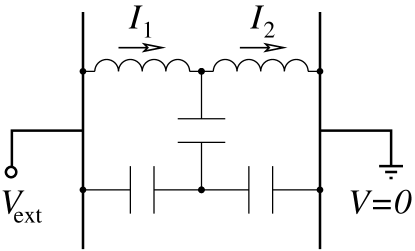
Figure 1: One of the simplest non-trivial clusters, consisting of two self-induction coils embedded in a capacitor network.

This “cluster” consists of two coils in series (each of inductance $L$ and with no ohmic resistance, $R=0$) embedded in the simplest imaginable network made of three capacitors (each of capacity $C$). As will be seen in the following, this circuit contains — despite its simplicity — many of the essential features of the more complicated arrays to be studied in the following sections.

With no external voltage applied to the plates, the state of the system can be obtained by straightforward application of Kirchhoff’s rules: the loop rule yields a differential equation for the current through any of the coils $I_{k}$ in terms of the currents flowing through the vertical and the horizontal capacitor belonging to the same loop; the latter currents are subsequently eliminated by Kirchhoff’s junction rule, resulting in a homogeneous system of two ordinary differential equations for the currents through the coils. Applying a time-dependent external voltage $V_{\rm ext}(t)$ to the plates introduces an inhomogeneity in the equations, which finally read

$$\frac{1}{\omega_{0}^{2}}\frac{\mathrm{d}^{2}}{\mathrm{d}t^{2}}\begin{pmatrix}I_{1}\\ I_{2}\end{pmatrix}\,-\,\begin{pmatrix}-2&\;1\\ \;1&-2\end{pmatrix}\begin{pmatrix}I_{1}\\ I_{2}\end{pmatrix}\;=\;I_{\rm ext}(t)\begin{pmatrix}1\\ 1\end{pmatrix}\text{,}$$ (1)

with $\omega_{0}=1/\sqrt{LC}$ and $I_{\rm ext}(t)$ the total net current flowing through the sample.

Eq. (1) can be solved by standard means yielding the homogeneous eigenmodes

$$\mathbf{I}_{\rm h}(t)\;=\;c_{1}\begin{pmatrix}1\\ 1\end{pmatrix}\mathrm{e}^{\mathrm{i}\omega_{0}t}\,+\,c_{2}\begin{pmatrix}\;1\\ -1\end{pmatrix}\mathrm{e}^{\mathrm{i}\sqrt{3}\omega_{0}t}\;\mbox{,}$$ (2)

where $c_{1}$ and $c_{2}$ are arbitrary complex amplitudes. The application of a sinusoidal external voltage of frequency $\Omega$, implying an external current $I_{\rm ext}(t)=\hat{I}_{\rm ext}\exp(\mathrm{i}\Omega t)$, allows for one additional solution

$$\mathbf{I}_{\rm inh}(t)\;=\;I_{\rm ext}(t)\begin{pmatrix}1\\ 1\end{pmatrix}\,\begin{cases}\frac{\omega_{0}^{2}}{\omega_{0}^{2}-\Omega^{2}}&\text{for $\Omega\neq\omega_{0}$, }\\ -\frac{\mathrm{i}}{2}\omega_{0}t&\text{for $\Omega=\omega_{0}$.}\end{cases}$$ (3)

Four observations can be made at this point: (i) in networks consisting of two species of components only, the state of the system is fully described by a set of differential equations for the currents flowing through the minority components (in our case the coils). The contribution of the majority components (here, the capacitors) to the Kirchhoff rules is purely algebraic, and may be eliminated from the system of equations. (ii) The external voltage can only excite the first resonance, of frequency $\omega_{0}$. The second resonance, $\sqrt{3}\omega_{0}$, is antisymmetric ($I_{1}=-I_{2}$) and thus orthogonal to the currents which are always induced symmetrically in the present configuration of the voltage plates. (iii) The applied voltage equals the sum of the two voltage drops in the coils, i.e. $V_{\rm ext}=L\frac{\mathrm{d}}{\mathrm{d}t}(I_{1}+I_{2})$. Off resonance, this yields a total impedance of $Z={V_{\rm ext}}/{I_{\rm ext}}=2\mathrm{i}L\Omega\omega_{0}^{2}/(\omega_{0}^{2}-\Omega^{2})$ between the plates. This result may be generalised: as a resonance is approached, the internal currents of the sample diverge for finite applied voltage. This may be associated with an infinite conductivity of the sample’s (internal) components. At the same time, however, a divergent impedance and thus zero conductivity is measured between the plates. (iv) In reality, the coils have a small but finite ohmic resistance $R$. The eigenfrequencies are thus shifted slightly in the complex plane towards small positive imaginary parts which damp out the sample’s free modes, eq. (2). In addition to its imaginary part, the impedance $Z$ acquires a real part consisting of a narrow lorentzian peak centred at the resonance frequency.

The paper is organised as follows: in Sec. 2, the resonance spectra of regular arrays with not too complicated unit cells are calculated directly from the solution of Kirchhoff’s rules. In Sec. 3, more complicated arrays are tackled with an approach based on transfer matrices. Regular one-dimensional (1D) arrays in an infinite two-dimensional (2D) lattice are examined in Sec. 4, and the results compared to the formerly discussed 2D clusters. Finally, the Appendix A is devoted to a simple physical approximation, based on a dipole scenario in a 2D environment, which turns out to be helpful for the interpretation of the spectra of linear clusters.

2 Direct solution of Kirchhoff’s rules

In this section, we will tackle simple regular 1D and 2D binary arrays by a direct solution of Kirchhoff’s rules. The results are then to be compared to those obtained by Exact Numerical Renormalisation (ENR) Vinograd ; Sarych ; Tort . The strategy of the latter algorithm consists of eliminating the network sites one by one, while renormalising the impedance between all couples of former neighbours of the eliminated site such that the global impedance remains invariant, until the electrodes are connected by just one bond, which then carries the whole network’s impedance.

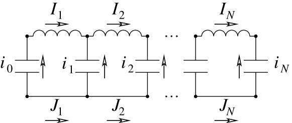
Figure 2: A ladder-shaped circuit containing $N$ coils in series on one leg, and the same number of bonds with no impedance on the other. All $N+1$ steps of the ladder are capacitors.

To begin with, we are going to summarise the solution of Kirchhoff’s rules for the 1D array shown in Fig. 2. This ladder-shaped circuit consists of a horizontal line of $N$ coils, each of inductance $L$, which is connected by $N+1$ capacitors, each of capacity $C$, to another horizontal line with no resistance at all. The loop rule states that the voltage drop around a closed loop is zero; applying it to the $k.$th mesh and deriving with respect to time yields ${\mathrm{d}^{2}I_{k}}/{\mathrm{d}t^{2}}=\omega_{0}^{2}(i_{k}-i_{k-1})$, with $\omega_{0}=1/\sqrt{LC}$. The currents through the capacitors, $i_{k}$, can be eliminated using the junction rule $i_{k}+I_{k}=I_{k+1}$, where $I_{k}$ is assumed zero if $k$ is out of range. In total, we get

$$\frac{\mathrm{d}^{2}}{\mathrm{d}t^{2}}\mathbf{I}\;=\;\omega_{0}^{2}\mathbf{D}\mathbf{I}\text{,}$$ (4)

where ${\mathbf{I}=(I_{1},\ldots,I_{N})}^{\mathrm{T}}$ is the coil current vector, and $\mathbf{D}$ the 1D lattice Laplacian, i.e. a tridiagonal matrix with entries $-2$ for all diagonal elements and $1$ for all non-zero off-diagonal elements.

The usual ansatz $\mathbf{I}\sim\exp{(\mathrm{i}\omega t)}$ converts the differential equation (4) into an eigenvalue problem for the tridiagonal matrix $\mathbf{D}+\tilde{\omega}^{2}\mathbf{1}$, where $\tilde{\omega}=\omega/\omega_{0}$ stands for the frequency in units of $\omega_{0}$. Its determinant can be calculated explicitly: for a $N$-dimensional tridiagonal matrix $\mathbf{M}_{N}(x)$ with diagonal elements $2x$, and first sub- and super-diagonal elements $1$, expansion of the determinant by minors yields

$$D_{N}(x)\;=\;2xD_{N-1}(x)\,-\,D_{N-2}(x)\;\text{,}$$ (5)

where $D_{N}(x)=\det{\mathbf{M}_{N}(x)}$. We recognise in (5) the recurrence relation generating the Chebyshev polynomials. The required initial conditions, $D_{0}(x)=1$ and $D_{1}(x)=2x$, ties us down to the Chebyshev polynomials of the second kind:

$$U_{N}(x=\cos\theta)\;=\;\frac{\sin\left[(N+1)\theta\right]}{\sin\theta}$$ (6)

The roots of $U_{N}(\cos\theta)$, which occur at $\theta_{m}=\frac{m\pi}{N+1}$, determine the eigenfrequencies. In the present example, where $2x=2\cos\theta_{m}=-2+\tilde{\omega}^{2}$, after renumbering the eigenstates according to their frequency, we have

$$\tilde{\omega}_{m}=\pm 2\sin\frac{m\pi}{2(N+1)}\quad\text{(for $m=1\ldots N$).}$$ (7)

For infinite ladder length, the dispersion relation $\tilde{\omega}(k)$ versus wave number $k=\frac{m\pi}{N+1}$ is shown in the first graph of Fig. 3.

Figure 3: Dispersion relations $\tilde{\omega}(k)$ (left column) and corresponding densities of states $\rho(\tilde{\omega})$ (right column). The two graphs in the first line correspond to the ladder of Fig. 2 (continuous lines — eqs. (7) and (8)) and to its 2D counterpart shown in Fig. 5(a) (dashed lines). The two graphs in the second line where obtained for the arrays of Fig. 5(b) (continuous lines — eqs. (9) and (10)), and Fig. 5(c) (dotted lines — eq. (12)).

The associated density of states

$$\rho(\tilde{\omega})\,=\,\lim_{N\to\infty}\frac{1}{2N}\sum\limits_{m}\delta(\tilde{\omega}-\tilde{\omega}_{m})\,=\,\frac{1}{\pi\sqrt{4-\tilde{\omega}^{2}}}\;\text{,}$$ (8)

shown in the second graph, is finite for $\tilde{\omega}=0$, since the sample’s lowest resonance frequencies go to zero for $N\to\infty$. The fact that $\rho(\tilde{\omega})$ displays Van Hove singularities for $\tilde{\omega}=\pm 2$ should not be misinterpreted in the sense that the sample mainly resonates in these frequencies when exposed to a multi-frequency input: on the contrary, as will be pointed out in Sec. 3, for reasons of symmetry there is very little overlap between the voltage applied to the electrodes, generating an overall current with symmetry ${\mathbf{I}_{\rm ext}\sim(1,1,\ldots,1)}^{\mathrm{T}}$, and the highest excited states, with $m$ close to $N$.

Figure 4: Staircase-array obtained by replicating the unit cell of Fig. 5(d) $N=3$ times in $x$-direction. The resulting structure is replicated in $y$-direction until the electrodes are fully covered. Periodic boundary conditions are assumed in $y$-direction.

Figure 5: Unit cells for several 2D arrays (left column) and corresponding 1D building blocks (right column).

In the following, we are going to study regular 2D arrays generated from a unit cell which tiles the surface between the electrodes. At first, the unit cell is replicated $N$ times in $x$-direction, i.e. from the left towards the right electrode. The resulting horizontal ladder is then stacked in $y$-direction until the width of the electrodes is fully covered, assuming periodic boundary conditions. In other words, the 2D arrays to be studied are cylinders of length $N$ (times the length of the unit cell). At either end, they are connected to an electrode ring via at least one rank of pure capacitor bonds, which avoids short circuiting and keeps the influence of the electrodes on the dielectric spectra as low as possible.

The building block which generates an array resembling the ladder in Fig. 2 is shown in Fig. 5(a). Similar arrays can be generated from the other unit cells in Fig. 5: the array shown in Fig. 4 was obtained from the unit cell represented in Fig. 5(d) with $N=3$.

As illustrated in the right column of Fig. 5, these 2D arrays can be mapped onto 1D ladders: translational invariance along the electrodes in steps of an integer times the height of the unit cell allows to “bend down” the unbound components in the top row and to attach them to the corresponding site at the bottom. Therefore, the only difference between the original ladder of Fig. 2 and the ladder in Fig. 5(a) resumes to doubling the vertical capacitors, and thus dividing the frequency range by a factor of $\sqrt{2}$ in eqs. (7) and (8). (The corresponding dispersion relation and density of states are plotted with dashed lines in the first row of Fig. 3).

The array in Fig. 5(b) can be tackled analogously. The additional capacitors only contribute to the diagonal elements of the tridiagonal matrix, and instead of eq. (4) one obtains $\mathrm{d}^{2}\mathbf{I}/\mathrm{d}t^{2}=\frac{\omega_{0}^{2}}{2}[\mathbf{D}-2\cdot\mathbf{1}]\mathbf{I}$.

Figure 6: Impedance between the electrodes for an array generated from the unit cell in Fig. 5(b). The sample consists of 6 lines, of $N=5$ inductors in series each, substituting the central piece of every second row in a 12 by 12 capacitor lattice. The real part of the ENR impedance, calculated for $L=C=1$ and $R_{\rm coil}=10^{-4}$, is plotted with continuous lines. The dotted lines indicate the resonance frequencies obtained analytically from eq. (9) for $N=5$ and $m=1\ldots 5$.

The resulting resonance frequencies,

$$\tilde{\omega}_{m}=\pm\sqrt{1+2\sin^{2}\frac{m\pi}{2(N+1)}}\quad\text{(for $m=1\ldots N$),}$$ (9)

are plotted, for $N=5$, with dotted lines in Fig. 6. A corresponding ENR calculation for the total conductivity of the array between electrodes (continuous lines in Fig. 6) detects the resonance frequencies with $m$ even, associated with symmetric eigenmodes. The antisymmetric eigenmodes are orthogonal to the current vector induced by the plates, and remain hence invisible in this calculation.

The dispersion relation obtained from eq. (9) for $N\to\infty$, albeit with $k=\frac{m\pi}{N+1}$ finite, along with the corresponding density of states,

$$\rho(\tilde{\omega})\,=\,\frac{\left|\tilde{\omega}\right|}{\pi\,\sqrt{1-\left(2-\tilde{\omega}^{2}\right)^{2}}}\;\text{,}$$ (10)

is illustrated by the continuous lines in the graphs in the second row of Fig. 3. This time, even for infinite chain length, there are no low-lying resonances, and a gap spreads between $-1$ and $+1$.

The last array to be treated with this method can be obtained from a pure capacitor lattice by replacing every second horizontal capacitor on every second line by a coil. In this array, which corresponds to the unit cell in Fig. 5(c), meshes with one coil and three capacitors alternate horizontally with pure capacitor meshes. For the latter, Kirchhoff’s rules reduce to purely algebraic relations; these can be removed from the system of differential equations, and one ends up with

$$\frac{\mathrm{d}^{2}}{\mathrm{d}t^{2}}\mathbf{I}\;=\;\frac{\omega_{0}^{2}}{12}\begin{pmatrix}-23&1&0&\cdots&0\\ 1&-22&1&\ddots&\vdots\\ 0&\ddots&\ddots&\ddots&0\\ \vdots&\ddots&1&-22&1\\ 0&\cdots&0&1&-22\end{pmatrix}\mathbf{I}\text{\;,}$$ (11)

where $\mathbf{I}$ is the current vector through the $N$ coils of the cluster. The matrix in eq. (11) differs slightly from the habitual form, since not all diagonal elements are the same. The asymmetry in the upper left corner translates the fact that the corresponding ladder (right column of Fig. 5(c)) starts with a loop of 3 capacitors and 1 coil, but ends with a 4-capacitor loop.

The solution of eq. (11) is analogous to the generic case, eq. (4), albeit leading to a slightly more complicated recursion relation. A cumbersome but straightforward calculation gives the dispersion relation

$$\tilde{\omega}_{m}=\pm\sqrt{\frac{5}{3}+\frac{1}{3}\sin^{2}\frac{m\pi}{2N+1}}\quad\text{(for $m=1\ldots N$),}$$ (12)

with an associated density of states showing narrow bands in the range of $\left|\tilde{\omega}\right|=\sqrt{5/3}\simeq 1.29$ to $\sqrt{2}\simeq 1.41$. As can be seen from the dotted curves in the last two graphs of Fig. 3, the dispersion flattens substantially, and the bands in the density of states are squeezed with respect to the former case, without pure capacitor meshes (continuous lines in the same graphs, cf. eqs. (9) and (10)).

This behaviour translates the tendency of the resonances to localise on individual loops as more and more pure capacitor loops are inserted in the ladder. In the limit of infinite distance between coils, one is left with $N$ decoupled LC circuits of the type

(13)

with

. (14)

The solution of (14) is $C_{\rm inf}=\frac{1}{2}C_{\rm V}(1+\sqrt{1+2C/C_{\rm V}})$ which in our case, where $C_{\rm V}=2C$, reduces to $C_{\rm inf}=C(1+\sqrt{2})$. All $N$ LC circuits of type (13) resonate thus at the same $\tilde{\omega}=\pm\sqrt{2\sqrt{2}-1}\simeq\pm 1.35$, and the density of states of the system reduces to delta functions at these frequencies which lie in the centre of the narrow dotted bands shown in the fourth graph of Fig. 3.

The main advantage of the direct solution of Kirchhoff’s rules, presented for several arrays in this section, are its analytical results and the physical insight it provides into the structure of the resonance spectra. On the other hand, for increasingly complex arrays, the method requires — if feasible at all — more and more cumbersome calculations for the solution of the recursion relations it relies on. We will therefore present an algorithm which circumvents this problem in the next section.

3 Transfer matrix method

The analysis of the resonance spectra of the arrays discussed so far — which due to their translational invariance along the electrodes reduce to effective 1D problems — can be rephrased very efficiently using transfer matrices.

To illustrate the concept of a transfer matrix, consider the quadrupole

 . (15)

Its incoming and outgoing currents and voltages are connected to each other via

$$\mathbf{J}_{2}\;=\;\mathbf{T}\mathbf{J}_{1}\;\text{,}$$ (16)

where ${\mathbf{J}_{k}=(U_{k},I_{k},U_{k^{\prime}},I_{k^{\prime}})}^{\mathrm{T}}$ is the vector of state at each end $k=1,2$, i.e. a combination of currents $I$ and voltages $U=V\sigma_{0}$ (the latter, for convenience, multiplied by the conductivity $\sigma_{0}$ of the lattice’s majority component); $\mathbf{T}$ represents the dimensionless transfer matrix.

For quadrupoles exclusively made of passive elements, there are two conservation laws. The first states that the potentials are determined up to an arbitrary additive constant $U_{0}$. Increasing all incoming potentials by $U_{0}$ shifts the outgoing ones by the same amount: hence ${(1,0,1,0)}^{\mathrm{T}}$ is a right eigenvector of the generally non-symmetric matrix $\mathbf{T}$, with corresponding eigenvalue $\mu=1$. Secondly, the continuity equation states that the total incoming and outgoing current have to be the same: hence, $(0,1,0,1)$ is a left eigenvector of $\mathbf{T}$, again associated with $\mu=1$.

These conservation laws may be easily verified since all passive quadrupoles can be assembled by combining two prototypes,

(A) (B)

(17a)

with corresponding transfer matrices

$$\mathbf{T}_{\rm A}=\begin{pmatrix}1&-\frac{1}{\eta}&0&0\\ 0&1&0&0\\ 0&0&1&-\frac{1}{\eta^{\prime}}\\ 0&0&0&1\end{pmatrix}\;\text{and}\;\mathbf{T}_{\rm B}=\begin{pmatrix}1&0&0&0\\ -\eta&1&\eta&0\\ 0&0&1&0\\ \eta&0&-\eta&1\end{pmatrix}\text{,}$$ (17b)

where $\eta=\sigma/\sigma_{0}$ (and $\eta^{\prime}=\sigma^{\prime}/\sigma_{0}$) denote the conductivities of the components (in units of $\sigma_{0}$). Furthermore, since the transfer matrix $\mathbf{T}$ of any passive quadrupole can be written as a product of matrices of type $\mathbf{T}_{\rm A}$ and $\mathbf{T}_{\rm B}$, one always has $\det\mathbf{T}=1$ — a relation that will be of some importance in the following.

Naively one could define a resonance as “if what goes in, comes out”. This amounts to resolving

$$\begin{pmatrix}U_{2}\\ I_{2}\\ U_{2^{\prime}}\\ I_{2^{\prime}}\end{pmatrix}=\begin{pmatrix}0\\ I_{1}\\ w\\ I_{1^{\prime}}\end{pmatrix}=\mathbf{T}\left[\begin{pmatrix}0\\ I_{1}\\ w\\ I_{1^{\prime}}\end{pmatrix}+\Delta U\begin{pmatrix}1\\ 0\\ 1\\ 0\end{pmatrix}\right]\;\text{,}$$ (18)

where (arbitrarily) leg $2$ has been grounded, $U_{2}=0$; $\Delta U$ denotes the voltage drop between the two sides of the quadrupole, and $w$ stands for the potential difference between two legs on the same side of the quadrupole. When placed between electrodes, a resonance would be seen as an impedance pole, implying that at finite $\Delta U$ the net current through the sample is zero, $I_{1}+I_{1^{\prime}}=I_{2}+I_{2^{\prime}}=0$. Apart from the technical difficulty that (18) relies on the solution of a singular system of equations, this method nicely yields the lowest eigenfrequency of the quadrupole.

By contrast, the same strategy applied to a chain of $N$ identical quadrupoles in line (with transfer matrix $\mathbf{T}^{N}$), fails to detect any additional eigenfrequency. To understand this failure, we recall that eq. (18) implicitly attaches each of the two outgoing legs of the chain to the corresponding incoming leg, thus enforcing periodic boundary conditions under which the system acquires an additional translational symmetry along the chain. The lowest eigenmode of the system possesses the full translational symmetry and shows the same current distribution for each of the $N$ quadrupoles, implying an eigenvector collinear to the current induced by the electrodes, ${\mathbf{I}_{\rm ext}\sim(1,1,\ldots,1)}^{\mathrm{T}}$. Since all other eigenvectors are orthogonal to the groundstate, they cannot be seen by simply looking “if what goes in comes out”. (This fact is rigorous for periodic boundary conditions; for closed boundary conditions, as assumed in Sec. 2, the same mechanism gradually suppresses the response of the higher eigenmodes who have very little overlap with the groundstate — see Fig. 6.)

We will now present a new resonance condition which remedies these shortcomings; namely that, at resonance, all 4 eigenvalues $\mu$ of the transfer matrix of the entire chain should be unity. At this point, one may think of it as a necessary condition which prevents the norm of the state vector $\mathbf{J}$ from diverging or going to zero after many transfers through the same quadrupole chain. The proof that the new resonance condition is equivalent to the usual definition — i.e. a divergent impedance between the electrodes (and thus zero net current through the sample) — is deferred to the end of this section.

In order to simplify the following calculations, we introduce the hermitian and unitary matrix

$$\mathbf{P}=\frac{1}{\sqrt{2}}\begin{pmatrix}1&\;0&\;1&\;0\\ 0&\;1&\;0&\;1\\ 1&\;0&-1&\;0\\ 0&\;1&\;0&-1\end{pmatrix}$$ (19)

which allows for a transformation of the state vector to a symmetric basis, $\mathbf{\tilde{J}}_{k}=\mathbf{P}\mathbf{J}_{k}={(U_{k}^{+},I_{k}^{+},U_{k}^{-},I_{k}^{-})}^{\mathrm{T}}$ with components $U_{k}^{\pm}=\frac{1}{\sqrt{2}}(U_{k}\pm U_{k^{\prime}})$ and $I_{k}^{\pm}=\frac{1}{\sqrt{2}}(I_{k}\pm I_{k^{\prime}})$. The associated transfer matrix of a single quadrupole in this basis is $\mathbf{S}=\mathbf{P}\mathbf{T}\mathbf{P}$, and thus of the general form $\mathbf{S}=\left(\begin{smallmatrix}\mathbf{A}&\mathbf{B}\\ \mathbf{C}&\mathbf{D}\end{smallmatrix}\right)$ with the $2\times 2$ submatrices

$$\mathbf{A} =\begin{pmatrix}1&a\\ 0&1\end{pmatrix} \mathbf{B} =\begin{pmatrix}b_{1}&b_{2}\\ 0&0\end{pmatrix}$$ (20a)

$$\mathbf{C} =\begin{pmatrix}0&c_{1}\\ 0&c_{2}\end{pmatrix} \mathbf{D} =\begin{pmatrix}d_{1}&d_{2}\\ d_{3}&d_{4}\end{pmatrix}\text{.}$$ (20b)

Due to the particular structure of the submatrices — implying $\mathbf{A}^{n}=\left(\begin{smallmatrix}1&na\\ 0&1\end{smallmatrix}\right)$, $\mathbf{A}\mathbf{B}=\mathbf{B}$, $\mathbf{C}\mathbf{A}=\mathbf{C}$, and $\mathbf{C}\mathbf{B}=\mathbf{0}$ — the transfer matrix of a chain of $N$ identical quadrupoles can be calculated explicitly; as may be proved by induction, it reads

$$\mathbf{S}^{N}=\begin{pmatrix}\mathbf{A}^{N}+\mathbf{B}\sum\limits_{k=0}^{N-1}\mathbf{G}_{k}\mathbf{C}&\;&\mathbf{B}\mathbf{G}_{N}\\ \mathbf{G}_{N}\mathbf{C}&&\mathbf{D}^{N}\end{pmatrix}\text{,}$$ (21)

with the geometric series

$$\mathbf{G}_{k}\,=\,\sum\limits_{p=0}^{k-1}\mathbf{D}^{p}\,=\,\left(\mathbf{1}-\mathbf{D}\right)^{-1}\left(\mathbf{1}-\mathbf{D}^{k}\right)\quad\text{(using $\mathbf{G}_{0}=\mathbf{0}$).}$$ (22)

(Obviously, the second equality from the left holds only as long as $(\mathbf{1}-\mathbf{D})$ is invertible.)

$\mathbf{S}^{N}$ has the same sparsity pattern, i.e. the same distribution of zeros, as $\mathbf{S}$. In particular, its upper left $2\times 2$ submatrix reads $\left(\begin{smallmatrix}1&\tilde{a}\\ 0&1\end{smallmatrix}\right)$, thus preserving the right eigenvector ${(1,0,0,0)}^{\mathrm{T}}$, standing for the invariance to a global voltage shift, and the left eigenvector $(0,1,0,0)$, responsible for current conservation, both with eigenvalue $\mu=1$.

The remaining two eigenvalues are $\mu$ and $1/\mu$ (since $\det\mathbf{S}^{N}=\det\mathbf{S}=1$), and have their origin in the lower right submatrix, $\mathbf{D}^{N}$. Using $\mathbf{D}^{2}=\mathbf{D}\,\mathrm{tr}{\mathbf{D}}-\mathbf{1}\det{\mathbf{D}}$ (valid for any $2\times 2$ matrix), together with $\det{\mathbf{D}}=1$, we have

$$\mathbf{D}^{N}\;=\;\mathbf{D}^{N-2}\mathbf{D}^{2}\;=\;2\xi\,\mathbf{D}^{N-1}-\mathbf{D}^{N-2}\;\text{,}$$ (23a)

with $$\xi=\frac{1}{2}\mathrm{tr}{\mathbf{D}}$$. The recurrence relation (23a) may be thought of as a matrix version of the one defining the Chebyshev polynomials, eq. (5). It may be easily verified that

$$\mathbf{D}^{N}\;=\;U_{N-1}(\xi)\mathbf{D}\,-\,U_{N-2}(\xi)\mathbf{1}\;\text{,}$$ (23b)

(with $U_{n}(\xi)$ the Chebyshev polynomials of the second kind, eq. (6)) fulfils eq. (23a) and meets the initial conditions $\mathbf{D}^{0}=\mathbf{1}$ and $\mathbf{D}^{1}=\mathbf{D}$. Quite similarly, for the trace of $\mathbf{D}^{N}$, (23a) gives

$$\mathrm{tr}{\mathbf{D}^{N}}\;=\;2\xi\,\mathrm{tr}{\mathbf{D}^{N-1}}-\mathrm{tr}{\mathbf{D}^{N-2}}$$ (24a)

which, along with the initial conditions $$\mathrm{tr}{\mathbf{D}^{0}}=\mathrm{tr}{\mathbf{1}}=2 \mathrm{tr}{\mathbf{D}^{1}}=2\xi$$ and , yields

$$\mathrm{tr}{\mathbf{D}^{N}}\;=\;2T_{N}(\xi=\cos\theta)\ \;\equiv\;2\cos\left[N\theta\right]\;\text{,}$$ (24b)

where $T_{N}$ are the Chebyshev polynomials of the first kind.

Since the trace of a matrix is invariant under basis transformation, the resonance condition, $\mu=1$, may be reformulated as $\mathrm{tr}{\mathbf{D}^{N}}=\mu+1/\mu=2$, insertion of which in eq. (24b) requires $\theta_{m}=\frac{2\pi m}{N}$ with $m=0\ldots N-1$, and thus finally:

$$\frac{1}{2}\mathrm{tr}{\mathbf{D}}=\xi=\cos\theta_{m}=\cos\frac{2\pi m}{N}$$ (25)

The resonance condition (25) is the main result of this section; it states that, in order to compute all resonances of a chain of $N$ quadrupoles under periodic boundary conditions, one simply has to calculate the transfer matrix $\mathbf{S}$ of a single quadrupole — which, of course, depends on the components constituting the quadrupole and their setup — and then resolve the algebraic equation (25) for the lower right $2\times 2$ submatrix $\mathbf{D}$.

3.1 Applications

To see this recipe at work, let us recalculate the resonances of an array obtained by replication of the unit cell of Fig. 5(c). Using the capacitors’ conductance as a reference, $\sigma_{0}=\sigma_{C}=\mathrm{i}\omega C$, the quadrupole’s transfer matrix $\mathbf{T}$ may be written (from right to left) as a product of the transfer matrices of a vertical capacitor, $\mathbf{T}_{\rm B}(2)$ (with twice the capacity $C$, due to the periodic boundary conditions along the electrodes), followed by an inductor and a capacitor in parallel, $\mathbf{T}_{\rm A}(\frac{\sigma_{L}}{\sigma_{C}},1)$, with $\sigma_{L}/\sigma_{C}=-1/(LC\omega^{2})=-1/\tilde{\omega}^{2}$, another vertical capacitor, and finally two capacitors in parallel, $\mathbf{T}_{\rm A}(1,1)$:

$$\mathbf{S} = \mathbf{P}\,\mathbf{T}_{\rm A}(1,1)\,\mathbf{T}_{\rm B}(2)\,\mathbf{T}_{\rm A}({\textstyle\frac{\sigma_{L}}{\sigma_{C}}},1)\,\mathbf{T}_{\rm B}(2)\,\mathbf{P}$$ (26)

$$= \begin{pmatrix}1\;&-\frac{3}{2}+\frac{1}{2}\tilde{\omega}^{2}\;&-2+2\tilde{\omega}^{2}\;&\frac{1}{2}+\frac{1}{2}\tilde{\omega}^{2}\\ 0\;&1\;&0\;&0\\ 0\;&\frac{5}{2}+\frac{5}{2}\tilde{\omega}^{2}\;&19-10\tilde{\omega}^{2}\;&-\frac{7}{2}+\frac{5}{2}\tilde{\omega}^{2}\\ 0\;&-2-2\tilde{\omega}^{2}\;&-16+8\tilde{\omega}^{2}\;&3-2\tilde{\omega}^{2}\end{pmatrix}$$

A straightforward calculation shows that, in this case, the resonance condition (25) reduces to

$$\tilde{\omega}_{m}=\pm\sqrt{\frac{11}{6}-\frac{1}{6}\cos\frac{2\pi m}{N}}=\pm\sqrt{\frac{5}{3}+\frac{1}{3}\sin^{2}\frac{m\pi}{N}}\;\text{,}$$ (27)

with $m=0\ldots N-1$. The only difference between the eigenfrequencies (27), calculated for periodic boundary conditions in both, $x$- and $y$-direction, and the former result, eq. (12), obtained for a closed chain with periodic boundary conditions only in $y$-direction, resides in the argument of the sine function whose symmetry about $\frac{\pi}{2}$ organises the eigenfrequencies (27) in degenerate pairs (except for $\tilde{\omega}_{0}$ and, for even $N$, $\tilde{\omega}_{N/2}$).

The second example to be analysed with the present method is the array of staircases shown in Fig. 4, and obtained from the unit cell in Fig. 5(d). For its transfer matrix,

$$\mathbf{S}\,=\,\mathbf{P}\,\mathbf{T}_{\rm A}({\textstyle\frac{\sigma_{L}}{\sigma_{C}}},1)\,\mathbf{T}_{\rm B}(1+{\textstyle\frac{\sigma_{L}}{\sigma_{C}}})\,\mathbf{T}_{\rm A}(1,{\textstyle\frac{\sigma_{L}}{\sigma_{C}}})\,\mathbf{T}_{\rm B}(1+{\textstyle\frac{\sigma_{L}}{\sigma_{C}}})\,\mathbf{P}\text{,}$$ (28)

the resonance condition (25) is a fourth order equation in $\tilde{\omega}^{2}$,

$$\tilde{\omega}^{8}-8\tilde{\omega}^{6}+\left(18-4\beta_{m}^{2}\right)\tilde{\omega}^{4}-8\tilde{\omega}^{2}+1 =$$

$$\left[\tilde{\omega}^{4}-\left(4+2\beta_{m}\right)\tilde{\omega}^{2}+1\right]\,\left[\tilde{\omega}^{4}-\left(4-2\beta_{m}\right)\tilde{\omega}^{2}+1\right] = 0\,\text{,}$$

with $\beta_{m}=\pm\cos\frac{\pi m}{N}$; its solutions are

$$\tilde{\omega}_{m}^{2}\,=\,\beta_{m}+2\,\pm\,\sqrt{\left(\beta_{m}+2\right)^{2}-1}\;\text{,}$$ (29)

(where, again, $m\in[0,N/2]$ suffices, since the rest of the resonance frequencies is obtained by symmetry).

Figure 7: Impedance between the electrodes for the setup shown in Fig. 4, with an array generated from the unit cell in Fig. 5(d), replicated 3 times in $x$-direction and twice in $y$-direction, embedded in a 9 by 4 capacitor lattice. The real part of the ENR impedance, calculated for $L=C=1$ and $R_{\rm coil}=10^{-4}$, is plotted with continuous lines. The dotted lines indicate the resonance frequencies obtained analytically from eq. (29) for $N=3$ and $m=0$ ($\tilde{\omega}_{0}=1$ (doubly degenerate) and $\tilde{\omega}_{1\pm}=\sqrt{3\pm 2\sqrt{2}}$), and $m=1$ ($\tilde{\omega}_{2\pm}=\sqrt{{5}/{2}\pm{\sqrt{21}}/{2}}$ and $\tilde{\omega}_{3\pm}=\sqrt{{3}/{2}\pm{\sqrt{5}}/{2}}$

Fig. 7 displays the impedance of the staircase array of Fig. 4, for which $N=3$. A comparison of the resonance frequencies (29) (dotted lines) with an ENR calculation for the same array (continuous lines) shows that eq. (29) not only predicts the right number of resonances — this result is non-trivial since, without degeneracy, eq. (29) would produce 8 resonances ( 4 for $m=0$ and another 4 for $m=1$) instead of 7 — but also matches the position of most of the resonances. The deviations, observed in particular for $\tilde{\omega}_{2+}$ and $\tilde{\omega}_{3+}$, are due to the assumption of periodic boundary conditions along the chain, an approximation used in the derivation of eq. (25).

3.2 Link to the usual resonance condition

Up to now, the resonance condition (25) had to be thought of as a necessary one, since $\mu=1$ for all four eigenvalues of $\mathbf{S}^{N}$ was merely required for the norm of the eigenvectors $\mathbf{J}$ to remain finite after a great number of transfers through the same chain of $N$ quadrupoles. The aim of this paragraph is to show the equivalence of the new resonance condition (25) with the more familiar one, namely a vanishing total current through any cross-section of the chain, $I_{k}^{+}=\frac{1}{\sqrt{2}}(I_{k}+I_{k^{\prime}})=0$, despite finite applied voltage.

At resonance, $\mathbf{D}^{N}$ may be evaluated explicitly: from eq. (25), $\theta_{m}=\frac{2\pi m}{N}$, the recurrence relation (23b), and the Chebyshev polynomials (6) evaluated at resonance,

$$U_{N-1}(\cos\theta_{m}) =\frac{\sin\left[N\theta_{m}\right]}{\sin\theta_{m}}=\begin{cases}N&\text{if $m=0$,}\\ 0&\text{else}\end{cases}$$

$$U_{N-2}(\cos\theta_{m}) =\frac{\sin\left[(N-1)\theta_{m}\right]}{\sin\theta_{m}}=\begin{cases}N-1&\text{if $m=0$,}\\ -1&\text{else}\end{cases}$$

one obtains

$$\mathbf{D}^{N}=\begin{cases}N\mathbf{D}\,-\,\left(N-1\right)\mathbf{1}&\text{if $m=0$,}\\ \mathbf{1}&\text{else ({\sl i.e.} $m=1\ldots N-1$).}\end{cases}$$ (30)

For the excited eigenmodes, $m\mod N\neq 0$, $\mathbf{D}^{N}=\mathbf{1}$ implies $\mathbf{G}_{m}=\mathbf{0}$ (eq. (22)), and hence, from eq. (21),

$$\mathbf{S}^{N}=\begin{pmatrix}\left(\begin{smallmatrix}1&\tilde{a}\\ 0&1\end{smallmatrix}\right)&\;&\mathbf{0}\\ \mathbf{0}&\;&\mathbf{1}\end{pmatrix}\text{.}$$ (31)

Generally $\tilde{a}$ is finite; it is thus obvious that any vector $\mathbf{J}$ is a right eigenvector of $\mathbf{S}^{N}$ with eigenvalue $\mu=1$, if (and only if) its second component, $I^{+}$, describing the net current through the sample, vanishes.

For the groundstate, $m=0$, the line of reasoning is slightly more subtle: the naive procedure of solving the matrix equation (18) at resonance, $I_{1}+I_{1^{\prime}}=0$, amounts in the present language to solving

$$\mathbf{S}^{N}\left(\begin{smallmatrix}U\\ 0\\ x\\ y\end{smallmatrix}\right)\,=\,\left(\begin{smallmatrix}U\\ 0\\ x\\ y\end{smallmatrix}\right)\;\text{.}$$ (32)

The right eigenvector ${(U,0,0,0)}^{\mathrm{T}}$ may be subtracted from the system of equations, and one is left with an eigenvalue problem for the last two components of $\mathbf{J}$, $\mathbf{D}^{N}\left(\begin{smallmatrix}x\\ y\end{smallmatrix}\right)=\left(\begin{smallmatrix}x\\ y\end{smallmatrix}\right)$, which — using eq. (30) — reduces to finding the right eigenvector of the single quadrupole’s $\mathbf{D}$, associated with eigenvalue $\mu=1$:

$$\mathbf{D}\left(\begin{smallmatrix}x\\ y\end{smallmatrix}\right)\,=\,\left(\begin{smallmatrix}x\\ y\end{smallmatrix}\right)$$ (33)

(Note that, for the generally asymmetric matrix $\mathbf{D}$, the right eigenspace contains only one eigenvector if — as in the present case of a resonance — the eigenvalues are degenerate.)

In all cases — for the groundstate and for the excited modes — the condition that $\mathbf{S}^{N}$ shall only have eigenvalues $\mu=1$ is equivalent to the usual definition of a divergent impedance between the electrodes, implying $I_{k}+I_{k^{\prime}}=0$ at finite applied voltage.

4 Clusters in an infinite lattice

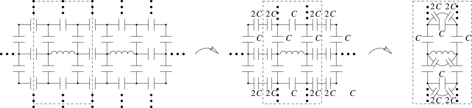
Figure 8: Low-frequency renormalisation scheme for the transformation of an infinite line of alternating coils and capacitors in a 2D capacitor lattice with bonds of capacity $C$ (left graph) to an infinite ladder of capacitors with only one horizontal capacitor replaced by a coil (right graph). (In the second and third graph, a bond with two capacitors in series always represents two times $2C$ in series.)

The systems studied in the preceding sections could be reduced to effective 1D problems, because (i) the arrays covered the whole width of the electrodes and (ii) periodic boundary conditions were assumed in $y$-direction. In this section, by contrast, we will examine simple regular 1D arrays in an infinite square lattice. The observed changes turn out to be considerable, and sometimes not only shift the frequencies, but qualitatively change the spectrum.

The first example we want to inspect consists in a single line of alternating inductors and capacitors embedded in an otherwise pure capacitor lattice, as shown in the leftmost graph of Fig. 8. Alternatively, this line is generated by replicating the unit cell of Fig. 5(c) only in $x$-direction.

Figure 9: Eigenfrequencies $\omega$ in units of $\omega_{0}$ for a line of $N$ alternating coils and capacitors embedded in an infinite capacitor lattice. The circles represent numerically calculated eigenfrequencies, obtained with the spectral method. The dashed lines are the analytical large $N$ asymptotes, $\tilde{\omega}_{\rm LF}\simeq 1/\sqrt{2\sqrt{2}-1}\simeq 0.7395$ and $\tilde{\omega}_{\rm HF}\simeq 1/\sqrt{\sqrt{3}-1}\simeq 1.1688$ discussed in the text.

Its eigenfrequencies are obtained very accurately with the so-called spectral method, initially proposed by Straley Straley , Bergman Bergman and Milton Milton , and later adapted to 2D lattices by Clerc, Giraud, Luck and co-workers Clerc1996 ; Luck1998 , employing a Green’s function formalism developped by McCrea and Whipple McCrea in the context of random walks; (see also Spitzer Spitzer ). This approach connects the impedance resonances of a (not necessarily ordered) cluster to the eigenvalues of a non-symmetric square matrix, which — in general — have to be evaluated numerically. The latter version of the spectral method assumes the cluster to be located in the middle of an infinite lattice — just as in the examples we wish to study. To obtain similar results from an ENR calculation one would have to incorporate the cluster in a much larger capacitor network (compared to the cluster’s size) — a situation which is computationally very demanding.

The eigenfrequencies of the line of alternating coils and capacitors, obtained via the spectral method, are plotted with dots in Fig. 9 as a function of the number of coils, $N$. In the limit of large $N$, the lowest eigenmode shows the full translational invariance of the system, and thus has the same current distribution in every vertical stripe. This implies that the left and right boundary of the stripe can be thought of as attached together. In order to perform this operation, illustrated in Fig. 8, one has to (i) chose a stripe which is symmetric about one of the coils, (ii) replace all horizontal capacitors of capacity $C$ in all pure capacitor columns by two capacitors in series, with capacity $2C$ each, (iii) cut between the doubled capacitors, and (iv) tie the corresponding vacant ends of the stripe together. One ends up with an infinite ladder with horizontal steps of $2C$ (two times $2C$ in series, the whole parallel to a capacitor $C$), except for one step which contains a coil instead of the single capacitor; the vertical legs of the ladder consist of capacitors $C$ (cf. rightmost graph in Fig. 8). The capacities may then be summed up in a procedure analogous to eqs. (13) and (14), yielding a total capacity of $C(2\sqrt{2}-1)$, and thus the low-frequency asymptote $\tilde{\omega}_{\rm LF}\simeq 1/\sqrt{2\sqrt{2}-1}\simeq 0.7395$ (lower dashed line in Fig. 9).

The position of the high-frequency asymptote $\tilde{\omega}_{\rm HF}\simeq 1/\sqrt{\sqrt{3}-1}\simeq 1.1688$ (upper dashed line in Fig. 9), on the opposite side of the spectrum, can be calculated almost analogously: in the limit of an infinite $LC$ chain in its highest eigenmode, the currents through two neighbouring coils are at any moment antiparallel, but of the same magnitude. The capacitors separating the coils horizontally are thus located at current nodes and can be omitted. The corresponding ladder looks the same as the one shown in the right of Fig. 8, except for the fact that all capacitors of $2C$ (on the bent lines) have to be removed.

Comparison to the case with periodic boundaries in $y$ direction, studied in Sec. 2 (eq. (12) in particular), shows that the shift of a resonance depends on its location in the spectrum: at the low-frequency edge, formerly located at $\tilde{\omega}\simeq\sqrt{5/3}\simeq 1.291$, now at $\tilde{\omega}\simeq 0.7395$, the renormalisation is stronger than at the high-frequency boundary (formerly $\tilde{\omega}\simeq\sqrt{2}\simeq 1.414$, now $\tilde{\omega}\simeq 1.1688$). The reason for this behaviour lies in the different renormalisation schemes which — as pointed out above — couple the inductors to an equivalent capacity which is less enhanced for high frequencies than for low ones.

The second cluster we are going to study in this section is a straight line of $N$ coils in series embedded in a pure capacitor environment.

Figure 10: Eigenfrequencies $\omega$ in units of $\omega_{0}$ for a continuous line of $N$ coils embedded in an infinite capacitor lattice. The circles represent numerically calculated eigenfrequencies, obtained with the spectral method. The dashed lines are the large $N$ asymptotes, $\tilde{\omega}_{\rm LF}\simeq\sqrt{1.16/N}$ and $\tilde{\omega}_{\rm HF}\simeq\sqrt{1+\sqrt{2}}\simeq 1.5538$ (see text).

The resonance frequencies of this “lattice worm”, obtained via the spectral method, are plotted with dots in Fig. 10. For large $N$ and at high frequencies, the cluster can again be reduced to almost independent stripes.

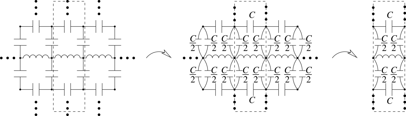
Figure 11: High-frequency renormalisation scheme for an infinite line of coils in a 2D capacitor lattice (left graph), ending up in an infinite capacitor ladder with only one coil (right graph).

The corresponding renormalisation scheme is illustrated in Fig. 11, and ends up in an infinite ladder with legs of capacity $C/2$ and steps of capacity $C$ (except for the central step which is a coil of inductance $L$). Summing up each semi-infinite capacitor ladder yields $C_{\rm inf}=\frac{1}{2}C(1+\sqrt{2})$ (cf. eqs (13) and (14)), and thus the high-frequency asymptote $\tilde{\omega}_{\rm HF}\simeq\sqrt{1+\sqrt{2}}\simeq 1.5538$ (upper dashed line in Fig. 10). Comparison to the periodic case, eq. (9), where $\tilde{\omega}\to\sqrt{3}$ for $m=N$ and $N\to\infty$, shows that the renormalisation shifts are rather modest at high frequencies.

At low frequencies, by contrast, the infinite environment has drastic effects: as can be seen from Fig. 10, the lowest resonance tends to zero frequency as the length of the worm increases. The corresponding density of states therefore shows no gap at low frequencies — as opposed to the density of states (10) of the periodic system, illustrated in the last graph of Fig. 3.

The reason for this behaviour can be qualitatively understood in a simple picture representing the whole worm of $N$ coils as a dipole of total inductance $NL$. This dipole is thought to be coupled to a single capacitor bearing the entire capacity of the lattice. In this model, the lowest resonance would thus be found at $\omega\simeq\sqrt{1/(NLC_{\rm lat})}$. As pointed out in Appendix A, the dipole model evaluates the entire lattice capacity to roughly $C_{\rm lat}\simeq C$, a value which allows to reproduce the exact resonance frequency $\tilde{\omega}=1$ for a single coil ($N=1$) in a 2D capacitor lattice. For increasing $N$, $C_{\rm lat}$ is found slightly reduced since more and more capacitors are replaced by coils. In the limit of large $N$, the numerically calculated groundstate fits very accurately to $\tilde{\omega}\simeq\sqrt{1.16/N}$ (lower dashed line in Fig. 10).

In the same manner, the dipole model predicts a resonance frequency of $\tilde{\omega}_{m}\propto\sqrt{m/N}$ for the $m$.th mode, with a proportionality constant of the order of unity, since the current nodes split the “worm” into $m$ almost independent segments of $N/m$ coils each. Comparison to the numerically evaluated eigenfrequencies shows that this scenario works well for $m\lesssim 5$, but turns out to be too simplistic for the higher excited modes.

On more general grounds, and observing that second-order terms do not improve the reproduction of the data, one may try an ansatz of the form

$$\tilde{\omega}_{m}\;\simeq\;\sqrt{\frac{\alpha_{m}}{N}}\;+\;\sqrt{\frac{\beta_{m}}{N}}^{3}\;\text{.}$$ (34)

A linear dependence of the parameters, $\alpha_{m}=-0.40+1.57m$ and $\beta_{m}=-0.56+0.98m$, deduced by a fit for $N=200\ldots 1000$ and $m=1\ldots 30$, reproduces the numerically calculated resonance frequencies very accurately for a wide range of $N$ and $m$, as long as $N/m$ is large ($\gtrsim 5$).

We also note that the fitted $\alpha$, with a slope of $1.57$, concords with an analytical result obtained by Clerc et al. Clerc1996 , stating that $\tilde{\omega}_{m}\sim\sqrt{\frac{\pi}{2}m/N}$ for the bulk states of a long linear cluster, i.e. if both $m$ and $N$ are large.

5 Conclusions and outlook

In this article, we have studied the dielectric resonance spectra of ordered passive arrays, typically — although not necessarily — constituted of inductive and capacitive elements. Similar arrays, based on split-ring resonators, have recently been used to assemble metamaterials for the microwave regime, exhibiting negative refraction and other exotic properties Pendry2004 ; Seddon2003 ; Grbic2004 .

In the first part, we have calculated the resonance frequencies of several arrays by solving a system of differential equations deduced directly from Kirchhoff’s rules — a technique which allows for a straightforward interpretation of the spectra and thus provides a good handle for the influence of each of the array’s parameters. On the other hand, each new circuit requires a separate individual analysis, relying on the solution of increasingly complicated recurrence relations as the unit cell of the array gets richer in structure.

An alternative approach, presented in Sec. 3, deduces the resonance frequencies from the array’s transfer matrix, i.e. a matrix connecting the state vectors (a combination of currents and voltages at each vertex) at both ends of the cluster to each other. Within this formalism, the array is shown to be in resonance if all eigenvalues of its transfer matrix are unity for a given frequency — a condition which is demonstrated to be equivalent to the more familiar definition of a divergent impedance for a cluster between two electrodes, namely vanishing net current through the sample at finite applied voltage. Even large arrays, with complex unit cells, can be easily analysed with this algorithm since, in a handier reformulation, the new resonance condition, eq. (25), does not require the computation of the transfer matrix of the whole array, but only of a single unit cell. The latter is most conveniently evaluated by multiplication of the transfer matrices of a few standard situations — two in our case, cf. eq. (17a), where the 2D arrays reduce to two-legged ladders due to the assumption of periodic boundary conditions along the electrodes — a task which can be performed using symbolic computation software. In its final form, the resonance frequencies are typically given as the roots of a polynomial whose degree depends on the complexity of the unit cell.

If, however, the cluster happens to be embedded in a much larger lattice, periodic boundary conditions are not a pertinent approximation, and the resonance frequencies are generically not available in closed form anymore. In this case, major changes in the spectrum have to be expected, of which some can be understood in terms of renormalisation, while others cannot. Among the latter, one may recall the example of a longer growing linear array: embedded in a periodic medium, the spectrum remains gapped for any length of the cluster; if, by contrast, the same cluster is isolated in a homogeneous network, the gap closes with increasing length and the resonance spectrum carries the signature of one or more rather independent two-dimensional dipoles.

The tools discussed in this article may be useful for the design of circuits with a custom electric response. Such devices could be used for labelling — just as bar codes — which could be read by an automated system.

For the future it would be undoubtedly desirable, especially in the perspective of the already mentioned development of metamaterials with negative refraction, to take into account the magnetic part of the optical response, with the aim to create devices having both, tunable dielectric and magnetic resonances.

Appendix A Dipole approximation for linear clusters

The scenario presented in the following is based on the idea that the current flowing through a linear cluster isolated in a capacitor lattice flows back through the lattice with a current distribution which, in the lowest eigenmode, resembles the field lines of a dipole in 2D electrostatics (see Fig. 12).

Figure 12: Current distribution (dashed lines) of a linear cluster of length $N=1$ in the dipole approximation. (The lower half-plane has been omitted for clarity.)

This idea is supported by the spectral method, in the framework of which the electric potential $V_{\mathbf{r}}$ induced by a single horizontal coil, located at the origin, is known to be given by Clerc1996

$$\lambda V_{\mathbf{r}}\;=\;-W\,\left[G_{\mathbf{r}+\frac{1}{2}\mathbf{\hat{x}}}-G_{\mathbf{r}-\frac{1}{2}\mathbf{\hat{x}}}\right]\;\text{,}$$ (35)

where $\lambda$ is a frequency-dependent proportionality constant, $W$ the voltage measured between the ends of the coil, and $G_{\mathbf{r}}$ the 2D lattice Green’s function. Far from the coil, for $\left|\mathbf{r}\right|\gg 1$, the lattice Green’s function may be replaced by its continuous counterpart, $G_{\mathbf{r}}\simeq-\frac{1}{2\pi}\ln\left|\mathbf{r}\right|$, and eq. (35) reduces to a 2D dipole potential

$$\lambda V_{\mathbf{r}}\;\simeq\;-W\frac{\partial}{\partial x}G_{\mathbf{r}}\;\simeq\;\frac{W}{2\pi}\;\frac{x}{x^{2}+y^{2}}\;\equiv\;\frac{W}{2\pi}\;\frac{\cos\varphi}{\left|\mathbf{r}\right|}\;\text{.}$$ (36)

In this approximation, the current distribution follows the field lines

$$r(\varphi)\;=\;\frac{l}{\pi}{\sin{\varphi}}$$ (37)

where $l$ is the length of the field line (in units of the lattice spacing). In order to calculate the resonance frequency of a cluster embedded in an infinite capacitor lattice, one has to assign an equivalent capacity, $C_{\rm lat}$, to the entire lattice. Of course, $C_{\rm lat}$ depends on the current distribution: in general, capacitors almost perpendicular to the current lines contribute only little to $C_{\rm lat}$, while capacitors following the current lines contribute as if they were in series. At great distance from the cluster, the lattice behaves as if it were assembled by independent lines of capacitors, hence all in parallel, contributing each as the inverse of its length:

$$C_{\rm lat}\;\simeq\;\sum\limits_{k}\frac{C}{l_{k}}$$ (38)

The sum in eq. (38) runs over all possible current paths, and — in order to avoid divergences — the counting has to be done very carefully. In our example of a single coil in an infinite lattice, this may be achieved by supposing that the current can only leave the $x$-axis at spots where a vertical capacitor is present. Following the illustration of Fig. 12, this amounts to retaining only current lines passing through $(x=k+\frac{1}{2},y=1)$ with $k=0,1,2,\ldots$. In coordinates of the field lines (37), these points are described by

$$l_{k} = \pi\left[1+\left(k+{\textstyle\frac{1}{2}}\right)^{2}\right]$$ (39a)

$$\sin\varphi_{k} = \frac{1}{\sqrt{1+\left(k+\frac{1}{2}\right)^{2}}}\;\text{.}$$ (39b)

The first equation can be used to select only the desired current lines, as shown in Fig. 12. Pinning the field lines in this way has a twofold virtue, namely on the short side to set a lower boundary for the path length $l_{k}$ in (38), and to avoid the logarithmic divergence on the long side, $l_{k}\to\infty$. After substitution in (38), and taking into account contributions from the lower half-plane, we obtain

$$C_{\rm lat} \simeq \frac{2C}{\pi}\sum\limits_{k=0}^{\infty}\frac{1}{1+(k+\frac{1}{2})^{2}}$$ (40)

$$\simeq \frac{2C}{\pi}\int\limits_{0}^{\infty}\frac{{\rm d}k}{1+k^{2}}\;=\;C\;\text{.}$$

(The sum in the first line may be thought of as a midpoint trapeze approximation for the integral in the second line).

According to the dipole approximation, an isolated coil in a 2D capacitor network thus resonates at $\omega=1/\sqrt{LC_{\rm lat}}\simeq 1/\sqrt{LC}\equiv\omega_{0}$ — which is the exact result known from the spectral method.

References

- (1) J.B. Pendry and D.R. Smith, Physics Today, June Issue (2004), 37.
- (2) V.G. Veselago, Sov. Phys. Usp. 10, (1968), 509.
- (3) N. Seddon and T. Bearpark, Science 302, (2003) 1537.
- (4) A. Grbic and G.V. Eleftheriades, Phys. Rev. Lett. 92, (2004) 117403.
- (5) L. Raymond, J.-M. Laugier, S. Schäfer, and G. Albinet, Eur. Phys. J. B 31 (2003), 355.
- (6) A.P. Vinogradof and A.K. Sarychev , Sov. Phys. JETP 58 (1983), 665.
- (7) A.K. Sarychev, D.J. Bergman and Y.M. Strelniker, Phys.Rev. B 48 (1993), 3145.
- (8) L. Tortet, J.R. Gavarri, J. Musso, G. Nihoul, J.P. Clerc, A.N. Lagarkov and A. K. Sarychev, Phys. Rev. B 58 (1998).
- (9) J.P. Straley, J. Phys. C 12 (1979), 2143.
- (10) D.J. Bergman, Phys. Rep. 43 (1978), 377; Phys. Rev. Lett. 44 (1980), 1285; Phys. Rev. B 23 (1981), 3058; Ann. Phys. 138 (1981), 78.
- (11) G.W. Milton, Appl. Phys. Lett. 37 (1980), 300; J. Appl. Phys. 52, (1981), 5286, 5294; Phys. Rev. Lett. 46 (1981), 542.
- (12) J.P. Clerc, G. Giraud, J.M. Luck and Th. Robin, J. Phys. A 29 (1996), 4781.
- (13) Th. Jonckheere and J.M. Luck, J. Phys. A 31 (1998), 3687.
- (14) G. Albinet and L. Raymond, Eur. Phys. J. B 13 (2000), 561.
- (15) W.H. McCrea and F.J. Whipple, Proc. Royal Soc. Edinburgh 60 (1940), 281.
- (16) F. Spitzer, Principles of Random Walk, Van Nostram inc., Princeton, (1964).