Shape complexity and fractality of fracture surfaces of swelled isotactic polypropylene with supercritical carbon dioxide

Abstract

We have investigated the fractal characteristics and shape complexity of the fracture surfaces of swelled isotactic polypropylene Y1600 in supercritical carbon dioxide fluid through the consideration of the statistics of the islands in binary SEM images. The distributions of area $A$, perimeter $L$, and shape complexity $C$ follow power laws $p(A)\sim A^{-(\mu_{A}+1)}$, $p(L)\sim L^{-(\mu_{L}+1)}$, and $p(C)\sim C^{-(\nu+1)}$, with the scaling ranges spanning over two decades. The perimeter and shape complexity scale respectively as $L\sim A^{D/2}$ and $C\sim A^{q}$ in two scaling regions delimited by $A\approx 10^{3}$. The fractal dimension and shape complexity increase when the temperature decreases. In addition, the relationships among different power-law scaling exponents $\mu_{A}$, $\mu_{B}$, $\nu$, $D$, and $q$ have been derived analytically, assuming that $A$, $L$, and $C$ follow power-law distributions.

I Introduction

Polypropylene, being one of the fastest growing engineering plastics, has wide industrial and everyday life applications due to its intrinsic properties such as low density, high melting point, high tensile strength, rigidity, stress crack resistance, abrasion resistance, low creep and a surface which is highly resistance to chemical attack, and so on Moore (1996). Impregnation of nucleating agents allows the polymer to be crystallized at a higher temperature during processing and changes a lot the mechanical and optical performance of the resultant polymer matrix Xu et al. (2003); Iroh and Berry (1996). In such nucleating agent impregnating processes, supercritical fluids are well-established swelling solvents whose strength can be tuned continuously from gas-like to liquid-like by manipulating the temperature and pressure. Especially, supercritical carbon dioxide is a good swelling agent for most polymers and will dissolve many small molecules Chiou et al. (1985); Kamiya et al. (1988); Berens et al. (1992); Kamiya et al. (1998), except for some fluoropolymers and silicones Tuminello et al. (1995). This provides the ability to control the degree of swelling in a polymer Fleming and Koros (1986); Pope and Koros (1996); Condo et al. (1996) as well as the partitioning of small molecule penetrants between a swollen polymer phase and the fluid phase Vincent et al. (1997); Kazarian et al. (1998).

The morphology of fracture surfaces of a material is of great concerns and interests in many studies Cherepanov et al. (1995); Fineberg and Marder (1999). A frequently used tools is fractal geometry pioneered by Mandelbrot’s celebrated work Mandelbrot (1983). Specifically, fractal geometry has been widely applied to the topographical description of fracture surfaces of metals Mandelbrot et al. (1984); Wendt et al. (2002), ceramics Mecholsky et al. (1989); Thompson et al. (1995); Celli et al. (2003), polymers Chen and Runt (1989); Yu et al. (2002), concretes Dougan and Addison (2001); Wang and Diamond (2001); Issa et al. (2003); Yan et al. (2003), alloys Shek et al. (1998); Wang et al. (1999); Betekhtin et al. (2002); Eftekhari (2003), rocks Xie et al. (2001); Babadagli and Develi (2003); Zhou and Xie (2003), and many others. There are many different approaches adopted in the determination of fractal dimensions of fracture surfaces and the estimated fractal dimensions from different materials vary from case to case and are not universal Wang (2004).

Concerning the fractal characterization of the fracture surfaces of polypropylene, it was found that the fractal dimension of the fracture surfaces is less than 2.12 Yu et al. (2002). In this paper, we investigate the shape complexity and fractality of fracture surfaces of nucleating agents impregnated isotactic polypropylene (Y1600) swelled with supercritical carbon dioxide based on the area-perimeter relationship Mandelbrot (1983); Lovejoy (1982); Mandelbrot et al. (1984). We shall see that the fractal dimension of the fracture surface of supercritical dioxide swelled polypropylene is much higher than that without swelling and decreases with increasing temperature.

II Experimental

The isotactic polypropylene (Y1600) powder we have used has an average diameter of $3\sim 4~{}mm$. Fifteen grams of isotactic polypropylene powder was melt in an oven at $200\,^{\circ}\mathrm{C}$ and then made into film with a thickness of 0.3 $mm$ by using a press machine with a pressure of 0.5 GN. The size of the standard film samples was $1mm\times 3mm$ and are refluxed with acetone for twenty four hours to remove the impurities, and then annealed at $200\,^{\circ}\mathrm{C}$ for two hours. The nucleating agent we used was NA21.

The schematic flow chart of the experimental apparatus is illustrated in Fig. 1. The experimental apparatus consists mainly of a gas cylinder, a gas booster, a digital pressure gauge, an electrical heating bath, and valves and fittings of different kinds. The system was cleaned thoroughly using suitable solvents and dried under vacuum. Isotactic PP films marked from one to twelve were placed in the high pressure cell together with desired amount ($1\%$ wt) of nucleating agent (NA21). The system was purged with $\rm{CO}_{2}$ and after the system had reached the desired temperature and thermal equilibrium, $\rm{CO}_{2}$ was charged until the desired pressure was reached. The impregnation process lasted for four hours and then depressurized the $\rm{CO}_{2}$ from the high pressure cell rapidly. Then the vessel was cooled and opened, and the specimens were taken out for analysis. All of the metallic parts in contact with the studied chemicals were made of stainless steel. The apparatus was tested up to 35 MPa. The total volume of the system is 500 mL.

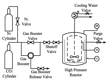
Figure 1: Schematic flow chart of the experimental apparatus.

The experiments were performed at fixed pressure of 7.584 MPa and at four different temperatures of $T=60\,^{\circ}\mathrm{C}$, $80\,^{\circ}\mathrm{C}$, $100\,^{\circ}\mathrm{C}$, and $120\,^{\circ}\mathrm{C}$. For each sample, we took ten SEM pictures at magnification of 5000 or 10000. The pictures have 256 grey levels. Due to the nature of area-perimeter approach, the results are irrelevant to the magnification Mandelbrot (1983). A grey-level picture was transformed into black-and-white image for a given level set $\epsilon$ according to the criterion that a pixel is black if its grey level is larger than $256\epsilon$ and is white otherwise. The resultant binary image has many black islands. A typical binary image of islands is shown in Fig. 2. In our calculations, we have used eleven level sets from 0.45 to 0.95 spaced by 0.05 for each SEM picture.

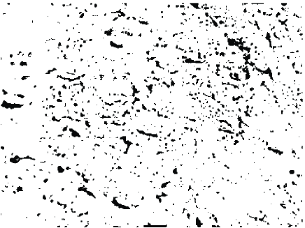
Figure 2: Image of the recognized islands from a typical SEM picture of swelled isotactic polypropylene impregnated with NA21 at level set of 0.7.

III Fractality and shape complexity

III.1 Rank-ordering statistics of area and perimeter

In order to estimate the probability distribution of a physical variable empirically, several approaches are available. For a possible power-law distribution with fat tails, cumulative distribution or log-binning technique are usually adopted. A similar concept to the complementary distribution, called rank-ordering statistics Sornette (2000), has the advantage of easy implementation, without loss of information, and less noisy.

Consider $n$ observations of variable $x$ sampled from a distribution whose probability density is $p(x)$. Then the complementary distribution is $P(y>x)=\int_{x}^{\infty}p(y)dy$. We sort the $n$ observations in non-increasing order such that $x_{1}\geq x_{2}\geq\cdots\geq x_{R}\geq\cdots\geq x_{n}$, where $R$ is the rank of the observation. It follows that $nP(x\geq x_{R})$ is the expected number of observations larger than or equal to $x_{R}$, that is,

$$nP(x\geq x_{R})=R~{}.$$ (1)

If the probability density of variable $x$ follows a power law that $p(x)\sim x^{-(1+\mu)}$, then the complementary distribution $P(x)\sim x^{-\mu}$. An intuitive relation between $x_{R}$ and $R$ follows

$$x_{R}\sim R^{-1/\mu}~{}.$$ (2)

A rigorous expression of (2) by calculating the most probable value of $x_{R}$ from the probability that the $R$-th value equals to $x_{R}$ gives Sornette (2000)

$$x_{R}\sim\left(\frac{\mu n+1}{\mu R+1}\right)^{1/\mu}~{}.$$ (3)

when $\mu R\gg 1$ or equivalently $1\ll R\leq N$, we retrieve (2). A plot of $\ln x_{R}$ as a function of $\ln R$ gives a straight line with slope $-1/\mu$ with deviations for the first a few ranks if $x$ is distributed according to a power law of exponent $\mu$.

We note that the rank-ordering statistics is nothing but a simple generalization of Zipf’s law Zipf (1949); Mandelbrot (1983); Sornette (2000) and has wide applications, such as in linguistics Mandelbrot (1954), the distribution of large earthquakes Sornette et al. (1996), time-occurrences of extreme floods Mazzarella and Rapetti (2004), to list a few. More generally, rank-ordering statistics can be applied to probability distributions other than power laws, such as exponential or stretched exponential distributions Laherrere and Sornette (1998), normal or log-normal distributions Sornette (2000), and so on.

Figure 3 illustrates the log-log plots of the rank-ordered areas $A$ at different temperatures. There is clear power-law dependence between $A$ and its rank $R$ with the scaling ranges spanning over about two decades. Least-squared linear fitting gives $1/\mu_{A}=0.80\pm 0.05$, $1/\mu_{A}=0.63\pm 0.02$, $1/\mu_{A}=0.61\pm 0.03$, and $1/\mu_{A}=0.85\pm 0.04$ with decreasing temperatures, where the errors are estimated by the r.m.s. of the fit residuals. Using $\sigma_{\mu_{A}}=\sigma_{1/\mu_{A}}/\mu_{A}^{2}$, we obtain the power-law exponents $\mu_{A}=1.24\pm 0.08$, $\mu_{A}=1.59\pm 0.06$, $\mu_{A}=1.64\pm 0.09$, and $\mu_{A}=1.18\pm 0.05$ with decreasing temperatures.

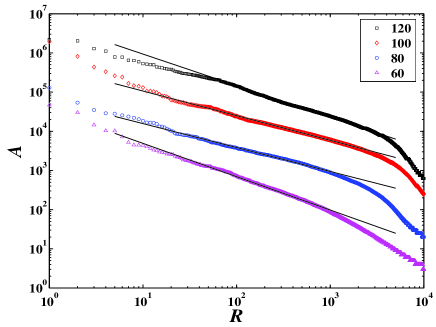
Figure 3: Log-log plot of the rank-ordered areas $A$ at different temperatures shown in the legend. The plots are translated vertically for clarity. The solid lines are linear fits to the data at $59\leq R\leq 3890$ for $T=120\,^{\circ}\mathrm{C}$, $10\leq R\leq 1995$ for $T=100\,^{\circ}\mathrm{C}$, $22\leq R\leq 1000$ for $T=80\,^{\circ}\mathrm{C}$, and $8\leq R\leq 800$ for $T=60\,^{\circ}\mathrm{C}$, respectively.

Figure 4 shows the log-log plots of the rank-ordered perimeters $L$ at different temperatures. There are also clear power-law relations between $L$ and its rank $R$ whose scaling ranges spanning over about three decades. Least-squared linear fitting gives $1/\mu_{L}=0.56\pm 0.02$, $1/\mu_{L}=0.51\pm 0.01$, $1/\mu_{L}=0.55\pm 0.03$, and $1/\mu_{L}=0.71\pm 0.03$ with decreasing temperatures. We thus obtain the power-law exponents $\mu_{L}=1.78\pm 0.07$, $\mu_{L}=1.95\pm 0.05$, $\mu_{L}=1.83\pm 0.12$, and $\mu_{L}=1.41\pm 0.06$ with decreasing temperatures. It is noteworthy that the scaling ranges of the rank-ordering of both $A$ and $P$ are well above two decades broader than most of other experiments with scaling ranges centered around 1.3 orders of magnitude and spanning mainly between 0.5 and 2.0 Malcai et al. (1997); Avnir et al. (1998).

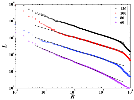
Figure 4: Log-log plot of the rank-ordered perimeters $L$ at different temperatures marked in the legend. The plots are translated vertically for clarity. The solid lines are linear fits to the data at $5\leq R\leq 3890$ for $T=120\,^{\circ}\mathrm{C}$, $24\leq R\leq 3000$ for $T=100\,^{\circ}\mathrm{C}$, $16\leq R\leq 2000$ for $T=80\,^{\circ}\mathrm{C}$, and $10\leq R\leq 1500$ for $T=60\,^{\circ}\mathrm{C}$, respectively.

III.2 Scaling between area and perimeter

If an island is fractal, its area $A$ and perimeter $L$ follow a simple relation,

$$L^{1/D}\sim A^{1/2}~{},$$ (4)

where $D$ is the fractal dimension describing the wiggliness of the of the perimeter. For $D=1$, the perimeter of the island is smooth. For $D=2$, the perimeter becomes more and more contorted to fill the plane. This area-perimeter relation (4) can also be applied to many islands when they are self-similar in the sense that the ratio of $L^{1/D}$ over $A^{1/2}$ is constant for different islands Mandelbrot (1983). It has been used to investigate the geometry of satellite- and radar-determined cloud and rain regions by drawing $A$ against $L$ for different regions in a log-log plot Lovejoy (1982). The slope of the straight line obtained by performing a linear regression of the data gives $2/D$.

Following the same procedure, we plotted for each temperature $L$ against $A$ for all islands identified at different level sets. The resultant scatter plot for a given temperature shows nice collapse to a straight line. The four slopes are $D=1.34\pm 0.08$ for $T=60\,^{\circ}\mathrm{C}$, $D=1.32\pm 0.07$ for $T=80\,^{\circ}\mathrm{C}$, $D=1.31\pm 0.08$ for $T=100\,^{\circ}\mathrm{C}$, and $D=1.28\pm 0.09$ for $T=120\,^{\circ}\mathrm{C}$, respectively. The errors were estimated by the r.m.s. of the fit residuals.

However, a closer investigation of the scatter plots shows that there are two scaling regions with a kink at around $A=1000$. To have a better view angle, we adopt an averaging technique for both $A$ and $L$. We insert $n-2$ points in the interval $[\min(A),\max(A)]$ resulting in $\min(A)=a_{0}<a_{1}<a_{2}<\cdots<a_{n}=\max(A)$ so that $a_{i}$’s are logarithmically spaced. We can identify all islands whose areas fall in the interval $[a_{i},a_{i+1})$. The geometric means of $L$ and $A$ are calculated for these islands, denoted as $\langle{L}\rangle$ and $\langle{A}\rangle$. The calculated means $\langle{L}\rangle$ and $\langle{A}\rangle$ are plotted in Fig. 5. The two scaling regions are fitted respectively with two straight lines and we have $D_{1}=1.42\pm 0.06$ for $T=60\,^{\circ}\mathrm{C}$, $D_{1}=1.33\pm 0.06$ for $T=80\,^{\circ}\mathrm{C}$, $D_{1}=1.33\pm 0.07$ for $T=100\,^{\circ}\mathrm{C}$, and $D_{1}=1.30\pm 0.05$ for $T=120\,^{\circ}\mathrm{C}$, in the first region that $\langle{A}\rangle<1000$ and $D_{2}=1.96\pm 0.07$ for $T=60\,^{\circ}\mathrm{C}$, $D_{2}=1.89\pm 0.24$ for $T=80\,^{\circ}\mathrm{C}$, $D_{2}=2.15\pm 0.11$ for $T=100\,^{\circ}\mathrm{C}$, and $D_{2}=2.07\pm 0.14$ for $T=120\,^{\circ}\mathrm{C}$ in the second region that $\langle{A}\rangle>1000$.

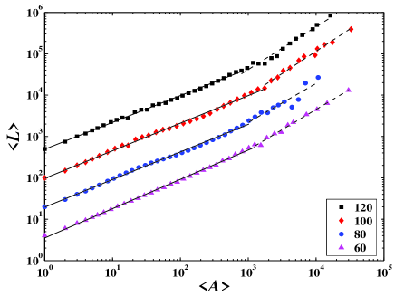
Figure 5: Plots of $\langle{L}\rangle$ with respect to $\langle{A}\rangle$ at different temperatures. The plots are translated vertically for clarity. We note that $\langle{L}\rangle=4$ when $\langle{A}\rangle=1$ in all the four plots.

It is very interesting to notice that $L\propto A$ for large areas. Under the consumption that the islands are fractals, this relation can be interpreted that the perimeters of the large islands are so wiggly that they can fill the plane. However, there are simple models that can deny this consumption of self-similarity. Consider that we have a set of strip-like islands with length $l$ and width $w$. We have $L=2(l+w)$ and $A=lw$. When $w$ is fixed and $l\gg w$, it follows that $L\propto A$. This simple model can indeed explain the current situation. For cracked polypropylene, there are big strip-like ridges in the intersection whose surface is relatively smooth. For small islands, the fractal nature is more sound.

According to the additive rule of codimensions of two intersecting independent sets, the fractal dimension of the surface is $D_{s}=D_{1}+1$ Mandelbrot (1983). Therefore, $D_{s}=2.42\pm 0.06$ for $T=60\,^{\circ}\mathrm{C}$, $D_{s}=2.33\pm 0.06$ for $T=80\,^{\circ}\mathrm{C}$, $D_{s}=2.33\pm 0.07$ for $T=100\,^{\circ}\mathrm{C}$, and $D_{s}=2.30\pm 0.05$ for $T=120\,^{\circ}\mathrm{C}$. We see that the fractal dimension $D_{s}$ increases with decreasing temperature. In other words, with the increase of temperature, the surface becomes smoother.

Assuming that $p(A)\sim A^{-(\mu_{A}+1)}$ and $p(L)\sim L^{-(\mu_{L}+1)}$, we can estimate the fractal dimension $D$ in (4) according to the relation $p(A)dA=p(L)dL$ such that

$$D=2\mu_{A}/\mu_{L}~{}.$$ (5)

The four estimated values of $D$ using this relation (5) are 1.67, 1.79, 1.63, and 1.40 with increasing temperature. The discrepancy from $D_{1}$ is remarkable ($15\%$, $25\%$, $18\%$, and $7\%$, accordingly). The source of this discrepancy is threefold. Firstly, the power-law distributions of $A$ and $L$ have cutoffs at both ends of small and large values so that the derivation of (5) is not rigorous. Secondly, the determination of the scaling ranges may cause errors. Thirdly, the scaling ranges of the three power laws are not consistent with each other.

III.3 Shape complexity

To quantify the shape complexity of an irregular fractal object, besides the fractal dimension, there are other relevant measures related to the fractal nature Catrakis and Dimotakis (1998); Kondev et al. (2000). For a $d$-dimensional hypersphere, its surface and volume are related by

$$S_{d,sph}=\frac{1}{k_{d}}V_{d,sph}^{(d-1)/d}~{},$$ (6)

where

$$k_{d}=\frac{\Gamma^{1/2}(1+d/2)}{d\pi^{1/2}}~{}.$$ (7)

Since a hypersphere has the maximal enclosed volume among the objects with a given surface $S_{d}$, we have

$$S_{d}\geq\frac{1}{k_{d}}V_{d}^{(d-1)/d}~{}.$$ (8)

Then the following dimensionless ratio

$$C_{d}\triangleq\frac{k_{d}S_{d}}{V_{d}^{(d-1)/d}}$$ (9)

describes the irregularity or complexity of the investigated object Catrakis and Dimotakis (1998). It follows that $1\leq C_{d}\leq\infty$. The limits are reached at $C_{d}=1$ for hyperspheres and $C_{d}=\infty$ for fractals. For real fractal objects, sometimes known as prefractals Addison (2000), the scaling range is not infinite. The shape complexity $C_{d}$ is thus finite. In the case of $d=2$, we have

$$1\leq C\triangleq\frac{L}{2\pi^{1/2}A^{1/2}}\leq\infty~{}.$$ (10)

This dimensionless measure of shape complexity has been applied to scalar field of concentration in turbulent jet at high Reynolds numbers Catrakis and Dimotakis (1998); Catrakis et al. (2002).

In Fig. 6 is shown the log-log plot of the rank-ordered shape complexity $C$ at different temperatures. The power-law dependence $C\sim R^{-1/\nu}$ implies a power-law probability density of shape complexity, that is,

$$p(C)\sim C^{-(\nu+1)}~{}.$$ (11)

We find that $\nu=3.97\pm 0.11$ for $T=60\,^{\circ}\mathrm{C}$, $\nu=4.61\pm 0.17$ for $T=80\,^{\circ}\mathrm{C}$, $\nu=4.93\pm 0.20$ for $T=100\,^{\circ}\mathrm{C}$, and $\nu=5.22\pm 0.17$ for $T=120\,^{\circ}\mathrm{C}$. The mean logarithmic complexity $\langle\ln C\rangle=1/(\nu-1)$ Catrakis and Dimotakis (1998) is calculated to be 0.34, 0.28, 0.25, and 0.24 with increasing temperature. In other words, the shape complexity of the islands decreases with increasing temperature. This is consistent with the fact the $D$ decreases with increasing temperature.

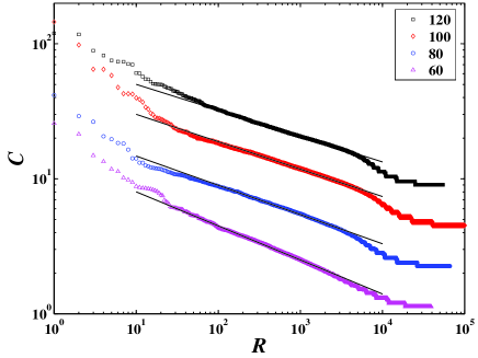
Figure 6: Log-log plot of the rank-ordered shape complexity $C$ at different temperatures. The plots are translated vertically for clarity. The solid lines are linear fits to the data at $40\leq R\leq 3890$ for $T=120\,^{\circ}\mathrm{C}$, $24\leq R\leq 5000$ for $T=100\,^{\circ}\mathrm{C}$, $40\leq R\leq 3000$ for $T=80\,^{\circ}\mathrm{C}$, and $25\leq R\leq 1500$ for $T=60\,^{\circ}\mathrm{C}$, respectively.

Following the procedure in Sec. III.2, we calculate the means, $\langle{A}\rangle$ and $\langle{C}\rangle$. The results are shown in Fig. 7. Again, we see two scaling regions guided by straight lines fitted to the data

$$C\sim A^{q}~{}.$$ (12)

The slopes are respectively $q_{1}=0.21$ for $T=60\,^{\circ}\mathrm{C}$, $q_{1}=0.17$ for $T=80\,^{\circ}\mathrm{C}$, $q_{1}=0.17$ for $T=100\,^{\circ}\mathrm{C}$, and $q_{1}=0.15$ for $T=120\,^{\circ}\mathrm{C}$, in the first region that $\langle{A}\rangle<1000$ and $q_{2}=0.54$ for $T=60\,^{\circ}\mathrm{C}$, $q_{2}=0.58$ for $T=80\,^{\circ}\mathrm{C}$, $q_{2}=0.44$ for $T=100\,^{\circ}\mathrm{C}$, and $q_{2}=0.48$ for $T=120\,^{\circ}\mathrm{C}$ in the second region that $\langle{A}\rangle>1000$. We have verified that $q_{i}=(D_{i}-1)/2$ with $i=1,2$ holds exactly for all cases, which is nothing but a direct consequence of the combination of (4) and (10).

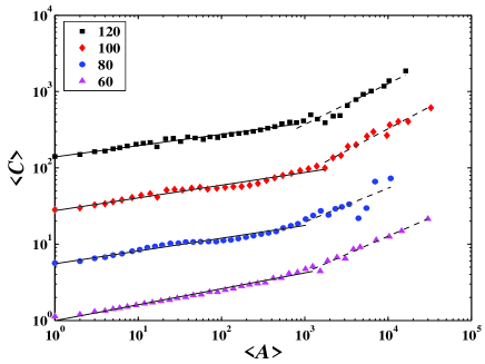
Figure 7: Plots of $\langle{C}\rangle$ with respect to $\langle{A}\rangle$ at different temperatures. The plots are translated vertically for clarity. We note that $\langle{C}\rangle=2/\pi^{1/2}$ when $\langle{A}\rangle=1$ in all the four plots.

Similarly, we can derive the relationship among $q$, $D$, $\mu_{A}$, and $\nu$ as follows

$$\nu=2\mu_{A}/(D-1)=\mu_{A}/q~{}.$$ (13)

Again, the discrepancy between the fitted $\nu$ values and those estimated indirectly from (13) is remarkable ($38\%$, $48\%$, $53\%$, $30\%$), which can also be resorted to similar reasoning.

IV Conclusion

We have investigated the fractal characteristics of the fracture surfaces of swelled isotactic polypropylene Y1600 impregnated with nucleating agent NA21 through consideration of the statistics of the islands in binary images. At a given temperature, the distributions of area and perimeter of the islands are found to follow power laws spanning over two decades of magnitude, via rank-ordering statistics. The well-established power-law scaling between area and perimeter shows the overall self-similarity among islands when $A<10^{3}$. This shows that the fracture surface is self-similar. For large islands, the fractal dimension is estimated to be close to 2 which can be explained by the fact that most of the large islands are strip-shaped. The fracture surface is rougher at low temperature with larger fractal dimension.

We have also investigated the shape complexity of the fracture surfaces using a dimensionless measure $C$. The distribution of shape complexity is also found to follow a power law spanning over two decades of magnitude. The shape complexity increases when the island is larger. There are two power-law scaling ranges between $C$ and $A$ delimited around $A=10^{3}$, corresponding to the two-regime area-perimeter relationship. The exponent $q_{1}$ serves as an inverse measure of overall shape complexity, which is observed to increases with temperature. This is consistent with the change of fractal dimension at different temperatures.

Furthermore, the relationships among different power-law scaling exponents of the probability distributions ($\mu_{A}$, $\mu_{B}$, and $\nu$), of area-perimeter relation ($D$), and of complexity-area relation ($q$) have been derived analytically. However, these relations hold only when the probability distributions of $A$, $L$, and $C$ follow exactly power laws. In the present case, we observed remarkable discrepancy between numerical and analytical results.