Wall-Fluid and Liquid-Gas Interfaces of Model Colloid-Polymer Mixtures by Simulation and Theory

Abstract

We perform a study of the interfacial properties of a model suspension of hard sphere colloids with diameter $\sigma_{c}$ and non-adsorbing ideal polymer coils with diameter $\sigma_{p}$. For the mixture in contact with a planar hard wall, we obtain from simulations the wall-fluid interfacial free energy, $\gamma_{\rm wf}$, for size ratios $q=\sigma_{p}/\sigma_{c}=0.6$ and 1, using thermodynamic integration, and study the (excess) adsorption of colloids, $\Gamma_{c}$, and of polymers, $\Gamma_{p}$, at the hard wall. The interfacial tension of the free liquid-gas interface, $\gamma_{{\rm lg}}$, is obtained following three different routes in simulations: i) from studying the system size dependence of the interfacial width according to the predictions of capillary wave theory, ii) from the probability distribution of the colloid density at coexistence in the grand canonical ensemble, and iii) for statepoints where the colloidal liquid wets the wall completely, from Young’s equation relating $\gamma_{{\rm lg}}$ to the difference of wall-liquid and wall-gas interfacial tensions, $\gamma_{\rm wl}-\gamma_{\rm wg}$. In addition, we calculate $\gamma_{\rm wf},\Gamma_{c}$, and $\Gamma_{p}$ using density functional theory and a scaled particle theory based on free volume theory. Good agreement is found between the simulation results and those from density functional theory, while the results from scaled particle theory quantitatively deviate but reproduce some essential features. Simulation results for $\gamma_{{\rm lg}}$ obtained from the three different routes are all in good agreement. Density functional theory predicts $\gamma_{{\rm lg}}$ with good accuracy for high polymer reservoir packing fractions, but yields deviations from the simulation results close to the critical point.

I Introduction

Mixtures of sterically-stabilized colloids and non-adsorbing polymers are widely studied complex fluids W. C. K. Poon (2002); Tuinier et al. (2003); J. M. Brader et al. (2003). Provided the size and the number of polymers is sufficiently high, such mixtures can phase-separate into a colloidal gas phase that is poor in colloids and rich in polymers, and a colloidal liquid phase that is rich in colloids and poor in polymers. The mechanism behind this demixing transition is of entropic origin and is due to the so-called depletion effect: An effective attraction between the colloids is generated due to an unbalanced osmotic pressure arising from exclusion of polymer coils in the depletion zones between the colloids S. Asakura and F. Oosawa (1954); A. Vrij (1976). Since the associated relevant time and length scales are much larger than in atomic and molecular systems, direct experimental observations using advanced microscopy techniques enable the study of many interesting physical phenomena, e.g. thermal capillary waves at fluid interfaces and droplet coalescence were observed recently in real space and real time using confocal microscopy D. G. A. L. Aarts et al. (2004a). Other recent examples are the direct measurement of the contact angle of the colloidal gas-liquid interface and different substrates W. K. Wijting et al. (2003a), complete wetting of a substrate D. G. A. L. Aarts et al. (2003); W. K. Wijting et al. (2003b), a wetting transition from complete to partial wetting W. K. Wijting et al. (2003b), and capillary condensation in confining geometry D. G. A. L. Aarts and H. N. W. Lekkerkerker (2004). Hence it is fair to say that these mixtures serve as excellent model systems to investigate fundamental issues in statistical physics. A particularly simple model for colloid-polymer mixtures was proposed by Vrij A. Vrij (1976), and is often referred to as the Asakura-Oosawa-Vrij (AOV) model. A good historical introduction to this model together with many recent results can be found in the paper by Brader et al. J. M. Brader et al. (2003). The bulk phase behavior as well as inhomogeneous properties of the AOV model were studied with both theory H. N. W. Lekkerkerker et al. (1992); J. M. Brader et al. (2003); D. G. A. L. Aarts et al. (2004b); P. P. F. Wessels et al. (2004a, b) and computer simulation Meijer and Frenkel (1994); M. Dijkstra et al. (1999); M. Dijkstra and R. van Roij (2002); P. G. Bolhuis et al. (2002); M. Schmidt et al. (2003, 2004); R. L. C. Vink and J. Horbach (2004a, b); R. L. C. Vink (2004). Recently, attention was paid to more realistic model interactions Dzubiella et al. (2001); P. G. Bolhuis et al. (2002); P. P. F. Wessels et al. (2004b) for colloid-polymer mixtures. However, most of the essential physics of real colloid-polymer mixtures is indeed captured by the AOV model.

In this work we study the wall-fluid and liquid-gas interfacial tensions of the AOV colloid-polymer mixture using Monte Carlo simulations and check the predictions of density functional theory (DFT) M. Schmidt et al. (2000); P. P. F. Wessels et al. (2004b) based on an extension of the Rosenfeld functional Y. Rosenfeld (1989), and of a scaled particle theory (SPT) P. P. F. Wessels et al. (2004b) based on the free volume theory H. N. W. Lekkerkerker et al. (1992). The wall-fluid interfacial tension of a hard-sphere fluid in contact with a planar hard wall was recently calculated by Heni and Löwen using a thermodynamic integration procedure along a path that corresponds to the growth of a wall in a bulk system M. Heni and H. Löwen (1999). Here, we propose a thermodynamic integration approach similar in spirit, to determine the wall-fluid interfacial free energy of the AOV colloid-polymer mixture in contact with a planar hard wall.

Different routes exist to determine the liquid-gas interfacial tension. The pressure tensor method J. R. Henderson and F. van Swol (1984); H. Heinz et al. (2004) is particularly suitable for Molecular Dynamics simulation studies. The probability distribution method K. Binder (1982) was used in Monte-Carlo simulations J. J. Potoff and A. Z. Panagiotopoulos (2000); M. Müller and L. G. MacDowell (2003) and was recently applied to calculate the liquid-gas interfacial tension of colloid-polymer mixtures R. L. C. Vink and J. Horbach (2004a, b); R. L. C. Vink (2004); Vink et al. (2004a). The authors showed that the interfacial width depends on system size and they verified the predictions from capillary wave theory on system size dependence R. L. C. Vink and J. Horbach (2004b). Sides et al. and Lacasse et al. found good agreement between the interfacial tension obtained from the pressure tensor method and from the predictions of capillary wave theory provided that the density profile is fit to an error function for Lennard-Jones particles and polymer blends S. W. Sides et al. (1999); M.-D. Lacasse et al. (1998). In this work, we use both the capillary wave theory, as proposed in Refs. S. W. Sides et al. (1999); M.-D. Lacasse et al. (1998), as well as the probability distribution method to calculate the liquid-gas interfacial tension. In addition, we employ Young’s equation in the complete wetting regime to obtain an estimate for the tension of the liquid-gas interface from the difference in wall tensions, and compare our results with DFT calculations.

The paper is organized as follows. In section II we briefly review the AOV model. In section III.1 an overview of the thermodynamics of inhomogeneous systems is given. In section III.2 we lay out the simulation methods used in the determination of the wall-fluid tension. Section III.3 details the simulation method to obtain the adsorption at a hard wall. Section III.4 presents the corresponding derivation using scaled particle theory. In section III.5 we review the capillary wave theory for the width of a liquid-gas interface. Sections III.6 and III.7 are devoted to obtaining the liquid-gas interfacial tension from the probability distribution of the colloid density at coexistence and from Young’s equation, respectively. Section III.8 gives a brief overview of the DFT. In section IV we discuss our results for the wall-fluid tension (IV.1), adsorption (IV.2), and liquid-gas interfacial tension (IV.3). Concluding remarks are given in section V.

II Model

We consider a mixture of sterically-stabilized colloidal spheres (species $c$) and non-adsorbing polymer coils (species $p$) immersed in a solvent. The interaction between two sterically stabilized colloids resembles closely that of hard spheres, while a dilute solution of polymer coils in a theta-solvent can be treated as an ideal gas as the polymer coils are interpenetrable and noninteracting. The polymer coils are assumed to be excluded from the colloids to a center-of-mass distance of $(\sigma_{c}+\sigma_{p})/2$, where $\sigma_{c}$ is the diameter of the colloids, and $\sigma_{p}=2R_{g}$ is the diameter of the polymer coils, with $R_{g}$ being the radius of gyration of the polymers. A simple idealized model for such a mixture is the so-called Asakura-Oosawa-Vrij (AOV) model S. Asakura and F. Oosawa (1954); A. Vrij (1976) defined through pair potentials, that between colloids being

$$v_{cc}(R_{ij})=\left\{\begin{array}[]{ll}\infty&\textrm{ if $R_{ij}<\sigma_{c}$ }\\ 0&\textrm{ otherwise,}\end{array}\right.$$ (1)

where $R_{ij}=|\vec{R}_{i}-\vec{R}_{j}|$ is the center-of-mass distance between two colloidal particles, with $\vec{R}_{i}$ ($\vec{R}_{j}$) the center-of-mass coordinate of colloid $i$ ($j$). The polymers are described as noninteracting particles with

$$v_{pp}(r_{ij})=0,$$ (2)

where $r_{ij}=|\vec{r}_{i}-\vec{r}_{j}|$ is the distance between two polymers, with $\vec{r}_{i}$ ($\vec{r}_{j}$) the center-of-mass coordinate of polymer $i$ ($j$). The colloid-polymer interaction is

$$v_{cp}(|\vec{R}_{i}-\vec{r}_{j}|)=\left\{\begin{array}[]{ll}\infty&\textrm{ if $|\vec{R}_{i}-\vec{r}_{j}|<(\sigma_{c}+\sigma_{p})/2$ }\\ 0&\textrm{ otherwise,}\end{array}\right.$$ (3)

where $|\vec{R}_{i}-\vec{r}_{j}|$ is the distance between colloid $i$ and polymer $j$. Our simulations are performed in a box with dimensions $L\times L\times H$ with three-dimensional periodic boundary conditions in the case of bulk simulations. To create a wall-fluid or a liquid-gas interface, we perform simulations in a box with periodic boundary condition solely in the $x$ and $y$ directions and two impenetrable hard walls in the $z$ direction. The wall-particle potential acting on particles of species $k=c,p$ reads

$$v_{wk}(z_{k,i})=\left\{\begin{array}[]{ll}0&\textrm{ if $\sigma_{k}/2<z_{k,i}<H_{k}-\sigma_{k}/2$ }\\ \infty&\textrm{ otherwise}\end{array}\right.,$$ (4)

where $z_{k,i}$ is the $z$-coordinate of particle $i$ of species $k$, and $H_{k}$ is the separation distance between the two walls for species $k$. For the simulations of hard wall properties, we use $H_{c}=H_{p}\equiv H$, corresponding to two planar hard walls. For the simulations of the liquid-gas interface we use a box with periodic boundary conditions in the $x$ and $y$ directions and delimited in the $z$ direction by one impenetrable and one semi-permeable wall; this asymmetric slit is defined by the wall-particle potential (4) with $H_{c}=H-2\sigma_{c}$ and $H_{p}=H$. The impenetrable wall at $z=0$ favors the colloidal liquid phase, while the semi-permeable wall at $z=H_{c}$ is impenetrable for the colloidal particles, but penetrable for the polymers (which are free to overlap with this wall). Hence, there is no effective polymer-mediated wall-colloid attraction and the semi-permeable wall favors the colloidal gas phase M. Dijkstra and R. van Roij (2002); M. Schmidt et al. (2003, 2004); P. P. F. Wessels et al. (2004b).

The size ratio $q=\sigma_{p}/\sigma_{c}$ is a geometric parameter that controls the range of the effective depletion interaction between the colloids. Packing fraction are denoted by $\eta_{k}=(\pi\sigma_{k}^{3}N_{k})/(6L^{2}H)$, and the number density is denoted by $\rho_{k}=N_{k}/(L^{2}H)$ for species $k=c,p$. We also employ, as an alternative thermodynamic variable to $\eta_{p}$, the polymer reservoir packing fraction

$$\eta_{p}^{r}=\frac{\pi}{6}\sigma_{p}^{3}\rho_{p}^{r}=\frac{\pi}{6}\sigma_{p}^{3}z_{p},$$ (5)

where $z_{p}$ is the fugacity of the polymers, that constitute an ideal gas with density $\rho_{p}^{r}$ in the reservoir.

III Methods

III.1 Overview of interfacial thermodynamics

Generally, the interfacial tension in an inhomogeneous system is the grand potential per unit area needed to create an interface in an initially uniform bulk system at fixed chemical potential of colloids, $\mu_{c}$, and polymers, $\mu_{p}$, and fixed volume $V$ and temperature $T$. The grand potential for a bulk mixture of colloids and polymers reads

$$\Omega^{\rm bulk}(\mu_{c},\mu_{p},V,T)=-p(\mu_{c},\mu_{p},T)V,$$ (6)

where $p$ is the bulk pressure. The system in contact with an interface possesses the grand potential

$$\Omega(\mu_{c},\mu_{p},V,T,A)=-p(\mu_{c},\mu_{p},T)V+\gamma(\mu_{c},\mu_{p},T)A,$$ (7)

where $A$ is the area of the interface and $\gamma(\mu_{c},\mu_{p},T)$ is the interfacial tension, which can hence be expressed as

$$\gamma=\frac{\Omega(\mu_{c},\mu_{p},V,T,A)-\Omega^{\rm bulk}(\mu_{c},\mu_{p},V,T)}{A}.$$ (8)

Besides the liquid-gas interface, where $\gamma=\gamma_{\rm lg}$, Eqs. (6), (7), and (8) apply also for a fluid adsorbed between two parallel plates (walls), where $\gamma=\gamma_{\rm wf}$, provided that the wall separation is sufficiently large R. Evans and U. Marini Bettolo Marconi (1987); M. Dijkstra (1997), and that the area $A$ is equal to the total area of the two plates, $A=2L^{2}$. At fixed chemical potentials the number of particles in the inhomogeneous system, $N_{c}$ and $N_{p}$, of colloids and polymers, respectively, will be in general different from those in the bulk, $N_{c}^{\rm bulk}$ and $N_{p}^{\rm bulk}$. The excess number of colloids and polymers per unit area, i.e. the adsorptions $\Gamma_{c}$ and $\Gamma_{p}$, respectively, are defined as

$$\Gamma_{c}(\mu_{c},\mu_{p},T) = \frac{N_{c}-N_{c}^{\rm bulk}}{A},$$ (9)

$$\Gamma_{p}(\mu_{c},\mu_{p},T) = \frac{N_{p}-N_{p}^{\rm bulk}}{A}.$$ (10)

The grand potentials (6) and (7) in differential form read

$$d\Omega^{\rm bulk}(\mu_{c},\mu_{p},V,T) = -N_{c}^{\rm bulk}d\mu_{c}-N_{p}^{\rm bulk}d\mu_{p}-pdV-S^{\rm bulk}dT,,$$ (11)

$$d\Omega(\mu_{c},\mu_{p},V,T,A) = -N_{c}d\mu_{c}-N_{p}d\mu_{p}-pdV-SdT+\gamma dA.$$ (12)

Using Eqs. (11) and (12) and Eq. (8) in differential form, it is straightforward to show J. S. Rowlinson and B. Widom (2002) that the adsorptions are related to the interfacial tension through

$$\Gamma_{c}=-\left(\frac{\partial\gamma}{\partial\mu_{c}}\right)_{\mu_{p},T}\hskip 14.22636pt\mbox{and}\hskip 14.22636pt\Gamma_{p}=-\left(\frac{\partial\gamma}{\partial\mu_{p}}\right)_{\mu_{c},T}.$$ (13)

III.2 Hard wall-fluid interfacial tension via thermodynamic integration

To determine, from simulations, the wall-fluid tension $\gamma_{\rm wf}$ of the AOV model we should apply equation (8), as is manifest in the grand canonical ensemble, i.e. for constant colloid and polymer fugacities. However, in our simulation it is more convenient to use the semi-grand canonical ensemble fixing the number of colloids and the fugacity of the polymers. The reason is twofold. First the interfacial tension as a function of the fugacity of polymers can be directly compared to the DFT results of Ref. P. P. F. Wessels et al. (2004b). Second, fixing the number of colloids instead of their fugacity allow us to efficiently study state points with high packing fractions of colloids; generally grand ensemble simulations are difficult to perform at high densities due to small particle insertion probabilities. To compute the tension we have to recast Eq. (8) in a way that is consistent with the semi-grand canonical ensemble. The grand potentials for the bulk and the inhomogeneous system are related to the corresponding Helmholtz free energies via a Legendre transformation,

$$\Omega^{\rm bulk}(\mu_{c},\mu_{p},V,T) = F^{\rm bulk}(N_{c}^{\rm bulk},N_{p}^{\rm bulk},V,T)-\mu_{c}N_{c}^{\rm bulk}-\mu_{p}N_{p}^{\rm bulk},$$ (14)

$$\Omega(\mu_{c},\mu_{p},V,T,A) = F(N_{c},N_{p},V,T,A)-\mu_{c}N_{c}-\mu_{p}N_{p}.$$ (15)

We substitute Eqs. (14) and (15) in Eq. (8) to obtain

$$\gamma=\frac{F(N_{c},N_{p})-F^{\rm bulk}(N_{c}^{\rm bulk},N_{p}^{\rm bulk})}{A}-\mu_{c}\Gamma_{c}-\mu_{p}\Gamma_{p},$$ (16)

where we omitted the dependence on the variables $V,T,\mu_{c},$ and $\mu_{p}$ in the notation. Note that the tension is not only the difference of the Helmholtz free energies, but additional terms, $\mu_{c}\Gamma_{c}$ and $\mu_{p}\Gamma_{p}$, arise in Eq. (16). One can further simplify by Taylor expanding $F(N_{c},N_{p},V,T,A)$ around $N_{c}^{\rm bulk}$:

$$F(N_{c},N_{p},V,T,A)=F(N_{c}^{\rm bulk},N_{p},V,T,A)+\frac{\partial F}{\partial N_{c}}(N_{c}-N_{c}^{\rm bulk})+\mathcal{O}((N_{c}-N_{c}^{\rm bulk})^{2}).$$ (17)

Keeping only the first order term, one can approximate the interfacial tension as

$$\gamma\simeq\frac{F(N_{c}^{\rm bulk},N_{p},V,T,A)-F^{\rm bulk}(N_{c}^{\rm bulk},N_{p}^{\rm bulk},V,T)}{A}-\mu_{p}\Gamma_{p}.$$ (18)

The same approximation was employed in Ref. M. Heni and H. Löwen (1999) (using $N_{p}=0$ and $N_{p}^{\rm bulk}=0$) to calculate the interfacial free energy of hard spheres in contact with a planar hard wall. To compute the wall tension, we need to perform two free energy calculations, one for the bulk and one for the inhomogeneous system. As the free energy cannot be measured directly in a Monte Carlo simulation, we use the thermodynamic integration techniqueD. Frenkel and B. Smit (2002) to relate the free energy of the system of interest to that of a reference system

$$F(N_{c},N_{p},V,T,A,\lambda=\lambda_{\rm max})=F_{id}(N_{c},N_{p},V,T,\lambda=0)+\int_{\lambda=0}^{\lambda_{\rm max}}d\lambda\left\langle\frac{\partial F}{\partial\lambda}\right\rangle_{\lambda}.$$ (19)

The reference system is chosen to be an ideal gas, so $F_{id}(N_{c},N_{p},V,T,\lambda=0)$ is the Helmholtz free energy of $N_{c}$ ideal colloids and $N_{p}$ ideal polymers in a volume $V$ at temperature $T$. We then introduce the suitable auxiliary Hamiltonian

$$H_{\lambda}=\lambda\left(\sum_{i<j}^{N_{c}}V_{cc}(R_{ij})+\sum_{i=1}^{N_{c}}\sum_{j=1}^{N_{p}}V_{cp}(|\vec{R}_{i}-\vec{r}_{j}|)+\epsilon\sum_{i=1}^{N_{c}}V_{wc}(z_{c,i})+\epsilon\sum_{i=1}^{N_{p}}V_{wp}(z_{p,i})\right),$$ (20)

where we approximate the hard-core potentials of the AOV model with penetrable potentials: The colloid-colloid interaction reads

$$V_{cc}(R_{ij})=\Theta(\sigma_{c}-R_{ij}),$$ (21)

where $\Theta(x)$ is the Heaviside step function. Likewise we define the interaction potential between the colloids and the polymers as

$$V_{cp}(|\vec{R}_{i}-\vec{r}_{j}|)=\Theta\left(\frac{(\sigma_{c}+\sigma_{p})}{2}-|\vec{R}_{i}-\vec{r}_{j}|\right).$$ (22)

The interaction between the walls and the particles of species $k=c,p$ is

$$V_{wk}(z_{k,i})=\Theta\left(\frac{\sigma_{k}}{2}-z_{k,i}\right)+\Theta\left(\frac{\sigma_{k}}{2}-(H_{k}-z_{k,i})\right),$$ (23)

where $z_{k,i}$ is the $z$-coordinate of particle $i$ of species $k$. For $\lambda=0$, this system reduces to an ideal gas, while for $\lambda\rightarrow\infty$, the system describes the AOV model given by Eqs. (1)-(4) in bulk ($\epsilon=0$) or confined by two walls ($\epsilon=1$). The interaction potential is switched on adiabatically using the coupling parameter $\lambda$. In principle, our system of interest is described by the Hamiltonian (20) using $\lambda_{\rm max}\rightarrow\infty$, but also for sufficiently high values of $\lambda_{\rm max}$ the system reduces to our system of interest with hard-core potentials. Clearly, $\lambda_{\rm max}$ should be sufficiently large to ensure that the system is indeed behaving as the hard-core system of interest. On the other hand, $\lambda_{\rm max}$ should not be too large, as this would make the numerical integration less accurate. The integrand function of Eq. (19) is then

$$\left\langle\frac{\partial F}{\partial\lambda}\right\rangle_{\lambda}=\left\langle\frac{\partial H_{\lambda}}{\partial\lambda}\right\rangle_{\lambda}=\left\langle\frac{H_{\lambda}}{\lambda}\right\rangle_{\lambda}.$$ (24)

The function $\left\langle\frac{H_{\lambda}}{\lambda}\right\rangle_{\lambda}$ is computed counting the number of overlaps between colloids, colloids and polymers and (for the inhomogeneous system only) particles and walls. The free energy can then be obtained using Eq. (19). The integrals are evaluated using a 21-point Gauss-Kronrod formula, where 5000-15000 MC cycles per particle are used for the sampling of each integration point. The wall-fluid interfacial tension is then computed using equation (18). In detail, we first perform a simulation of the AOV model in bulk and a separate simulation of the AOV model confined by two walls, given by the interactions (1)-(4), both in the semi-grand canonical ensemble, i.e., we fix the number of colloids $N_{c}^{\rm bulk}$, the chemical potential of the polymers $\mu_{p}$, and the volume $V=L\times L\times H$. We measure the average number of polymer in the bulk, $\langle N_{p}^{\rm bulk}\rangle$, and in the confined system, $\langle N_{p}\rangle$. We then perform two separate thermodynamic integrations (in the canonical ensemble) to obtain the free energy of the bulk system with $N_{c}^{\rm bulk}$ colloids and $\langle N_{p}^{\rm bulk}\rangle$ polymers in a volume $V$, and the confined system of volume $V$ with $N_{c}^{\rm bulk}$ colloids and $\langle N_{p}\rangle$ polymers. In the canonical ensemble simulations, we determined the chemical potential of the polymer as a consistency check. Typical number of the colloids and the polymers are $N_{c}^{\rm bulk}=54-900$ and $N_{p}^{\rm bulk}=0-20000$, while the volume of the simulation box is about $V=(1200-3000)\sigma_{c}^{3}$ and $H>16\sigma_{c}$. The errors are estimated calculating the standard deviation from 4 or 5 independent simulations.

III.3 Adsorption at a hard wall from simulation

To study the (excess) adsorption of colloid-polymer mixtures at a planar hard wall we simulated both the bulk mixture and the mixture in contact with the hard wall in two independent Monte Carlo simulations in the grand canonical ensemble ensemble and hence we considered only statepoints of low colloid packing fraction $\eta_{c}$. After discarding 50000 MC steps per particle for equilibration, we take the average of the number of particles for another 50000 MC steps per particle. The differences in particle numbers (per unit area) in the confined system and in the bulk system then give the adsorption of both species via Eqs. (9) and (10).

III.4 Adsorption at a hard wall from scaled-particle theory

For a system of hard spheres the scaled particle theory H. Reiss et al. (1959, 1960) describes quite accurately the pressure $p$, the hard wall-fluid interfacial tension $\gamma_{\rm hs}$, and the (excess) adsorption $\Gamma_{\rm hs}$, given through the expressions

$$\frac{\beta p}{\rho_{c}} = \frac{1+\eta_{c}+\eta_{c}^{2}}{(1-\eta_{c})^{3}},$$ (25)

$$\beta\gamma_{\rm hs}\sigma_{c}^{2} = 3\eta_{c}\frac{(2+\eta_{c})}{2\pi(1-\eta_{c})^{2}},$$ (26)

$$\Gamma_{\rm hs}\sigma_{c}^{2} = \frac{9\eta_{c}^{2}}{\pi(1+2\eta_{c})}-\frac{3\eta_{c}}{\pi}.$$ (27)

In particular, Eq. (27) was shown to compare well with simulation J. R. Henderson and F. van Swol (1984) and DFT R. Roth and S. Dietrich (2000) results.

Recently an SPT expression for the wall-fluid tension of AOV model colloid-polymer mixtures was derived by Wessels et al. P. P. F. Wessels et al. (2004b) using the bulk free energy for a ternary mixture obtained from free volume theory H. N. W. Lekkerkerker et al. (1992) as an input, and taking the limit of vanishing concentration and infinite size of the third component. Their expression reads

$$\beta\gamma_{\rm wf}\sigma_{c}^{2}=\beta\gamma_{\rm hs}\sigma_{c}^{2}+\eta_{p}^{r}f(\eta_{c}),$$ (28)

where $f(\eta_{c})=3\alpha(\eta_{c})/(q^{2}\pi)[1+(1+3q+q^{2})\tau+(3q+4q^{2})\tau^{2}+3q^{2}\tau^{3}]$, $\tau=\eta_{c}/(1-\eta_{c})$ and $\beta\gamma_{\rm hs}\sigma_{c}^{2}$ is given by equation (26). The polymer free volume is given by the scaled particle theory as $\alpha(\eta_{c})=(1-\eta_{c})\exp(-(3q+3q^{2}+q^{3})\tau-(9q^{2}/2+3q^{3})\tau^{2}-3q^{3}\tau^{3})$. Results for $\gamma_{\rm wf}$ from equation (28) were found in Ref. P. P. F. Wessels et al. (2004b) to compare reasonably well with those from full numerical density functional calculations. Below we will compare these approaches against our simulation data.

Here we derive an SPT expression for the adsorption of the AOV model at a hard wall starting from equation (28) and building derivatives according to (13). The colloid chemical potential obtained from the free volume theory H. N. W. Lekkerkerker et al. (1992) is

$$\beta\mu_{c}=\beta\mu_{\rm hs}(\eta_{c})-\eta_{p}^{r}\frac{\alpha^{{}^{\prime}}}{q^{3}},$$ (29)

where $\beta\mu_{\rm hs}(\eta_{c})=\eta_{c}(14-13\eta_{c}+5\eta_{c}^{2})/(2(1-\eta_{c})^{3})-\log(1-\eta_{c})+\log(6\eta_{c}/\pi)$ is the SPT expression of the chemical potential of a system of pure hard spheres at packing fraction $\eta_{c}$ and $\alpha^{{}^{\prime}}=\partial\alpha/\partial\eta_{c}$. We compute the colloidal adsorption using equation (13)

$$\Gamma_{c}\sigma_{c}^{2}=-\frac{\partial\beta\gamma_{\rm wf}(\mu_{c},\mu_{p})\sigma_{c}^{2}}{\partial\beta\mu_{c}}=-\frac{\partial\beta\gamma_{\rm wf}(\eta_{c},\mu_{p})\sigma_{c}^{2}}{\partial\eta_{c}}\frac{\partial\eta_{c}}{\partial\beta\mu_{c}},$$ (30)

where

$$\frac{\partial\eta_{c}(\mu_{c},\mu_{p})}{\partial\beta\mu_{c}}=\left(\frac{\partial\beta\mu_{c}(\eta_{c},\mu_{p})}{\partial\eta_{c}}\right)^{-1},$$ (31)

is computed using equation (29). The final expression is

$$\Gamma_{c}\sigma_{c}^{2}=\Gamma_{\rm hs}\sigma_{c}^{2}\left(\frac{1+\eta_{p}^{r}\frac{f^{{}^{\prime}}}{\beta\gamma_{\rm hs}^{{}^{\prime}}\sigma_{c}^{2}}}{1-\eta_{p}^{r}\frac{\alpha^{{}^{\prime\prime}}}{\beta\mu_{\rm hs}^{{}^{\prime}}q^{3}}}\right),$$ (32)

where $f^{{}^{\prime}}=\partial f/\partial\eta_{c}$, $\gamma_{\rm hs}^{{}^{\prime}}=\partial\gamma_{\rm hs}/\partial\eta_{c}$, $\mu_{\rm hs}^{{}^{\prime}}=\partial\mu_{\rm hs}/\partial\eta_{c}$ and $\alpha^{{}^{\prime\prime}}=\partial^{2}\alpha/\partial\eta_{c}^{2}$. We note that the hard-sphere limit is obtained correctly for $\eta_{p}^{r}=0$. We also calculate the polymer adsorption

$$\Gamma_{p}\sigma_{c}^{2}=-\frac{\partial\beta\gamma_{\rm wf}(\eta_{c},\mu_{p})\sigma_{c}^{2}}{\partial\beta\mu_{p}}=-\eta_{p}^{r}f-\left(\frac{\partial\beta\gamma_{\rm hs}(\eta_{c})\sigma_{c}^{2}}{\partial\eta_{c}}+\eta_{p}^{r}\frac{\partial f(\eta_{c})}{\partial\eta_{c}}\right)\frac{\partial\eta_{c}}{\partial\beta\mu_{p}}.$$ (33)

Rewriting Eq. (29) as

$$\eta_{p}^{r}=\frac{\beta\mu_{\rm hs}(\eta_{c})-\beta\mu_{c}}{\alpha^{{}^{\prime}}}q^{3},$$ (34)

we arrive at

$$\frac{\partial\eta_{c}}{\partial\beta\mu_{p}}=\eta_{p}^{r}\left(\frac{\partial\eta_{p}^{r}}{\partial\eta_{c}}\right)^{-1}=\frac{\eta_{p}^{r}\alpha^{\prime}}{q^{3}\beta\mu_{\rm hs}^{\prime}-\eta_{p}^{r}\alpha^{{}^{\prime\prime}}}.$$ (35)

The final expression reads

$$\Gamma_{p}(\eta_{c})\sigma_{c}^{2}=-(\beta\gamma_{\rm wf}-\beta\gamma_{\rm hs})\sigma_{c}^{2}+\eta_{p}^{r}\frac{\alpha^{{}^{\prime}}}{q^{3}}\Gamma_{c}(\eta_{c})\sigma_{c}^{2}.$$ (36)

III.5 Liquid-gas interfacial tension from capillary wave broadening

Capillary wave theory describes the broadening of an intrinsic interface of width $w_{0}$ due to thermal fluctuations. This broadening depends primarily on the interfacial tension and the area of the interface. To calculate the capillary wave contribution to the interfacial width one has to sum over the contributions from each thermally excited capillary wave to the amplitude of the oscillations in the instantaneous interface position. Here we briefly sketch the derivation of Sides et al. and Lacasse et al. and refer the reader to Refs. S. W. Sides et al. (1999); M.-D. Lacasse et al. (1998) for further details; a very recent study devoted to capillary waves in colloid-polymer mixtures is that by Vink et al. Vink et al. (2004b). Fluctuations due to capillary waves in $\zeta(x,y)$, the mean location of the interface in the $z$-direction, have an energy cost due to the increase in surface area of the interface. The free energy cost of the interfacial fluctuations is the product of the excess area of the undulated interface over that of the flat one, and a liquid-gas interfacial tension $\gamma_{{\rm lg}}$, which is assumed to be independent of curvature. The interfacial Hamiltonian, assuming that $\zeta$ and its derivatives are small, reads

$${\cal H}=\frac{\gamma_{{\rm lg}}}{2}\int dxdy|\nabla\zeta(x,y)|^{2}.$$ (37)

Introducing a Fourier expansion of $\zeta(x,y)$, one arrives at

$$\cal{H} = \frac{\gamma_{{\rm lg}}}{2}\int d\vec{q}q^{2}|\tilde{\zeta}(\vec{q})|^{2},$$ (38)

where $\vec{q}=(q_{x},q_{y})$ denotes a two-dimensional wavevector and $\tilde{\zeta}(\vec{q})$ is the Fourier transform of $\zeta(x,y)$. Using the equipartition theorem, the mean-square amplitude for each interfacial excitation mode reads

$$\langle|\tilde{\zeta}(\vec{q})|^{2}\rangle=\frac{k_{B}T}{\gamma_{{\rm lg}}q^{2}}.$$ (39)

The mean-squared real space fluctuations can be calculated by summing over all allowed modes:

$$\langle|\zeta(x,y)|^{2}\rangle = \frac{1}{(2\pi)^{2}}\int_{q_{\rm min}}^{q_{\rm max}}d\vec{q}\langle|\zeta(\vec{q})|^{2}\rangle$$ (40)

$$= \frac{k_{B}T}{2\pi\gamma_{{\rm lg}}}\ln\left(\frac{L}{\xi_{b}}\right),$$

where the low $q$ cutoff, $q_{\rm min}$, is determined by the system size, i.e., $q_{\rm min}=2\pi/L$ in our simulations and gives rise to system size dependence. The high $q$ cutoff, $q_{\rm max}=2\pi/\xi_{b}$, is determined by the bulk correlation length $\xi_{b}$, which is of the order of the colloid diameter, and avoids the divergence in the integral.

The total width of the interface, as measured in experiments and simulations, includes contributions from the intrinsic width and the broadening due to capillary wave fluctuations. If one assumes that the capillary-wave fluctuations are decoupled from the intrinsic profile, the total interfacial profile $\Psi(z)$ can be expressed as a convolution of the intrinsic interfacial profile $\psi(z)$ and the fluctuations due to capillary waves

$$\Psi(z)=\int_{-\infty}^{\infty}\psi(z-z_{0})P(z_{0})dz_{0},$$ (41)

where $P(z_{0})$ is the probability of finding the local interface at $z_{0}$. The interfacial order parameter profile $\Psi(z)$ is defined such that it varies between -1 and 1

$$\Psi(z)=\frac{2}{\rho_{c}^{l}-\rho_{c}^{g}}\left[\rho_{c}(z)-\frac{\rho_{c}^{l}+\rho_{c}^{g}}{2}\right],$$ (42)

where $\rho_{c}(z)$ is the cross-section averaged density profile of the colloids and $\rho_{c}^{l}$ and $\rho_{c}^{g}$ are the colloid densities of the colloidal ”liquid” and ”gas” phase at coexistence. In Ref. S. W. Sides et al. (1999); M.-D. Lacasse et al. (1998), the authors define the variance of the derivative of the total interfacial profile $d\Psi(z)/dz\equiv\Psi^{\prime}$ as a measure of the width of the interface. The variance of a distribution $f$ reads

$$v[f]=\frac{\int_{-\infty}^{\infty}z^{2}f(z)dz}{\int_{-\infty}^{\infty}f(z)dz}=\frac{-(d^{2}/dq^{2})\tilde{f}(q)|_{q=0}}{\tilde{f}(0)},$$ (43)

where $\tilde{f}(q)$ is the Fourier transform of $f(z)$. Using this choice of measure for the interfacial width, one can show explicitly using the convolution theorem that the total interfacial width can be written as the sum of an intrinsic part and a contribution due to capillary wave fluctuations

$$v[\Psi^{\prime}] = v[\psi^{\prime}]+v[P]$$ (44)

$$= v[\psi^{\prime}]+\frac{k_{B}T}{2\pi\gamma_{{\rm lg}}}\ln\left(\frac{L}{\xi_{b}}\right),$$

where we identify $v[P]$ as the mean-squared fluctuations due to capillary waves, i.e., $\langle|\zeta(x,y)|^{2}\rangle$.

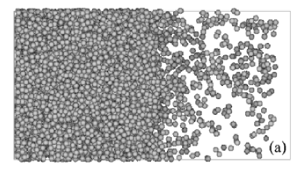
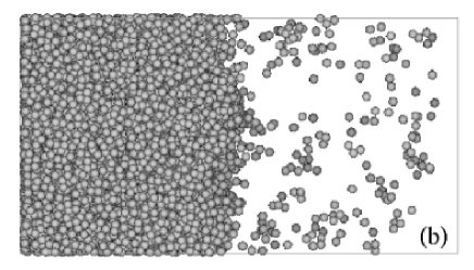
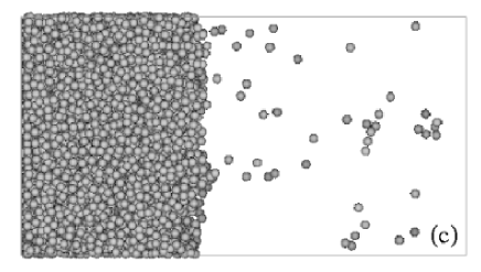
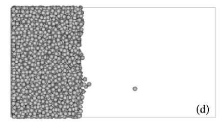
Figure 6: Typical snapshots of the colloid coordinates, obtained from Monte-Carlo simulations based on the exact effective one-component Hamiltonian for the colloids, of the liquid-gas interface of the model colloid-polymer mixture with size ratio $q=1$ and a) polymer reservoir packing fraction $\eta_{p}^{r}=0.95$; b) $\eta_{p}^{r}=1.05$; c) $\eta_{p}^{r}=1.4$; d) $\eta_{p}^{r}=2$.

To measure the tension using the results of capillary wave theory one needs to create a liquid-gas interface in the simulation box. To stabilize the liquid-gas interface we perform the simulations in a box with dimensions $L\times L\times H$, with $H=48\sigma_{c}$, delimited in the $z$ direction by one impenetrable wall and one semi-permeable wall. We vary the lateral dimensions in the range of $5\sigma_{c}<L<25\sigma_{c}$. The canonical simulations are started in the middle of the two-phase region. After equilibration the system is phase separated, the gas phase in contact with the semi-permeable wall and the liquid phase in contact with the hard-wall. The liquid-gas interface is in the middle of the simulation box (see also Fig. 6). We determine the total interfacial width $v[\Psi^{\prime}]$ from the interfacial order parameter profile $\Psi(z)$ measured in simulations according to Eq. (42). A priori, it is not clear whether the density profile should be fit to an error function or a hyperbolic tangent. In Ref. S. W. Sides et al. (1999), it is shown explicitly that the interfacial width extracted through fits of the density profile to a hyperbolic tangent lead to systematic errors and that better results for the interfacial tensions are obtained using the error function. In addition, later work on water/carbon tetrachloride S. Senapati and M. L. Berkowitz (2001) and molten salt (KI) A. Aguado et al. (2001) interfaces also found good agreement between the interfacial tension calculated using the capillary wave formalism and the pressure tensor components. Fitting $\Psi(z)$ by an error function $\mbox{erf}[(z-z_{0})/(w\sqrt{2})]$, using $z_{0}$ and $w$ as fitting parameters, we find that the variance of the derivative of this fitting function is related to the interfacial width $w$, i.e., $v[\Psi^{\prime}]=w^{2}$. Using Eq. (44) we are able to determine $\gamma_{{\rm lg}}$ from the fits of the size dependence of the interfacial width.

In contrast to the wall-fluid tension and the adsorption simulations described in section III.2 and III.3, we used for the liquid-gas interfacial tension simulations described in this section and in section  III.6, an efficient simulation scheme for the AOV model that was recently developed  M. Dijkstra and R. van Roij (2002). It is based on the exact effective one-component Hamiltonian of the colloids, i.e., it incorporates all the effective polymer-mediated many-body interactions. The effective one-component Hamiltonian can be derived by integrating out the polymer degrees of freedom in the binary colloid-polymer mixture. To this end, we consider $N_{c}$ colloids and $N_{p}$ polymer coils in a macroscopic volume $V$ at temperature $T$. The total Hamiltonian consists of interaction terms $H=H_{cc}+H_{cp}+H_{pp}$, where $H_{cc}=\sum_{i<j}^{N_{c}}v_{cc}(R_{ij})$, $H_{cp}=\sum_{i}^{N_{c}}\sum_{j}^{N_{p}}v_{cp}(|{\bf R}_{i}-{\bf r}_{j}|)$, and $H_{pp}=\sum_{i<j}^{N_{p}}v_{pp}(r_{ij})$. It is convenient to consider the system in the $(N_{c},z_{p},V,T)$ ensemble, in which the polymer fugacity is fixed. The thermodynamic potential $F$ of this system can be written as $\exp[-\beta F]=\mbox{Tr}_{c}\exp[-\beta H_{eff}]$, where $H_{eff}=H_{cc}+\Omega$ is the effective Hamiltonian and where $\mbox{Tr}_{c}$ is short for $1/N_{c}!\Lambda_{c}^{3N_{c}}$ times the volume integral over the coordinates of the colloids, and where $\Lambda_{c}$ is the thermal wavelength. It is straightforward to show that one obtains for the present model the exact result $\beta\Omega=-z_{p}V_{f}$, with the so-called free volume $V_{f}$, i.e., the accessible volume for the center-of-mass of the polymer coils. This free volume can be calculated numerically on a smart grid for each static colloid configuration. For more details, we like to refer the reader to Ref.  M. Dijkstra and R. van Roij (2002); Dijkstra et al. . The advantage of this scheme is that the polymer degrees of freedom are integrated out and enter the effective one-component colloid Hamiltonian only by the polymer reservoir packing fraction $\eta_{p}^{r}$. Hence, we avoid equilibration and statistical accuracy problems due to fluctuating polymer numbers. Moreover, our simulations are not limited by the total number of polymers and can be performed at high polymer reservoir packing fractions far away from the critical point.

III.6 Liquid-gas interfacial tension from the probability distribution

In addition, we determine $\gamma_{{\rm lg}}$ using the probability distribution method. We perform Monte-Carlo simulations in the grand canonical ensemble using again our novel effective one-component simulation scheme M. Dijkstra and R. van Roij (2002), explained in Sec.  III.5 . To obtain the probability $P(N_{c})|_{z_{c},\eta_{p}^{r}}$ of observing $N_{c}$ colloids in a volume $V$ at fixed colloid fugacity $z_{c}$ and fixed polymer reservoir packing fraction $\eta_{p}^{r}$, we use a sampling technique called successive umbrella sampling P. Virnau and M. Müller (2004). Employing this technique, we sample the probability distribution $P(N_{c})|_{z_{c},\eta_{p}^{r}}$ in small windows one after the other, in which the number of colloids $N_{c}$ is allowed to fluctuate between 0 and 1 in the first window, 1 and 2 in the second window, etc. We first perform an exploratory short run without a bias, yielding $P(N_{c}-1)$ and $P(N_{c})$ for window $N_{c}$. We then perform a biased simulation in which we sample from a non-physical distribution $\pi(N_{c})=g(N_{c})P(N_{c})$ instead of the grand canonical distribution $P(N_{c})$. We have chosen the weight function $g(N_{c})=1/P(N_{c})$, where we use $P(N_{c})$ obtained from the unbiased exploratory simulation run. This choice for the weight function yields a constant constant $\pi(N_{c})$ and the system will visit equally the state with $N_{c}-1$ colloids as the state with $N_{c}$ colloids. Of course, we have to correct our weighted sampling for the bias by dividing out the weight function $g(N_{c})$. The more accurate grand canonical distribution $P(N_{c})$ is obtained from

$$P(N_{c})=\frac{\pi(N_{c})}{g(N_{c})}.$$ (45)

In addition, we use the histogram reweighting technique to obtain the probability distribution for any $z_{c}^{\prime}$ once $P(N_{c})|_{z_{c},\eta_{p}^{r}}$ is known for a given $z_{c}$ Vink et al. (2004a):

$$P(N_{c})|_{z_{c}^{\prime},\eta_{p}^{r}}=\ln P(N_{c})|_{z_{c},\eta_{p}^{r}}+\ln\left(\frac{z_{c}^{\prime}}{z_{c}}\right)N_{c}.$$ (46)

At phase coexistence, the distribution function $P(N_{c})$ becomes bimodal, with two separate peaks of equal area for the ”colloidal ” liquid and gas phase. To determine phase coexistence, we normalize $P(N_{c})|_{z_{c},\eta_{p}^{r}}$ to unity

$$\int_{0}^{\infty}P(N_{c})|_{z_{c},\eta_{p}^{r}}dN_{c}=1$$ (47)

and we determine the average number of colloids

$$\langle N_{c}\rangle=\int_{0}^{\infty}N_{c}P(N_{c})|_{z_{c},\eta_{p}^{r}}dN_{c}.$$ (48)

Using the histogram reweighting technique (46) we determine for which $z_{c}^{\prime}$ the equal area rule

$$\int_{0}^{\langle N_{c}\rangle}P(N_{c})|_{z_{c}^{\prime},\eta_{p}^{r}}dN_{c}=\int_{\langle N_{c}\rangle}^{\infty}P(N_{c})|_{z_{c}^{\prime},\eta_{p}^{r}}dN_{c},$$ (49)

representing the condition for phase coexistence, is satisfied.

The liquid-gas interfacial tension $\gamma_{{\rm lg}}$ for a finite system of volume $V=L^{2}H$ can be obtained from $P(N_{c})|_{z_{c}^{\prime},\eta_{p}^{r}}$ at coexistence:

$$\gamma_{{\rm lg},L}=\frac{1}{2L^{2}}\left[\ln\left(\frac{P(N_{c,\text{max}}^{g})+P(N_{c,\text{max}}^{l})}{2}\right)-\ln(P(N_{c,\text{min}}))\right]$$ (50)

where $P(N_{c,\text{max}}^{g})$ and $P(N_{c,\text{max}}^{l})$ are the maxima of the gas and liquid peaks, respectively, and $P(N_{c,\text{min}})$ is the minimum between the two peaks. We can determine the interfacial tension for the infinite system, i.e., $\gamma_{{\rm lg}}$, by performing simulations for a range of systems sizes and by extrapolating the results to the infinite system, as shown by Binder, using the relation K. Binder (1982); J. J. Potoff and A. Z. Panagiotopoulos (2000); Vink et al. (2004a)

$$\gamma_{{\rm lg},L}=\gamma_{{\rm lg}}-\frac{x\ln L}{2L^{2}}-\frac{\ln A}{2L^{2}},$$ (51)

where $A$ and $x$ are generally unknown.

III.7 Liquid-gas interfacial tension from Young’s equation

Young’s equation relates $\gamma_{{\rm lg}}$ to the difference in wall-fluid tension for the gas, $\gamma_{\rm wg}$, and the liquid phase, $\gamma_{\rm wl}$, via

$$(\gamma_{\rm wg}-\gamma_{\rm wl})=\gamma_{{\rm lg}}\cos\theta,$$ (52)

where $\theta$ is the (macroscopic) contact angle at which the gas-liquid interface hits the wall. In the region of complete wetting, the contact angle is zero and hence $\gamma_{{\rm lg}}$ can be obtained from the difference of the wall-gas and wall-liquid tensions, $\gamma_{{\rm lg}}=(\gamma_{\rm wg}-\gamma_{\rm wl})$.

III.8 Density functional theory for interfacial properties

We use the approximation for the Helmholtz excess free energy for the AOV model as given in M. Schmidt et al. (2000). For given external potential, the density functional is numerically minimized using a standard iteration procedure. The interfacial tension is then obtained from Eq. (8), and the adsorption of both species from Eqs. (9), (10). Technical details about the DFT implementation that also apply to the present study are given in P. P. F. Wessels et al. (2004a).

IV Results

IV.1 Wall-fluid interfacial tension

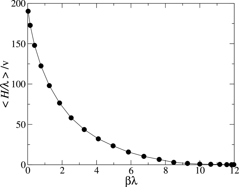
Figure 1: The average number of overlaps $\left\langle\frac{H}{\lambda}\right\rangle_{\lambda}$ , between colloidal particles and the walls per unit volume as a function of the height of the step potential for the pure colloidal system ($\eta_{p}^{r}=0$) with packing fraction $\eta_{c}=0.4$. For $\beta\lambda\geq 10$ the number of overlaps is zero within statistical fluctuations and the system behaves like the hard-sphere system. The line is a guide to the eye.

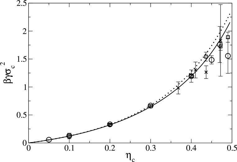
Figure 2: The reduced wall-fluid interfacial tension $\beta\gamma\sigma^{2}$ of hard spheres adsorbed at a hard wall as a function of the colloidal packing fraction $\eta_{c}$. We compare our simulation results (open circles) with Monte Carlo simulations M. Heni and H. Löwen (1999) (open squares) and Molecular Dynamics simulations J. R. Henderson and F. van Swol (1984) (crosses). The dotted line indicates the result from SPT and the solid line denotes the DFT result.

In this section we present the results on the interfacial tension of model colloid-polymer mixtures from simulation, SPT and DFT. We checked the simulation technique performing simulations for a system of pure hard spheres ($\eta_{p}^{r}=0$) and started by finding the optimal value for $\lambda_{\rm max}$, the maximum height of the potential (20). To this end, we computed the average number of overlaps $\left\langle\frac{H}{\lambda}\right\rangle_{\lambda}$ among particles and walls for different values of the potential height $\lambda$, with $H$ defined by the equation (20). The value of $\lambda_{\rm max}$ depends on the particle packing fraction. In Fig. 1 we plot the average number of overlaps between the colloidal particles and the walls for packing fraction $\eta_{c}=0.4$. For all values of $\beta\lambda\geq 10$, with $\beta=1/kT$ the inverse temperature, the average number of overlaps is zero within the statistical fluctuations. Smaller packing fractions require smaller values of $\beta\lambda_{\rm max}$. We checked the reliability of the approximation by computing the reduced wall-fluid interfacial tension $\beta\gamma_{\rm hs}\sigma_{c}^{2}$ (Fig. 2) and found that our simulation results are consistent with the results of Ref. M. Heni and H. Löwen (1999). At packing fraction $\eta_{c}\gtrsim 0.45$ the precision of the simulation is low but comparable with the simulation method of Heni and Löwen M. Heni and H. Löwen (1999) using the wall insertion method, and of Henderson and van Swol using the pressure tensor method J. R. Henderson and F. van Swol (1984). The agreement between simulation and density functional theory (DFT) R. Roth and S. Dietrich (2000); P. P. F. Wessels et al. (2004b) is remarkably good. The scaled particle theory (SPT) P. P. F. Wessels et al. (2004b) overestimates the wall-fluid tension at high density. This is due to the the inaccuracy of the SPT equation of state. Better results can be obtained combining the SPT equation for the interfacial tension and the Carnahan-Starling equation of state as explained in detail in Ref. M. Heni and H. Löwen (1999).

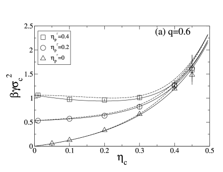
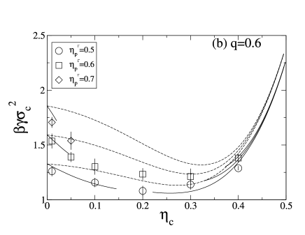
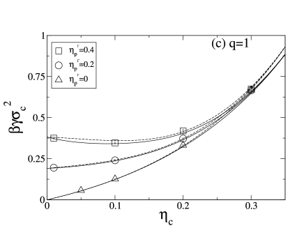
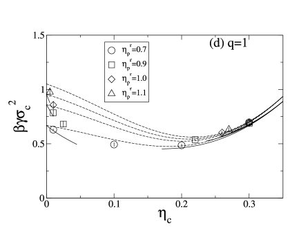
Figure 4: The wall-fluid interfacial tension of the model colloid-polymer mixture adsorbed against a hard wall. The symbols denote simulation results, dotted curves denote SPT results P. P. F. Wessels et al. (2004b), the solid curves denote DFT results P. P. F. Wessels et al. (2004b). a) Size ratio $q=0.6$ and $\eta_{p}^{r}=$0, 0.2, and 0.4; b) size ratio $q=0.6$ and $\eta_{p}^{r}=$0.5, 0.6, and 0.7; c) size ratio $q=1$ and $\eta_{p}^{r}=$0, 0.2, and 0.4; d) size ratio $q=1$ and $\eta_{p}^{r}=$0.7, 0.9, and 1.0.

We now determine the wall-fluid interfacial tension for AOV colloid-polymer mixtures of size ratio $q=0.6$ and $q=1$ for different values of the polymer reservoir packing fraction $\eta_{p}^{r}$ and of the colloid packing fraction $\eta_{c}$. The addition of nonadsorbing polymers to a colloidal suspension of hard-sphere can induce a phase separation. In Fig. 3 we show the bulk phase diagram for size ratio $q=1$ from previous simulations M. Dijkstra and R. van Roij (2002) in the ($\eta_{p}^{r}$,$\eta_{c}$) representation. For comparison, we also plot the phase diagram obtained from free volume theory, which is equivalent to our DFT phase diagram H. N. W. Lekkerkerker et al. (1992). At $\eta_{p}^{r}=0$ we find the freezing transition of the pure hard-sphere system with packing fractions $\eta_{c}^{f}\simeq 0.494$ and $\eta_{c}^{s}\simeq 0.545$ for the coexisting fluid and solid phase, respectively. The critical point is estimated to be at $\eta_{p,crit}^{r}=0.86$, while DFT, equivalent to the free-volume theory predicts $\eta_{p,crit}^{r}$= 0.638. For $\eta_{p}^{r}<eta_{p,crit}^{r}$, there is a stable fluid phase for $\eta_{c}<0.494$, a fluid-solid coexistence region for $0.494<\eta_{c}<0.545$, and a stable solid phase (fcc crystal) for $\eta_{c}>0.545$. For $\eta_{p}^{r}>\eta_{p,crit}^{r}$, a fluid-fluid coexistence region appears where the system demixes in a colloidal liquid phase, rich in colloids and poor in polymers, and a colloidal gas phase, that is poor in colloids and rich in polymers. The triple point, where the gas, the liquid, and the solid are in coexistence, is located at $\eta_{p,\rm triple}^{r}=6$. For $\eta_{p}^{r}>\eta_{p,triple}^{r}$, the fluid-fluid coexistence region disappears, and a wide crystal-fluid coexistence region appears. The overall phase diagram is analogous to that of a simple fluids upon identifying $\eta_{p}^{r}$ with the inverse temperature. Despite differences near the critical point, DFT and simulations results are in good agreement for state points at $\eta_{p}^{r}>1.5$. In Fig. 4a and Fig. 4c we show the wall-fluid tension for state points below the gas-liquid critical point for size ratio $q=0.6$ and $q=1$, respectively. For comparison, we also plot the results for pure hard spheres ($\eta_{p}^{r}=0$). The addition of non-adsorbing polymers to a suspension of hard-sphere colloids (i.e. increasing $\eta_{p}^{r}$) increases the wall-fluid interfacial tension. For $\eta_{c}=0$, the wall-tension is the work done to introduce an impenetrable wall in an ideal gas of polymers divided by the total area: $\beta\gamma(\eta_{c}=0)=\beta P^{id}\sigma_{p}/2$, where $\beta P^{id}=\rho_{p}^{r}$ is the bulk pressure of the ideal gas of polymer and $\sigma_{p}/2$ is the thickness of the depletion layer of the polymer at the wall. For small $\eta_{c}$, the slope of the tension is smaller than in the hard sphere case and for $\eta_{p}^{r}>=0.4$ it is negative. This is due to the attractive interaction that arises between the colloidal particles and the walls. For large $\eta_{c}$ the interfacial tension approaches that of pure hard spheres as at high colloid density the number of polymers in the mixture rapidly approaches zero. Simulations and DFT are in good agreement for all state points that we considered. The SPT predicts correctly the value at $\eta_{c}=0$, but it systematically overestimates the wall-fluid tensions for all values of $\eta_{c}>0$. One can show that the low $\eta_{c}$ expansion violates an exact wall sum rule Roth and Evans (2004). The deviation increases with increasing $\eta_{p}^{r}$. In Fig. 4b we show the results for size ratio $q=0.6$ for state points that are at higher $\eta_{p}^{r}$ than the DFT gas-liquid critical point. We did not calculate the binodal with computer simulation, but the system was still in the one phase region of the phase diagram for $\eta_{p}^{r}=0.5$ and 0.6. For comparison, we also plot the results from DFT and SPT. Note that DFT results are only shown in the stable gas and liquid regimes and are hence disconnected from each other, showing the biphasic region at intermediate $\eta_{c}$. In Fig. 4d we show the results for the size ratio $q=1$ for state points that are at higher $\eta_{p}^{r}$ than the DFT gas-liquid critical point. For small $\eta_{c}$ the SPT fails to reproduce the slope of the curves, due to the absence of colloid correlations (layering) near the hard-wall in SPT theory.

IV.2 Adsorption at a hard wall

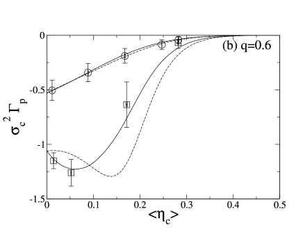
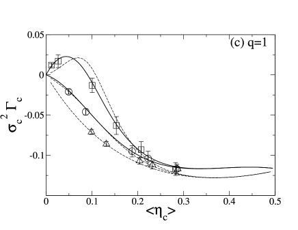
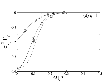
Figure 5: The adsorption $\Gamma\sigma_{c}^{2}$ of the colloid-polymer mixture at a hard wall as a function of the average colloid packing fraction $\langle\eta_{c}\rangle$. Simulation results for polymer reservoir packing fraction $\eta_{p}^{r}=0$ (open triangles), $\eta_{p}^{r}=0.2$ (open circles), and $\eta_{p}^{r}=0.4$ (open squares) are compared with results from DFT (solid lines) and SPT (dashed lines). The DFT results for $\eta_{p}^{r}=0$ are omitted for clarity. a) Colloid adsorption for size ratio $q$=0.6; b) Polymer adsorption for $q$=0.6; c) Colloid adsorption for $q$=1; d) Polymer adsorption for $q$=1.

In this section we present results on the adsorption of colloids and polymer at a hard-wall. We compare the simulation results with those from DFT and SPT Eqs. (9) and (10). In Figs. 5a and 5b, we show the results on the colloidal adsorption while in Figs. 5c and 5d, we show the results on polymer adsorption for size ratio $q$=0.6 and $q$=1, respectively. We notice that increasing the number of polymer in the system (i.e. increasing $\eta_{p}^{r}$) the adsorption of colloids increases; the colloids are attracted at the hard wall by the depletion interaction. As shown by the polymer adsorption the increase in number of colloidal particle at the walls is followed by a decrease of the number of adsorbed polymer while increasing the total number of polymers in the system. The agreement between simulations and DFT is good. This is not surprising since the DFT is known to provide an accurate description of the colloid-polymer mixture at a planar hard-wall J. M. Brader et al. (2003). The SPT equations reproduce the $\eta_{c}$=0 limit correctly. For $\eta_{c}\neq 0$ the essential features are reproduced but with low accuracy. We also note that the differences in SPT are larger for increasing polymer reservoir packing fraction and for size ratio $q$=0.6. The SPT performance is worse when the number of polymer in the mixture is relatively high compared to the number of colloids.

IV.3 Liquid-gas interfacial tension

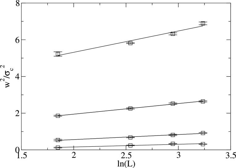
Figure 7: The squared width of the liquid-gas interface of the model colloid-polymer mixture with size ratio $q=1$ for polymer reservoir packing fractions $\eta_{p}^{r}=$0.95, 1.05, 1.4, 2 (from top to bottom), as a function of the logarithm of the lateral dimension of the interface. Symbols denote simulation results, lines indicate linear fits to the data.

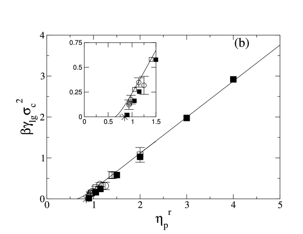
Figure 8: The reduced liquid-gas interfacial tension $\beta\gamma\sigma_{c}^{2}$ of the model colloid-polymer mixtures with size ratio $q=1$. Open squares denote simulation results from the capillary wave method. Filled squares indicate simulation results using the probability distribution method. Open circles refer to simulation results employing the difference $\gamma_{\rm wg}-\gamma_{\rm wl}$. The solid curves indicates the DFT results. The star indicate the position of the critical point, $\eta_{p}^{r}=0.86$, obtained from simulations. a) As a function of the difference in gas and liquid packing fractions $\eta_{c}^{l}-\eta_{c}^{g}$ at coexistence. b) As a function of the polymer reservoir packing fraction $\eta_{p}^{r}$, at coexistence. The inset shows the data close to the critical point on an enlarged scale.

In this section we present results on the liquid-gas interfacial tension of AOV colloid-polymer mixtures of size ratio $q$=1, using three independent simulation techniques explained above. First we use the scaling of the interfacial width. The Fig. 6 shows typical snapshots of the liquid-gas interface for $\eta_{p}^{r}=$0.95, 1.05, 1.4, and 2.0. One observes clearly that the difference in densities of the two coexisting phases increases with increasing $\eta_{p}^{r}$. Moreover, the liquid-gas interface becomes sharper upon increasing $\eta_{p}^{r}$. The interfacial order parameter $\Psi(z)$ is determined and fitted to an error function to extract the interfacial width. In Fig. 7 we plot the square of the interfacial width as a function of the logarithm of the lateral dimension $L$. Employing a linear fit to our data and using Eq. (44), we determine $\gamma_{{\rm lg}}$. In Fig. 8a and Fig. 8b we plot the liquid-gas interfacial tension as a function of $\eta_{c}^{l}-\eta_{c}^{g}$ and $\eta_{p}^{r}$ respectively. We determine the colloid densities $\eta_{c}^{l}$ and $\eta_{c}^{g}$ at coexistence from the measured density profile $\rho_{c}(z)$.

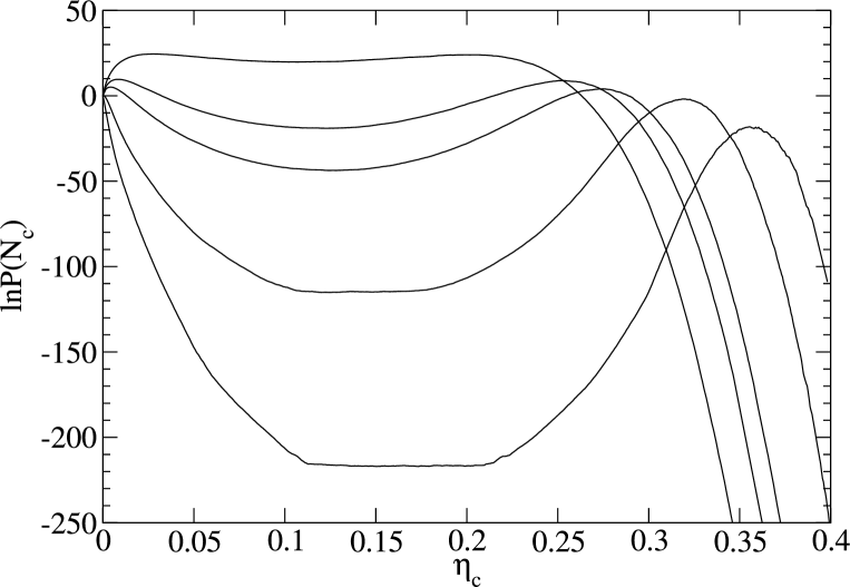
Figure 9: Logarithm of the probability $P(N_{c})$ (not normalized, as P(0) is taken to be 1) of finding $N_{c}$ colloids with diameter $\sigma_{c}$ for a colloid-polymer mixture with size ratio $q=1$ in a cubic box with volume $V=1000\sigma_{c}^{3}$ at varying polymer reservoir packing fraction $\eta_{p}^{r}=$0.9, 1.05, 1.15, 1.5, and 2 (from top to bottom), as a function of $\eta_{c}$. All statepoints are at coexistence.

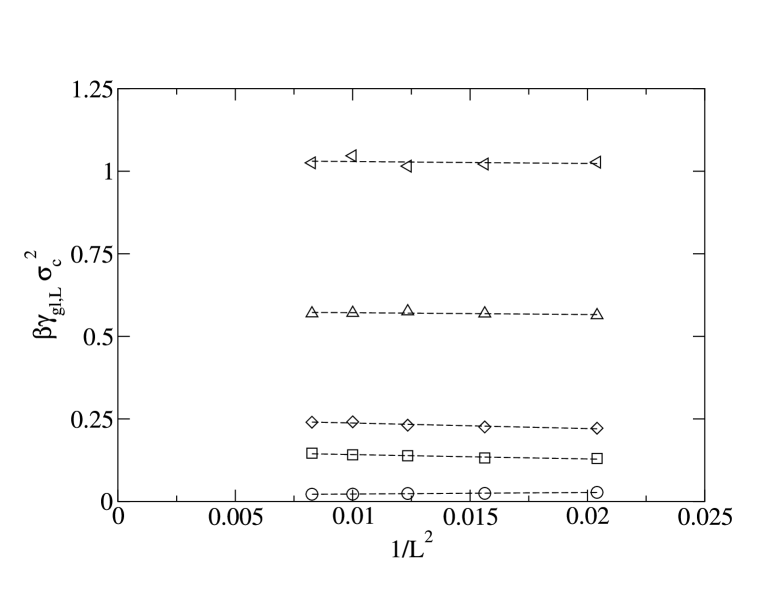
Figure 10: The system size dependence of the (scaled) liquid-gas interfacial tension $\beta\gamma_{{\rm lg},L}\sigma_{c}^{2}$ of a colloid-polymer mixture with size ratio $q=\sigma_{p}/\sigma_{c}=1$ in a cubic box with volume $V=L^{3}\sigma_{c}^{3}$ at varying polymer reservoir packing fraction $\eta_{p}^{r}=0.9,1.05,1.15,1.5,$ and 2.0 (from bottom to top). The dashed lines are least-squares linear fits.

Than in the second method we determined the probability distributions $P(N_{c})|_{z_{c},\eta_{p}^{r}}$ for $\eta_{p}^{r}=$0.9, 1.05, 1.15, 1.5, 2.0, 3.0, and 4.0 in a cubic simulation box of length $L=7,8,9,10,$ and 11. We show the probability distribution for box length $L=10$ for varying $\eta_{p}^{r}$ in Fig. 9. We observe clearly that the density jump at coexistence and $\gamma_{{\rm lg},L}$, i.e., the difference of the maxima and minimum, increases with $\eta_{p}^{r}$. We determined $\gamma_{{\rm lg}}$ for an infinite system by plotting $\gamma_{{\rm lg},l}$ as a function of $1/L^{2}$ in Fig. 10 and extrapolating, $L\rightarrow\infty$, according to Eq. (51). Again, we plot the liquid-gas interfacial tension as a function of $\eta_{c}^{l}-\eta_{c}^{g}$ and $\eta_{p}^{r}$ in Figs. 8a and Fig. 8b, respectively. We determined $\eta_{c}^{g}$ and $\eta_{c}^{l}$ at coexistence from

$$\eta_{c}^{g}=\frac{2\pi\sigma_{c}^{3}}{6}\int_{0}^{\langle N_{c}\rangle}N_{c}P(N_{c})|_{z_{c}^{\prime},\eta_{p}^{r}}dN_{c}\hskip 28.45274pt\eta_{c}^{l}=\frac{2\pi\sigma_{c}^{3}}{6}\int_{\langle N_{c}\rangle}^{\infty}N_{c}P(N_{c})|_{z_{c}^{\prime},\eta_{p}^{r}}dN_{c}$$ (53)

where the factor 2 arises from the normalization (47). Finally, we also employed Young’s equation to obtain an estimate for $\gamma_{{\rm lg}}$. Dijkstra et al. M. Dijkstra and R. van Roij (2002) studied the wetting behavior of AOV model colloid-polymer mixtures using computer simulations. From measuring adsorption isotherms they concluded that the colloidal liquid phase wets the wall completely upon approaching the gas branch of the gas-liquid bulk binodal for values of $\eta_{p}^{r}<1.05$. In this region the contact angle vanishes and $\gamma_{{\rm lg}}=(\gamma_{\rm wg}-\gamma_{\rm wl})$, where $\gamma_{\rm wg}$ and $\gamma_{\rm wl}$ are wall-fluid tensions $\gamma_{\rm wf}$ computed at liquid-gas coexistence. We hence carried out simulations of the wall-fluid tension for statepoints at coexistence below the wetting transition point: $\eta_{p}^{r}=0.935$, and $0.977$ and also slightly above the wetting transition point: $\eta_{p}^{r}=1.14$ and $1.25$. The coexisting densities were previously determined in Gibbs ensemble simulations (see Fig. 3). We stress that the results obtained on the basis of Young’s equation should be taken with great care, as the wall-gas tension in our simulations were obtained from a gas phase in contact with a planar hard wall, which is a metastable state with respect to the equilibrium state of a macroscopic wetting layer adsorbed at the gas-wall interface.

However, DFT results show that the contact angle differs only less than few a percent when the metastable gas-wall density profile is employed instead of the stable density profile that includes the wetting layer. In Fig. 8a and Fig. 8b we plot the difference $\gamma_{\rm wg}-\gamma_{\rm wl}$ for $\eta_{p}^{r}=0.935,0.977,1.14,$ and $1.25$. Comparing the results obtained for $\gamma_{{\rm lg}}$ from the three different routes, we find good agreement. The agreement with DFT results is good for high values of $\eta_{c}^{l}-\eta_{c}^{g}$ and $\eta_{p}^{r}$, but deviates close to the critical point, as might be expected. Similar deviations were found for $\gamma_{{\rm lg}}$, by Vink et al. using the probability distribution method in simulation of the full mixture for size ratio $q=0.8$ R. L. C. Vink and J. Horbach (2004b).

V Conclusions

In conclusion we investigated the wall-fluid tension of the AOV model colloid-polymer mixtures of size ratio $q=0.6$ and $q=1$ using Monte Carlo computer simulations. We used a thermodynamic integration method and a shoulder potential approximation for the hard-core potentials to determine the free energy of the bulk system and the inhomogeneous system. The wall-fluid interfacial tension is the surface excess free energy per unit area, and is in good agreement with the DFT results. The SPT wall-fluid interfacial tension is in overall agreement with simulations, but the comparison is worse for increasing polymer reservoir packing fraction. We also investigated the colloid and polymer adsorption of the colloid-polymer mixture at a planar hard wall and we found good agreement with DFT results. We derived a SPT expression for the adsorption of colloid polymer mixtures at a hard wall. The expression reproduce the essential features of the adsorption, but with low accuracy. In addition, we studied the liquid-gas interfacial tension of the AOV model colloid-polymer mixtures of size ratio $q=1$ using i) the dependence of the interfacial width on the logarithm of the lateral size of the simulation box as predicted by the capillary wave theory, ii) the probability distribution method, and iii) Young’s equation in the complete wetting regime. We find remarkably good agreement between the different sets of results. Moreover, as we used the effective one-component simulations in the probability distribution method, we were able to investigate the interfacial tension for high $\eta_{p}^{r}$. As the bulk binodal from DFT, equivalent to that of free-volume theory H. N. W. Lekkerkerker et al. (1992), agrees well with the simulation results for $\eta_{p}^{r}>1.5$, one might expect a similar agreement for the interfacial tension. We found that our simulation results for $\gamma_{{\rm lg}}$ approaches the DFT results upon increasing $\eta_{p}^{r}$ and agree well with the DFT results only for $\eta_{p}^{r}>3$. Close to the critical point, deviations are found between the simulation and DFT results as expected due to the shift in critical point.

The good agreement of our simulation results for wall-fluid and fluid-fluid interfacial tensions with those of the DFT hint at a reliable description of the magnitude of contact angle of the colloidal liquid-gas interface and a hard wall P. P. F. Wessels et al. (2004a). Nevertheless, carrying out detailed simulations at bulk coexistence in the (numerically very demanding) partial wetting regime of large $\eta_{p}^{r}$ is an interesting issue for future work, in particular in light of the fact that the contact angle can be measured in a direct (though not easy) way in experiments D. G. A. L. Aarts and H. N. W. Lekkerkerker (2004); W. K. Wijting et al. (2003b, a). Furthermore our thermodynamic integration technique is well suited to determine the free energy of confined crystals and hence to predict the full phase behavior of confined colloid-polymer mixtures; work along these lines is in progress. Finally we mention that interfacial properties at curved substrates have attracted recent interest Evans et al. (2003, 2004); colloid-polymer mixtures are well-suited to investigate such situations D. G. A. L. Aarts and H. N. W. Lekkerkerker (2004).

Figure 3: Phase diagram of the AOV model for size ratio $q=1$ as obtained from simulations, taken from Refs. M. Dijkstra and R. van Roij (2002) (symbols), and free volume theory H. N. W. Lekkerkerker et al. (1992) (dashed line) as a function of the colloid packing fraction $\eta_{c}$ and the polymer reservoir packing fraction $\eta_{p}^{r}$. F and S denote the stable fluid and solid (fcc) phase. F+S and F+F denote, respectively, the stable fluid-fluid, and fluid-solid coexistence region.