Cross-dimensional relaxation in Bose-Fermi mixtures

Abstract

We consider the equilibration rate for fermions in Bose-Fermi mixtures undergoing cross-dimensional rethermalization. Classical Monte Carlo simulations of the relaxation process are performed over a wide range of parameters, focusing on the effects of the mass difference between species and the degree of initial departure from equilibrium. A simple analysis based on Enskog’s equation is developed and shown to be accurate over a variety of different parameter regimes. This allows predictions for mixtures of commonly used alkali atoms.

I Introduction

In the study of ultracold dilute atomic gases, the interparticle interactions are characterized by the $s$-wave scattering length $a$. Because of the low temperatures achieved, and the lack of long range or anisotropic interactions, the value of $a$ determines a wide variety of equilibrium and dynamical properties of quantum degenerate gases. Furthermore the parameter $a$ can be tuned in many systems, from $-\infty$ to $\infty$ by means of Feshbach resonances FRtheory , allowing the experimenter access to any desired interaction strength. This potential for real-time control over interactions is a unique feature of ultracold gas experiments. Additionally the efficiency of evaporative cooling relies on a large elastic collision rate, which is proportional to $a^{2}$. For these reasons, the ability to accurately determine the scattering properties of dilute ultracold gases becomes essential for quantum gas experiments.

In their pioneering work with ultracold ¹³³Cs atoms, Monroe and co-workers showed that a relatively simple rethermalization measurement starting with a non-equilibrium gas could provide a determination of the elastic collision cross-section Mon93 , which is equal to $8\pi a^{2}$ for identical non-condensed bosons. The rethermalization rate for a gas in the so-called collisionless regime (defined by a collision rate per particle much lower than the harmonic frequencies of the trapping potential), was measured by selectively removing energy from the gas in one spatial dimension and watching the subsequent cross-dimensional rethermalization. The relaxation in such experiments is driven by elastic collisions, and an analysis based on Enskog’s equation shows that the rate of relaxation is proportional to the mean rate of collisions Rob01 ; Rei65 ,

$$\Gamma_{\rm relax}=\frac{1}{\alpha}\,\langle n\rangle\,\sigma\,\langle v_{\rm rel}\,\rangle\quad,$$ (1)

where $n$ is the number density of the gas, $\sigma$ is the elastic collision cross-section, and $v_{\rm rel}$ is the relative collision speed; brackets $\langle\cdot\rangle$ denote a thermal average, and we have used the assumptions of energy-independent $s$-wave collisions and Boltzmann statistics to write the mean collision rate $\langle\,\Gamma_{\rm coll}\,\rangle=\langle n\,\sigma\,v_{\rm rel}\rangle=\langle n\rangle\,\sigma\,\langle v_{\rm rel}\rangle$. The constant of proportionality $\alpha$, defined as the ratio of collision and relaxation rates, reflects the mean number of collisions per particle required for rethermalization. A variety of numerical and analytical studies have found that $\alpha$ is between $2.5$ and $2.7$ Mon93 ; Rob01 ; Wu96 ; Kav98 ; DeM99 .

We have recently extended the method of cross-dimensional relaxation to probe the $s$-wave scattering length $a_{BF}$ between bosonic and fermionic atoms in a Bose-Fermi mixture Gol04 . In that work, we compared single-species boson rethermalization to relaxation of fermions in the presence of bosons in order to eliminate the systematic calibration error associated with atom number that typically dominates cross-dimensional rethermalization measurements. Since collisions between spin-polarized ultracold fermions are forbidden by the Pauli exclusion principle DeM99 , their rethermalization proceeds only through collisions with the bosons. The collision rate per fermion in the mixture therefore depends only on the number of bosons, allowing us to write the mean relaxation rate per fermion in analogy with the single-species case,

$$\Gamma_{F}=\frac{1}{\beta}\,\langle n_{B}\rangle\,\sigma_{BF}\,\langle v_{BF}\rangle\quad.$$ (2)

Here $\langle n_{B}\rangle$ is the equilibrium density of the bosons, averaged over the fermion distribution, $\sigma_{BF}$ is the boson-fermion elastic cross section, and $\langle v_{BF}\rangle=(8\,k_{B}T/\pi\mu)^{1/2}$ is the thermally averaged relative collision speed between bosons and fermions with reduced mass $\mu=m_{F}\,m_{B}/(m_{F}+m_{B})$ and temperature $T$ ($k_{B}$ is Boltzmann’s constant). The cross-section is related to the interspecies scattering length by $\sigma_{BF}=4\pi a_{BF}^{2}$. The constant of proportionality $\beta$ reflects the mean number of collisions per fermion needed for rethermalization. Knowledge of $\alpha$ and $\beta$ was essential in achieving both the accuracy and precision of the measurement in Ref. Gol04 .

In this work, we study the general dependence of $\beta$ on the masses of the fermions and bosons by means of detailed classical Monte Carlo simulations of the relaxation process. We additionally address the effect due to the finite initial departure from equilibrium. Understanding this effect is a necessary component of the analysis of both the simulations and the measurements, where a larger initial perturbation improves the signal-to-noise ratio. We further develop a classical kinetic model based on Enskog’s equation for the case of Bose-Fermi mixtures that reproduces the behavior of the simulations. The analysis and simulations show the following: (i) Equation (2) is valid for a wide range of parameters relevant to current experiments, (ii) the difference in mass between the bosons and fermions can lead to a $\sim 5$ times difference in $\beta$ between light and heavy fermions in mixtures of experimental interest, and (iii) the size of the initial perturbation must be taken into account to fully understand the results.

The remainder of the paper is organized as follows. In Sec. II we describe the details of the Monte Carlo simulations and use the simulations to verify the validity of Eq.(2). In Sec. III the mass dependence of the relaxation is investigated using the simulations and compared to a classical kinetic theory that is developed in some detail. It is shown that the model reproduces the behavior of the simulations over a wide range of masses. In Sec. IV the importance of the size of the initial perturbation is addressed. Finally, we conclude in Sec. V with a discussion of possible extensions of the model and further applications of the Monte Carlo simulations.

II Monte Carlo Simulation

Implicit in the definition of $\beta$ in Eq.(2) are the assumptions that the energy anisotropy undergoes exponential decay Wu96 and that $\beta$ depends only on intrinsic properties of the particles under study, such as the mass and quantum statistics, and not the bulk properties of the gases, such as the temperature or atom numbers (assuming one remains always in the collisionless regime). These assumptions were verified by running Monte Carlo simulations of the relaxation.

In the experiment considered here, we start with a Bose-Fermi mixture that is in thermal equilibrium in a cylindrically symmetric harmonic trap and increase the radial trapping frequency by a factor of $\Omega$ to produce the initial energy anisotropy in the system; the axial frequency is unchanged. The change in trap strength is performed slowly with respect to the radial trap periods but quickly compared to the thermal relaxation time. The increase in radial energies $E_{x,y}$ is then the same for each species and is equal to the fractional increase in the trapping frequencies. Therefore the ratio of radial and axial energies immediately before rethermalization is simply

$$\left.\frac{E_{x,y}}{E_{z}}\right|_{t=0}=\Omega\quad.$$

Note that for gases prepared in this manner, $E_{x}\approx E_{y}$ at all times. Since the gases rethermalize together, they reach the same final temperature. In the classical gas limit, the final temperature is given by $(T_{\infty}/T_{0})=(1+2\,\Omega)/3$, where $T_{0}$ is the temperature before compression. It is important to note that for this type of rethermalization, there is no net transfer of energy between species during the relaxation process; this fact is essential for the validity of Eq.(2).

An outline of the Monte Carlo simulation is as follows. An ensemble consisting of $N_{B}$ bosons and $N_{F}$ fermions is prepared in a cylindrically symmetric harmonic trapping potential. The ensemble is initialized by assigning a random position and velocity vector to each particle from separable Gaussian distributions. The distributions are scaled such that there is a factor of $\Omega$ imbalance between the mean energies per particle (both kinetic and potential) in the transverse ($x,y$) and axial ($z$) dimensions. The initial energy in a given dimension, however, is the same for both species. The positions and velocities are evolved for some small time step $\Delta t$ according to Newton’s laws in the trap, and then collisions are considered.

Only boson-boson and boson-fermion collisions are allowed, in accordance with the Pauli exclusion principle for a system with spin-polarized fermions. If two particles are found within a critical distance $r_{c}$ of each other, the pair is given a chance to collide. The collision probability is given by $P_{\rm coll}=\sigma_{kl}\,v_{\rm rel}\,\Delta t/{\mathcal{V}}_{c}$, where $\sigma_{kl}$ is the collision cross section between particles $k$ and $l$, $v_{\rm rel}=|\vec{v}_{k}-\vec{v}_{l}|$ is the relative collision speed, and ${\mathcal{V}}_{c}=4\pi\,r_{c}^{3}/3$ is the volume of the sphere containing the colliding atoms. If $P_{\rm coll}$ is greater than a uniformly distributed random number between zero and one, then the relative velocity vector is rotated into a random direction (conserving the total momentum and energy) to represent an $s$-wave collision. Finally, after all possible collision pairs have been considered, the mean energies of each species in each of the three cartesian directions are recorded, and a new time step proceeds.

In agreement with Ref.Gue99 we find it essential for obtaining robust results to set $\Delta t$ and $r_{c}$ such that the ensemble average collision probability $\langle P_{\rm coll}\rangle$ and occupation of the fictional spheres surrounding the atoms are both well below $10\%$. Typical values for our simulations are $\Delta t\sim 10^{-3}$ to $10^{-2}$ times the collision time $\langle n\,\sigma\,v_{\rm rel}\rangle^{-1}$, and $r_{c}\sim 10^{-3}$ to $10^{-2}$ times the root-mean-squared (rms) cloud radius. Since the motion between collisions is known analytically, it is not necessary to keep $\Delta t$ small compared to the trap period. Finally, we note that we have not observed any double-counting of collisions in consecutive time steps. This is because our time step $\Delta t$ typically satisfies $v\,\Delta t\gg r_{c}$, where $v$ is the characteristic speed of the particles.

A typical relaxation curve obtained from the simulation is shown in Fig. 1. The relaxation rate $\Gamma_{F}$ of the energy anisotropy of the fermions is determined by fitting the ratio of radial and axial energies to the ratio of decaying exponentials,

$$\frac{1}{2}\,\frac{E_{x}+E_{y}}{E_{z}}=\frac{1+\varepsilon\exp(-\Gamma_{F}\,t)}{1-2\,\varepsilon\exp(-\Gamma_{F}\,t)}\quad.$$

Here, $E_{i}$ is the mean total energy per particle of the fermions in the $i^{\rm th}$ direction, and $\varepsilon=(\Omega-1)/(1+2\Omega)$ characterizes the amount of initial perturbation from equilibrium.

Figure 1: Typical Monte Carlo simulation of cross-dimensional relaxation of fermions in the presence of bosons. The mean energy per fermion $E_{i}$ in each direction is shown versus time during the equilibration process. The curves represent $5\times 10^{4}$ fermions in the presence of $5\times 10^{4}$ bosons. The calculation used ⁴⁰K (⁸⁷Rb) as the fermion (boson), and the trapping frequencies, temperature, and initial perturbation were taken from the experiment in Ref. Gol04 . A cross-species scattering length of $|a_{BF}|=235\,a_{0}$, with $a_{0}$ the Bohr radius, was assumed. The calculated mean time between collisions is $0.23$ s.

The validity of Eq.(2) was tested by running Monte Carlo simulations with varying temperatures, numbers of atoms, trapping frequencies, and interspecies cross-sections $\sigma_{BF}$. As an example, the dependence of $\Gamma_{F}$ on the number of bosons ($N_{B}$) and fermions ($N_{F}$) in the mixture is shown in Fig. 2. The results show that $\Gamma_{F}$ varies linearly with $N_{B}$, while it is constant when changing $N_{F}$ over the same range. Although these simulations assumed $|a_{BF}|=235\,a_{0}$ and $a_{BB}=98.98\,a_{0}$ Kem02 , results similar to those in Fig. 2 were obtained for $a_{BF}=50\,a_{0}$, corresponding to a ratio of cross-sections $(\sigma_{BB}/\sigma_{BF})=0.35$ and $7.8$, respectively.

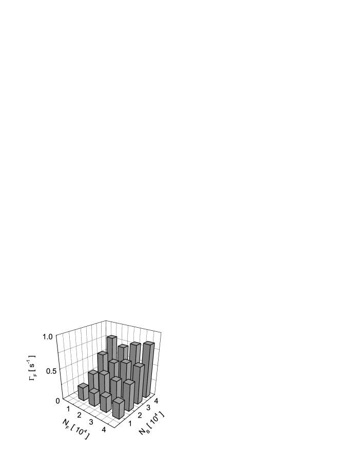
Figure 2: Fermion rethermalization rate $\Gamma_{F}$ as a function of $N_{B}$ and $N_{F}$. These calculations used the parameters from the ⁸⁷Rb-⁴⁰K experiment in Ref.Gol04 , with $|a_{BF}|=235\,a_{0}$.

III Mass Dependence — Classical Kinetic Model

The Monte Carlo simulation is a powerful tool for analyzing the behavior of relaxing Bose-Fermi mixtures, but it requires a considerable amount of computing resources. For example, one of our simulations using $10^{4}$ fermions and $10^{4}$ bosons with $10^{4}$ time steps took over 8 hours on a Unix system with a $2.4$ GHz processor and 4 GB of RAM. The computation time, which is dominated by the pairwise search for collision partners, scales roughly as the product of the number of time steps and $N_{B}\,(N_{F}+N_{B}/2)$, so that simulations become impractical for $N\gtrsim 10^{5}$. Furthermore, it is desirable to build up a physical picture of the relaxation that is not provided by the simulations. For these reasons, we now consider an analytic model of the rethermalization.

One new degree of freedom for two-species rethermalization is the appearance of a second mass. In order to see how the number of collisions per fermion needed for rethermalization depends on the masses of the particles involved, we first consider the two limiting cases of very light and very heavy fermions. Recall that energy is redistributed by means of $s$-wave collisions, which randomize the relative velocities of the colliding particles. For very light fermions, a single collision should be nearly enough to redistribute the energy. If the fermions are far heavier than the bosons, however, it should take many collision times to redistribute the energy, since a single collision has little effect on the motion of the heavy particle. We therefore expect the number of collisions needed for equilibration to be a monotonically increasing function of the normalized fermion mass $\eta=m_{F}/(m_{F}+m_{B})$. Note that this is in contrast to the behavior of two gases initially at different (isotropic) temperatures and subsequently brought into contact for rethermalization. In the latter case, one expects $\beta^{-1}\propto 4\,\eta\,(1-\eta)$ Mos01 , which is most efficient for $\eta=1/2$. The results of our Monte Carlo simulations is shown as the solid points in Fig. 3. As expected, $\beta$ increases smoothly with the fermion mass. The open points and solid lines are predictions from a simple kinetic model, which we now discuss in detail.

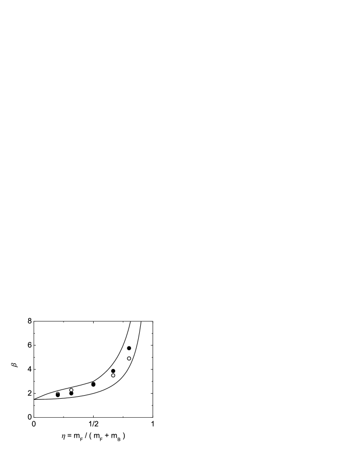
Figure 3: Dependence of the mean number of collisions per fermion needed for rethermalization on the normalized fermion mass. Solid points ($\bullet$) are the results of the Monte Carlo simulations, and open points ($\circ$) are from exponential fits to our model from Eq.(8). The solid lines are the bounding predictions from the classical kinetic model. The number of atoms is $N_{B}=N_{F}=10^{4}$, the initial perturbation is $\Omega=1.64$, and the ratio of cross sections is $(\sigma_{BB}/\sigma_{BF})=0.35$.

Our analysis of the rethermalization process is based on Enskog’s equation, which is equivalent to the Boltzmann transport equation Rei65 . This treatment gives the rate of change of the ensemble average of any function of the boson and fermion positions and velocities, usually denoted $\chi(\vec{x}_{B},\vec{v}_{B};\vec{x}_{F},\vec{v}_{F})$, by

$$\dot{\langle\,\chi\,\rangle}=\sigma\,\langle\,n\,v_{\rm rel}\,\Delta\chi\,\rangle\quad,$$ (3)

where we have again used the assumption of energy-independent $s$-wave scattering to separate the collision cross-section $\sigma$ from the ensemble average. The quantity $\Delta\chi$ is just the change in $\chi$ due to a single collision. Here we consider

$$\chi_{1}\equiv E_{1x}-E_{1z}\quad,$$ (4)

where we are focusing for now on generic particles of type 1 colliding with particles of type 2. The energy $E_{1i}$ denotes the total (kinetic plus potential) energy of type-1 atoms in the $i^{\rm th}$ direction. Note that our current interest in $\chi_{1}$ implies the ensemble average in Eq.(3) is taken only over the distribution function for type-1 atoms. Based on the results of Fig. 2, we can assume equal numbers of atoms $N_{1}=N_{2}$ without loss of generality.

Immediately after a collision, only the kinetic energy (KE) has changed, so that

$$\Delta\chi_{1} = \Delta({\rm KE}_{1x}-{\rm KE}_{1z})$$

$$= \frac{1}{2}\,m_{1}\,\Delta(v_{1x}^{2}-v_{1z}^{2})\quad.$$

Since $\Delta\chi_{1}$ has no position dependence, we can remove the type-2 particle density $n_{2}$ from the average, yielding

$$\dot{\langle\,\chi_{1}\,\rangle}=\frac{1}{2}\,m_{1}\,\langle\,n_{2}\,\rangle\,\sigma_{12}\,\langle\,v_{\rm rel}\,\Delta(v_{1x}^{2}-v_{1z}^{2})\,\rangle\quad.$$

We define CM and relative velocities in the usual manner,

$$\vec{V}_{\rm CM} = \frac{m_{1}\vec{v}_{1}+m_{2}\,\vec{v}_{2}}{m_{1}+m_{2}}$$

$$\vec{v}_{\rm rel} = \vec{v}_{1}-\vec{v}_{2}\quad,$$ (5)

which gives

$$v_{1x}^{2}-v_{1z}^{2} = \left(V_{{\rm CM}x}^{2}-V_{{\rm CM}z}^{2}\right)$$

$$+\left(\frac{m_{2}}{m_{1}+m_{2}}\right)^{2}\left(v_{{\rm rel}x}^{2}-v_{{\rm rel}z}^{2}\right)$$

$$+\,2\,\frac{m_{2}}{m_{1}+m_{2}}\left(V_{{\rm CM}x}\,v_{{\rm rel}x}-V_{{\rm CM}z}\,v_{{\rm rel}z}\right)\quad.$$

Since the collision leaves $\vec{V}_{\rm CM}$ and $|\vec{v}_{\rm rel}|$ unchanged, but randomly rotates the direction of $\vec{v}_{\rm rel}$, we are left with

$$\dot{\langle\,\chi_{1}\,\rangle} = -\frac{1}{2}\,\frac{m_{1}\,m_{2}}{(m_{1}+m_{2})}\,\langle\,n_{2}\,\rangle\,\sigma_{12}$$

$$\times\,\left\langle v_{\rm rel}\left[\,\frac{m_{2}}{m_{1}+m_{2}}\,\left(v_{{\rm rel}x}^{2}-v_{{\rm rel}z}^{2}\right)\right.\right.$$

$$\left.\left.+\frac{}{}\,2\left(V_{{\rm CM}x}\,v_{{\rm rel}x}-V_{{\rm CM}z}\,v_{{\rm rel}z}\right)\,\right]\,\right\rangle\quad.$$

Here we need only consider the quantities immediately before the collision since there is no preferred direction for $\vec{v}_{\rm rel}$ after the collision. Note also that $\langle\,V_{{\rm CM}i}\,v_{{\rm rel}i}\,\rangle\neq 0$ for a gas with a cross-dimensional energy anisotropy.

Calculating these ensemble averages for arbitrary masses and energy anisotropies (which are in general different between species) is non-trivial, but some simple approximations may be used. For the first term it is easy to show that for Boltzmann distributions in equilibrium one has

$$\langle\,v_{\rm rel}\,v_{{\rm rel}x}^{2}\,\rangle=\frac{4}{3}\,\langle\,v_{\rm rel}\,\rangle\,\langle\,v_{{\rm rel}x}^{2}\,\rangle\quad.$$ (6)

For cross-terms of the form $\langle\,V_{{\rm CM}x}\,v_{{\rm rel}x}\,\rangle$, which vanish under equilibrium conditions, one can still consider the limit of small deviation from thermal equilibrium. In this case we obtain, similar to the above result,

$$\langle\,v_{\rm rel}\,V_{{\rm CM}x}\,v_{{\rm rel}x}\,\rangle = \frac{4}{3}\,\left\langle\,v_{\rm rel}\,\rangle\,\langle\,V_{{\rm CM}x}\,v_{{\rm rel}x}\,\right\rangle\quad.$$

We verified by analytic means and with Monte Carlo integrations of Gaussian distributions that these approximations are reasonable for small anisotropies.

Combining these results gives

$$\dot{\langle\,\chi_{1}\,\rangle} = -\frac{2}{3}\,\langle\,\Gamma_{12}\,\rangle\,\frac{m_{1}\,m_{2}}{m_{1}+m_{2}}\,\left\langle\,\frac{m_{2}}{m_{1}+m_{2}}\,\left(v_{{\rm rel}x}^{2}-v_{{\rm rel}z}^{2}\right)\right.$$

$$\left.+\frac{}{}\,2\left(V_{{\rm CM}x}\,v_{{\rm rel}x}-V_{{\rm CM}z}\,v_{{\rm rel}z}\right)\,\right\rangle\quad.$$

The collision rate $\Gamma_{12}$ describes the rate per type-1 particle of collisions with particles of type 2. If we finally substitute back with $v_{1}$ and $v_{2}$, and use $\langle\,v_{1i}\,v_{2i}\,\rangle=0$, we obtain

$$\dot{\chi}_{1}=-\frac{2}{3}\,\Gamma_{12}\,\frac{m_{2}}{(m_{1}+m_{2})^{2}}\,\left[\,(2\,m_{1}+m_{2})\,\chi_{1}-m_{1}\,\chi_{2}\,\right]$$ (7)

where we have dropped the angle brackets now for simplicity. Note that we have used the fact that the mean kinetic and potential energies in a given direction are equal in the collisionless regime.

For concreteness, we now associate the type-1 particles with the fermions and type-2 particles with the bosons. The time-dependence of $\chi_{2}$, defined in analogy with Eq.(4), is obtained by swapping $1\leftrightarrow 2$ in Eq.(7) and adding a term describing the effect of boson-boson collisions. This term was calculated from Enskog’s equation in Ref.Rob01 , giving $\alpha=5/2$ in the limit of small energy anisotropy. This yields the final result,

$$\frac{d}{d\,\tau}\;\chi_{1} = -\frac{2}{3}\,\frac{m_{2}}{(m_{1}+m_{2})^{2}}\,\left[\,(2\,m_{1}+m_{2})\,\chi_{1}-m_{1}\,\chi_{2}\,\right]$$

$$\frac{d}{d\,\tau}\;\chi_{2} = -\frac{2}{3}\,\frac{m_{1}}{(m_{1}+m_{2})^{2}}\,\left[\,(2\,m_{2}+m_{1})\,\chi_{2}-m_{2}\,\chi_{1}\,\right]$$ (8)

$$-\frac{\gamma}{\alpha}\,\chi_{2}\quad,$$

where we have introduced the dimensionless time $\tau=\Gamma_{12}\,t$ and the ratio of collision rates $\gamma=\Gamma_{22}/\Gamma_{12}$ (note that $\Gamma_{12}=\Gamma_{21}$ for Boltzmann distributions with $N_{1}=N_{2}$ under conditions of thermal equilibrium).

Equation (8) is the main result of our analysis. The results of exponential fits to the time-evolution of Eq.(8) are shown as the open points in Fig. 3. The slight overestimation (underestimation) for light (heavy) fermions is a result of our approximation in Eq.(6). Although the full solution to Eq.(8) requires prior knowledge of the inter-species cross-section $\sigma_{12}$ (through $\gamma$), we now show that the solutions in the limits $\gamma=0$ and $\gamma\to\infty$ provide tight bounds on $\beta$. These two limits are shown as the solid lines in Fig. 3.

In the case $\gamma\gg 1$, where boson-boson collisions occur much more frequently than boson-fermion collisions, we can assume the energy of the bosons is always isotropic and take $\chi_{2}=0$ for all times. In this limit, Eq.(8) is easily solved, giving

$$\chi_{1}(\tau)=\chi_{1}(0)\exp\left(-\frac{\tau}{\beta_{l}}\right)\quad.$$

with $\beta_{l}$ given by

$$\beta_{l}=\frac{3}{2}\,\frac{1}{1-\eta^{2}}\quad,$$ (9)

The solution to Eq.(8) in the limit $\gamma\to 0$ does not correspond exactly to a simple exponential but rather to the sum (or difference) of decaying exponentials. Heavy fermions ($\eta>1/2$) rethermalize slowly at first and then more quickly as the energy of the bosons becomes isotropic. In this case, we obtain an upper limit on $\beta$ by simply taking the small-$\tau$ expansion of the solution to Eq.(8), giving $\beta_{u}=(3/2)(1-\eta)^{-1}$. For light fermions ($\eta<1/2$), we obtain $\beta_{u}$ by fitting the solution of Eq.(8) to the simple exponential decay minimizing the chi-squared error. Our values for $\beta_{u}$ and $\beta_{l}$ are shown in Fig. 3 as the upper and lower solid lines, respectively. The results from the Monte Carlo simulations fall within these limits as expected. Simulations with different atom numbers and cross-sections gave similar results.

IV Discussion

Before proceeding, we first consider the effect of the finite size of the initial perturbation. Our analysis has so far been limited to the case of arbitrarily small initial anisotropies. As discussed in the introduction, however, experiments (as well as Monte Carlo simulations) require large anisotropies for good signal-to-noise ratios. It was noted in Ref.Wu96 that the mean collision rate per particle $\langle\,\Gamma_{\rm coll}\,\rangle=\langle n\rangle\,\sigma\,\langle v_{\rm rel}\rangle$ actually changes during the relaxation process, because of the redistribution of energy. In Eq.(2) we have defined the relaxation rate in terms of the final equilibrium collision rate. Because of the exponential nature of the relaxation, however, the bulk of rethermalization occurs at initial times. We therefore expect that the observed number of collisions required for equilibration will be approximately rescaled by a factor of $\langle\,\Gamma_{\rm coll}(t\to\infty)\,\rangle/\langle\,\Gamma_{\rm coll}(t=0)\,\rangle$. As shown in Appendix A, this effect can be accounted for by multiplying $\beta$ by

$$\lambda(\Omega) = \Omega\,\left(\frac{3}{1+2\,\Omega}\right)^{3/2}\sqrt{\frac{4}{3}\,(1+2\,\Omega)}$$ (10)

$$\times\left[1+\Omega\,\frac{\tan^{-1}\sqrt{\Omega-1}}{\sqrt{\Omega-1}}\;\right]^{-1}.$$

The function $\lambda(\Omega)$ goes to zero at either limit of $\Omega$ ($0$ or $\infty$) and reaches a smooth maximum of $1$ at $\Omega=1$.

To test our prediction for $\lambda(\Omega)$ given by Eq.(10), we performed a series of Monte Carlo simulations, both for single-species relaxation of ⁸⁷Rb and for relaxation of ⁴⁰K atoms in the presence of ⁸⁷Rb, as shown in Fig. 4. The model and the Monte Carlo show excellent agreement over a wide range of $\Omega$.

Figure 4: Ratio of rethermalization and collision rates as a function of the initial perturbation. (a) Single-species relaxation of ⁸⁷Rb. The points are results from the Monte Carlo simulations, and the solid line is the best fit to Eq.(10), which gives $\alpha=2.64\pm 0.07$ for the limit of small initial anisotropy. (b) Number of collisions per fermion (⁴⁰K) for rethermalization with ⁸⁷Rb. Points are from the Monte Carlo simulations, and the upper and lower dashed lines combine Eq.(10) with $\beta_{u}$ and $\beta_{l}$, respectively. The solid line is the best fit to Eq.(10), giving $\beta=2.26\pm 0.09$ for vanishing initial anisotropy.

Finally, we predict in Table 1 values of $\beta$ for various mixtures of bosonic and fermionic alkali atoms. The nominal value is the average of $\beta_{u}$ and $\beta_{l}$ and the uncertainty is half the difference. To date, all Bose-Fermi mixtures produced in experiments have light fermions ($\eta<1/2$), where the maximum uncertainty in our prediction is about $20\%$. Since measurements of the magnitude of the scattering length depend on $\beta^{-1/2}$ Gol04 , the model will introduce only a small uncertainty in any determination of $|a_{BF}|$ as described in this work. As a test of the performance of the prediction, we consider the ⁴⁰K-⁸⁷Rb system, for which our model predicts $\beta=2.1\pm 0.4$. Monte Carlo simulations over a wide range of $N_{B},N_{F}$, and $\Omega$ gave $\beta=2.23\pm 0.07$ (in the limit $\Omega=1$), in excellent agreement with the prediction.

	6Li	40K
7Li	$2.4\pm 0.5$	$\;8\pm 2\;$
23Na	$1.9\pm 0.3$	$3.3\pm 0.8$
41K	$1.8\pm 0.2$	$2.5\pm 0.5$
87Rb	$1.64\pm 0.14$	$2.1\pm 0.4$
133Cs	$\;1.60\pm 0.09\;$	$\;1.9\pm 0.4\;$

Table 1: Predicted values of $\beta$ for Bose-Fermi mixtures of commonly used alkali atoms. The nominal value is the average of $\beta_{u}$ and $\beta_{l}$, and the uncertainty is equal to half of the difference $\beta_{u}-\beta_{l}$.

V Conclusion

We have investigated the cross-dimensional rethermalization of fermions in the presence of bosons, focusing attention on the effects of the mass difference between species and the finite departure from equilibrium necessary for experiments. Monte Carlo simulations were performed over a wide range of parameters, and a simple analysis based on Enskog’s equation was developed that reproduces the results from the simulations. We have further used the model to predict the number of collisions per fermion needed for rethermalization for a variety of alkali Bose-Fermi mixtures.

In this work, we have restricted ourselves to rethermalization due to energy-independent $s$-wave collisions, but the Monte Carlo simulations can easily be extended to include $p$-wave collisions DeM99 , resonant scattering Arn97 , or damping of more complicated collective excitations Gue99 . In addition, the simulations have allowed us to investigate various effects not accounted for in our model, such as the differential gravitational sag for species with different masses note:sag , and the possibility of slightly different initial energies and anisotropies between species. The simulations could be trivially extended to Fermi-Fermi DeM99 or Bose-Bose mixtures Blo01 and could accommodate in a straightforward way relaxation in the hydrodynamic regime, Bose-Einstein and Fermi-Dirac distributions Lop97 , heating and loss during the rethermalization, and the effects of anharmonic trapping potentials.

Appendix A Calculation of $\lambda(\Omega)$

As discussed in Sec. IV, the rescaling $\lambda(\Omega)$ is given by the ratio of the final and initial collision rates,

$$\lambda(\Omega)=\frac{\langle n_{B}(t\to\infty)\rangle}{\langle n_{B}(t=0)\rangle}\,\frac{\langle v_{\rm rel}(t\to\infty)\rangle}{\langle v_{\rm rel}(t=0)\rangle}\quad.$$

We assume here that the mean energy in a given direction is the same for fermions and bosons at the beginning and end of the relaxation, and denote these energies

$$\frac{(E_{x},E_{y},E_{z})}{k_{B}\,T_{\infty}}=\left\{\begin{array}[]{cl}\displaystyle\frac{3}{1+2\,\Omega}\;(\Omega,\Omega,1)&,\quad t=0\\ {}\hfil&{}\\ (1,1,1)&,\quad t\to\infty\end{array}\right.$$ (14)

A simple calculation for Gaussian distributions gives the mean boson density (averaged over the fermion distribution function),

$$\langle n_{B}\rangle \propto (E_{x}\,E_{y}\,E_{z})^{-1/2}\quad,$$

which, using Eq.(14), gives

$$\frac{\langle n_{B}(\infty)\rangle}{\langle n_{B}(0)\rangle}=\Omega\left(\frac{3}{1+2\,\Omega}\right)^{3/2}\quad.$$ (15)

For $\langle v_{\rm rel}\rangle$ one finds for our initial conditions,

$$\langle v_{\rm rel}(0)\rangle = \sqrt{\frac{3}{1+2\,\Omega}\,\frac{2\,k_{B}T_{\infty}}{\pi\,\mu}}\;\left[\,1+\frac{\Omega\,\tan^{-1}\sqrt{\Omega-1}}{\sqrt{\Omega-1}}\;\right]$$

where $\mu=m_{F}\,m_{B}/(m_{F}+m_{B})$ is the reduced mass, as in the text. Comparing to the equilibrium value gives

$$\frac{\langle v_{\rm rel}(\infty)\rangle}{\langle v_{\rm rel}(0)\rangle}=\sqrt{\frac{4}{3}\,(1+2\,\Omega)}\left[1+\Omega\,\frac{\tan^{-1}\sqrt{\Omega-1}}{\sqrt{\Omega-1}}\;\right]^{-1}$$ (16)

Note that for $\Omega<1$ the fraction in the square brackets can be written $(1-\Omega)^{-1/2}\tanh^{-1}(1-\Omega)^{1/2}$, which is again real-valued. The product of Eqs.(15) and (16) was presented as $\lambda(\Omega)$ in Eq.(10).

- (1) W. C. Stwalley, Phys. Rev. Lett. 37, 1628 (1976); E. Tiesinga, A. J. Moerdijk, B. J. Verhaar, and H. T. C. Stoof, Phys. Rev. A 46, R1167 (1992); E. Tiesinga, B. J. Verhaar, and H. T. C. Stoof, ibid. 47, 4114 (1993).
- (2) C. R. Monroe et al., Phys. Rev. Lett. 70, 414 (1993).
- (3) J. L. Roberts, Ph.D. thesis, University of Colorado, 2001.
- (4) For a detailed description of Enskog’s equation and its relation to Boltzmann’s transport equation, see F. Reif, Fundamentals of Statistical and Thermal Physics (McGraw-Hill, New York, 1965).
- (5) H. Wu and C. J. Foot, J. Phys. B 29, L321 (1996).
- (6) G. M. Kavoulakis, C. J. Pethick, and H. Smith, Phys. Rev. Lett. 81 4036 (1998); Phys. Rev. A 61 053603 (2000).
- (7) B. DeMarco et al., Phys. Rev. Lett 82, 4208 (1999).
- (8) J. Goldwin et al., Phys. Rev. A 70, 021601 (2004).
- (9) D. Guéry-Odelin, F. Zambelli, J. Dalibard, and S. Stringari, Phys. Rev. A 60, 4851 (1999).
- (10) E. G. M. van Kempen, S. J. J. M. F. Kokkelmans, D. J. Heinzen, and B. J. Verhaar, Phys. Rev. Lett. 88, 093201 (2002).
- (11) A. Mosk et al., Appl. Phys. B 73, 791 (2001).
- (12) M. Arndt et al., Phys. Rev. Lett. 79, 625 (1997).
- (13) As mentioned in Ref. Gol04 , the mean collision rate per fermion is reduced by a temperature-dependent factor describing the different equilibrium positions of the gases in the trap because of gravity. We have verified with the Monte Carlo simulations that the observed value of is unaffected by gravity under realistic conditions when this reduction in overlap between the gases is included in the collision rate.
- (14) I. Bloch et al., Phys. Rev. A 64 021402 (2001).
- (15) T. Lopez-Arias and A. Smerzi, Phys. Rev. A 58, 526 (1997).