Effective description of hopping transport in granular metals.

Abstract

We develop a theory of a variable range hopping transport in granular conductors based on the sequential electron tunnelling through many grains in the presence of the strong Coulomb interaction. The processes of quantum tunnelling of real electrons are represented as trajectories (world lines) of charged classical particles in $d+1$ dimensions. We apply the developed technique to investigate the hopping conductivity of granular systems in the regime of small tunneling conductances between the grains $g\ll 1$.

Investigations of transport in granular conductors are instrumental to further advance in understanding the disordered state of matter and became a mainstream topic of the current research in condensed matter physics. The theoretical efforts Efetov02 ; BLV03 ; Feigelman04 ; Lopatin04 ; Shklovskii04 have been triggered by the experiment on the granular films experiment ; Simon ; Abeles , that posed two fundamental questions: (i) the mechanisms of conductivity in the metallic regime where the tunneling conductance between the grains is large, $g>1$, and (ii) the origin of the exponential behavior in the insulating regime

$$\sigma=\sigma_{0}\exp{[-(T_{\circ}/T)^{1/2}]},$$ (1)

with $\sigma_{0}$ being the high temperature conductivity that resembles Efros - Shklovskii hopping conductivity in doped semiconductors Shklovskii ; Efros . While the behavior of the metallic domain is now well understood Efetov02 ; BLV03 , the tunneling transport in the insulating regime is still waiting for a quantitative description. The Efros - Shklovskii hopping conductivity in semiconductors results from the interplay between the exponentially falling probability of tunneling between states close to the Fermi level, $\mu$, and the Coulomb blockade effect suppressing the finite density of states Mott near $\mu$ (i.e. appearance of the soft gap Shklovskii in the electron spectrum). The problem of hopping transport in granular conductors is thus two-fold: (i) to explain the origin of the finite density of states near the Fermi-level and (ii) uncover the mechanism of tunneling through the dense array of metallic grains.

To resolve the first problem one notices that the insulating matrix in granular conductors that is typically formed by the amorphous oxide, may contain a deep tail of localized states due to carrier traps. The traps with energies lower than the Fermi level are charged and induce the potential of the order of $e^{2}/\kappa r$ on the closest granule, where $\kappa$ is the dielectric constant of the insulator and $r$ is the distance from the granule to the trap. This compares with the Coulomb blockade energies due to charging metallic granules during the transport process. This mechanism was considered in Shklovskii04 . In very small granules one can also expect surface effects to play a role. Finally, in the 2D granular arrays a presence of substrate can also lead to the random potential. Thus in metallic granules the role of the finite density of impurity states is taken up by random shifts in the granule Fermi levels due to trap states within the insulator separating the granules. We describe these shifts as the external random potential $\mu_{i}$, where $i$ is the grain index, applied to each site of a granular system.

The problem of tunneling over the distances well exceeding the average granule size [the condition necessary for the variable range hopping (VRH) mechanism to occur] in a dense granular array has not been resolved: no mechanism by which the sequential tunnelling in a system of many grains can proceed were known neither the technique that could provide the proper description of such processes in the presence of strong Coulomb interactions were available. The virtual electron tunnelling through a single granule (quantum dot) was considered in Ref. Averin . However, the method of Averin does not allow straightforward generalization on the granular arrays. A phase functional approach introduced in Ref. AES, that was recently applied to the description of metallic granular samples at not very low temperature, $T>g\,\delta$, Efetov02 , where $\delta$ is the average mean energy level spacing for a single grain, could have been considered as a possible candidate for such a description. However, this approach includes only nearest-neighbor electron tunneling processes and thus is not capable of capturing the features of coherent sequential electron tunneling through many grains.

In this Letter we develop a technique providing a simple and transparent description of the sequential virtual tunnelling through the granular arrays and offering a ground for a comprehensive theory of the hopping transport in granular metals. Our method is based on two ideas: (i) following the approach of Ref. AES, we absorb Coulomb interactions into the phase field and (ii) using the method of Ref. Schmid, we map the quantum problem that involves functional integration over the phase fields onto the classical model that has an extra time dimension. The advantage of such a procedure is that the higher order tunnelling processes can be included in a straightforward way along with the nearest neighbor hopping.

Using the developed technique we find the probability of a sequential tunnelling through several grains. For the diagonal Coulomb (short range) interaction the tunnelling probability between the $0$th and $K$th grain can be written as a product of the sequential probabilities $P_{k}$ as

$$P={{g_{0}}\over{2\pi K}}\prod_{k=1}^{K-1}P_{k}\,\hskip 14.22636ptP_{k}={{g_{k}\,\delta}\over 2\pi}\left(\frac{1}{E^{+}_{k}}+\frac{1}{E^{-}_{k}}\right),$$ (2)

where $g_{k}$ is the tunneling conductance between the $k$th and $(k+1)$st grain and $E^{\pm}_{k}=E_{\scriptscriptstyle C}^{k}\pm\mu_{k}$ with $E_{\scriptscriptstyle C}^{k}$ being the charging energy of the $k$th grain. Upon averaging, the hopping probability falls exponentially with the distance, $P\sim e^{-r/\xi}$, where the localization length $\xi$ is

$$\xi=c\,a/\ln(\,\bar{E}\,\pi/\bar{g}\,\delta).$$ (3a)

Here $$a c=1 \bar{E} \bar{g} \tilde{E}_{k}=2\,(1/E^{+}_{k}+1/E^{-}_{k})^{-1}$$ is the grain size, is the numerical constant, and represent geometrical averages of the energies, , and tunnelling conductances respectively taken along the optimal path corresponding the maximal probability of tunneling between the initial and final granules:

$$\ln\bar{E}={1\over K}\,\sum_{k=1}^{K}\,\ln\tilde{E}_{k},\,\;\;\;\;\ln\bar{g}={1\over K}\,\sum_{k=1}^{K}\,\ln g_{k}.$$ (3b)

Note that the optimal path according to Eqs. (3) is determined by contributions from both conductances and effective Coulomb energies $\tilde{E}_{k}.$ Result (3a) holds also for the long range Coulomb interactions which only renormalize the numerical constant to some $0.5\lesssim c<1$.

Taking a typical value for the tunneling conductance $g_{k}=g\simeq N\exp(-d/\lambda)$, where $N$ is the number of channels in a tunnelling contact, $d$ is the thickness of the insulating layer and $\lambda$ is the localization length within the insulator, the localization length $\xi$ in Eq. (3a) can be estimated as $\xi\sim ca\left[d/\lambda+\ln(\bar{E}/N\delta)\right]^{-1}$, BLPVK .

Applying conventional Mott-Efros-Shklovskii arguments and using Eq. (3a) we obtain Eq. (1) for the hopping conductivity with the characteristic temperature

$$T_{0}\sim e^{2}/{\tilde{\kappa}}\xi,$$ (4)

$\tilde{\kappa}$ is the effective dielectric constant of a granular sample.

Now we outline our approach and derive the formula (3a), which is one of our main results. We consider a $d$-dimensional array of metallic grains. Electrons move diffusively inside each grain and tunnel from grain to grain. We assume that the dimensionless tunneling conductance $g$ is smaller than the intra-granule conductance.

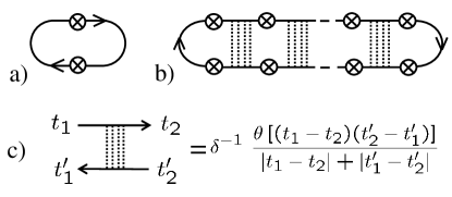
Figure 1: Diagram a) represents the lowest order correction in tunneling conductance $g$ to the partition function, Eq. (9). The solid lines denote the propagator of electrons, the crossed circles stand for the phase dependent tunnelling matrix elements $t_{ij}e^{i\phi_{ij}(\tau)}.$ Diagram b) describes a higher order correction in tunnelling matrix elements $t_{ij}$ that includes impurity averaging within each grain. The dotted lines represent impurity scattering. The diagram c) shows the zero dimensional diffuson in time representation.

The system of weakly coupled metallic grains is described by the Hamiltonian

$$\hat{H}=\hat{H}_{0}+\hat{H}_{c}+\sum_{ij}\,t_{ij}\,\hat{\psi}^{\dagger}(r_{i})\,\hat{\psi}(r_{j}),$$ (5a)

where $$t_{ij} r_{i} r_{j} i j \hat{H}_{0} \hat{H}_{c} \mu_{i}$$ is the tunneling matrix element corresponding to the points of contact and of th and th grains. The Hamiltonian in the r. h. s. of Eq. (5a) describes noninteracting isolated disordered grains. The term includes the electron Coulomb interaction and the local external electrostatic potential on each grain

$$\hat{H}_{c}=\frac{e^{2}}{2}\sum_{ij}\,\hat{n}_{i}\,C_{ij}^{-1}\,\hat{n}_{j}+\sum_{i}\mu_{i}\hat{n}_{i},$$ (5b)

where $C_{ij}$ is the capacitance matrix and $\hat{n}_{i}$ is the operator of electron number in the $i$th grain. The Coulomb interaction term written in a Lagrangean form can be decoupled with the help of the potential field $V_{i}(\tau)$:

$${\cal L}_{c}=-{1\over{2e^{2}}}\,\sum_{ij}[V_{i}+i\mu_{i}]\,C_{ij}\,[V_{j}+i\mu_{j}]-i\sum_{i}n_{i}V_{i},$$ (6)

where $n_{i}=n_{i}(\tau)$ is the electron density field. The last term in the r. h. s. of Eq. (6) can be absorbed by the fermion gauge transformation $\psi_{i}(\tau)\to\psi_{i}(\tau)\,e^{-i\,\phi_{i}(\tau)},$

$$\;\;\;\;\;\phi_{i}(\tau)=\int_{-\infty}^{\tau}V_{i}(\tau^{\prime})d\tau^{\prime},$$ (7)

such that charge action becomes

$${\cal L}_{c}=-{1\over{2e^{2}}}\,\sum_{ij}[V_{i}+i\mu_{i}]\,C_{ij}\,[V_{j}+i\mu_{j}].$$ (8)

Since the action of an isolated grain is gauge invariant the phases $\phi_{i}(\tau)$ enter the full Lagrangean of the system only through the tunnelling matrix elements $t_{ij}\to t_{ij}\,e^{i\phi_{ij}(\tau)},$ where $\phi_{ij}(\tau)=\phi_{i}(\tau)-\phi_{j}(\tau)$ is the phase difference of the $i$th and $j$th grains. We will construct the effective charging functional using the diagrammatic expansion of the partition function $Z$ in tunnelling matrix elements Beloborodov01 . The lowest order correction $Z_{1}$ to the partition function $Z$ defined as $Z=Z_{0}(1+Z_{1}+...)$ with $Z_{0}$ being the partition function of the isolated grains is given by the diagram shown in Fig. 1a. The correction $Z_{1}$ at zero temperature is given by the expression

$$Z_{1}[\phi]={1\over{2\pi}}\sum\limits_{\langle ij\rangle}g_{ij}\int\limits_{-\infty}^{+\infty}\,d\tau_{1}\,d\tau_{2}{{e^{i\phi_{ij}(\tau_{1})-i\phi_{ij}(\tau_{2})}}\over{(\tau_{1}-\tau_{2})^{2}}},$$ (9)

yet to be averaged over the phases $\phi_{i}(\tau).$ The disconnected diagrams must also be included in the partition function such that the complete partition function that takes into account nearest neighbor electron tunneling becomes

$$Z_{NN}=Z_{0}\,\sum_{k=1}^{\infty}\,\langle\;Z_{1}^{k}[\phi]\;\rangle\,/\,k!\,.$$ (10)

Here the angular brackets stand for the averaging over the phase fields $\phi_{i}(\tau)$ with the charging action (8).

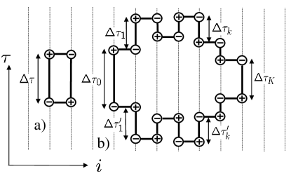
Figure 2: Illustration of the mapping of a quantum granular array model onto the classical model of the charges imbedded into the electron world lines forming loops. Figure (a) describes a quadruple while figure (b) represents the K-th order loop. Though the illustration is shown for the case of $1+1$ dimensions ($1d$ granular array) generalization to higher $d+1$ dimensions is straightforward.

Equation (10) coincides with the partition function obtained from the phase functional of Refs. AES, ; Efetov02, by expansion in small tunneling conductance $g.$ Integration over the phase fields $\phi_{i}(\tau)$ can be implemented exactly for each term in the expansion (10) using Eqs. (6) and (7) with the help of the formula

$$\left\langle e^{i\sum_{n}\phi_{i}(\tau_{n})e_{n}}\right\rangle=e^{-U},$$ (11)

where $U$ can be viewed as a Coulomb energy of a system of classical charges in a space with one extra time dimension interacting via the 1d Coulomb potential  temperature

$$U={1\over 2}\sum_{n_{1},n_{2}}E_{c}^{i_{n_{1}}i_{n_{2}}}|\tau_{n_{1}}-\tau_{n_{2}}|\,e_{n_{1}}\,e_{n_{2}}+\sum_{n}\mu_{i_{n}}\tau_{n}e_{n}.$$ (12)

The physical interpretation of Eq. (12) is as follows: the charges $e_{n}=\pm 1$ interact via the 1d Coulomb potential along the time direction while the strength of the interaction is given by the charging energy $E_{\scriptscriptstyle C}^{ij}=e^{2}C^{-1}_{ij}/2$. In addition, there is a linear growing potential $\mu_{i}\tau$ that can be viewed as a local constant electric field $\mu_{i}$ applied in a time direction.

The partition function, Eq. (10), of the quantum problem under consideration in the nearest neighbor electron tunneling approximation can be presented as a partition function of classical charges that appear in quadruples as shown in Fig. 2a. Each quadruple has its “internal” energy ${\cal E}^{(1)}_{n}$, where the upper index stands for quadruple approximation, that comes from the electron Green function lines in Fig. 1a

$${\cal E}^{(1)}_{n}=\ln[2\pi(\Delta\tau_{n})^{2}/g_{n}].$$ (13)

Here $\Delta\tau_{n}$ is the size of the $n$th quadruple in the $\tau-$ direction in Fig. 2a, $g_{n}$ is the tunneling conductance between the sites occupied by the quadruple and all charges are subject to the Coulomb interaction and local potentials in accordance with Eq. (12). Thus the total energy of a system of N quadruples can be written as

$$E^{(1)}=\sum_{n=1}^{N}{\cal E}^{(1)}_{n}+U_{4N},$$ (14)

where ${\cal E}^{(1)}_{n}$ is the internal energy of the $n$th quadruple and $U_{4N}$ is the static Coulomb energy of 4N charges that form N quadruples defined by Eq. (12). We notice that the different quadruples interact with each other only through the Coulomb part of the energy $U.$ The model (14) can be understood as a classical analog of the phase functional of Ref. AES, and thus it has the same region of applicability. We see that within this approximation the hopping conductivity obviously cannot be described and that higher order tunnelling events must be included.

The advantage of mapping the original quantum model on the classical electrostatic system is that it allows to include the higher order sequential tunneling processes shown in Fig. 2b in essentially the same way as the nearest neighbor hopping. The higher order diagrams include the single grain diffusion propagator $D_{0}=2\pi\delta^{-1}/|\omega_{1}-\omega_{2}|$ that having being transformed into the time representation result in the expression shown in Fig. 1c. Each tunneling matrix element contains phase variables as $t_{ij}e^{i\phi_{ij}(\tau)}.$ Thus, the diagram in Fig. 1b can be presented as a charge loop shown in Fig. 2b. The charges interact electrostatically and are subject to the local potentials according to Eq. (12). The internal energy of a single $K-$th order loop is

$${\cal E}^{(K)} = \ln[2\pi K/g_{0}]-\sum_{k=1}^{K-1}\ln[g_{k}\delta/2\pi]+\ln|\Delta\tau_{0}|$$ (15)

$$+\ln|\Delta\tau_{K}|+\sum_{k=1}^{K-1}\ln(|\Delta\tau_{k}|+|\Delta\tau_{k}^{\prime}|),$$

where the time intervals $\Delta\tau$ and $\Delta\tau^{\prime}$ shown in Fig. 2b have opposite signs.

Now we show how the effective classical model can be used to derive the tunnelling probability through several grains that is the key quantity for understanding the hopping conductivity regime. Let us consider two sites where the local Coulomb gap is absent. In our model it means that the Coulomb energy on these two sites is compensated by the external local potential $\mu_{i}.$ Thus, removing the charge from the grain $i_{0}$ as well as placing the charge on the grain $i_{\scriptscriptstyle K}$ does not cost any Coulomb energy. The electron loops that appear in the classical representation can be viewed as electron worldliness. Thus the probability of tunneling between two sites is given by the free energy of the configuration shown in Fig. 2b. The lower part in Fig. 2b represents the tunneling amplitude $A$ from the site $i_{0}$ to the site $i_{\scriptscriptstyle K}$ while the upper part represents the inverse process. The probability $P=A^{*}A$ is given by the whole loop while the internal energy corresponding to the initial and final states should not be counted.

The contribution of the loop of the K-th order shown in Fig. 2b can be calculated easily for the case of a diagonal Coulomb potential $E_{\scriptscriptstyle C}^{ij}=\delta_{ij}E_{\scriptscriptstyle C}^{i}.$ In this case integrations over the time intervals $\Delta\tau_{k}$ and $\Delta\tau_{k}^{\prime}$ can be done independently and the tunneling probability $P$ is given by the product of sequential probabilities

$$P_{k}={{g_{k}\delta}\over{2\pi}}\int_{\tau_{1},\tau_{2}>0}d\tau_{1}d\tau_{2}{{e^{-E^{+}_{k}\tau_{1}}+e^{-E^{-}_{k}\tau_{2}}}\over{\tau_{1}+\tau_{2}}}$$ (16)

resulting in expression for $P_{k}$ given by Eq. (2).

In the presence of the long range Coulomb interactions the situation is more complicated since the integrals over variables $\Delta\tau_{k},\Delta\tau^{\prime}_{k}$ cannot be taken on each site $k$ independently. However one can estimate the tunnelling probability by finding its upper and lower limits: Indeed, certainly just neglecting the long range part of the potential (as we did above) one gets the upper boundary. The lower boundary can be obtained by considering such trajectories where all $\Delta\tau_{k}$ are of the same sign. In such a case the electric field created by the charges on step $k$ do not interfere with other charges and thus one can implement integrations independently. This will give a lower boundary for the tunnelling probability which is about a factor 2 smaller than the tunnelling probability $P_{k}$ obtained neglecting the long range part of the Coulomb potential. This results in the boundaries of the pre factor $0.5\lesssim c<1.0.$

The above derivation of tunnelling amplitudes was done for the zero temperatures case phonons . Of course the finite temperatures and the presence of phonons are necessary for the realization of the Mott-Efros-Shklovskii mechanism. While there is a temperature interval where temperature effects appear only as a pre-exponential factor and do not interfere to tunnelling probabilities, the extension of the developed method to finite temperatures remains an important task. At zero temperature the system occupies the unique ground state, whereas at finite temperatures the exited states must be included as well. Such exited states can be described by the introduction of winding numbers representing (after Poisson re-summation) the static charges in the system. This generalization however goes beyond the scope of the present Letter and will be a subject of forthcoming publication.

In conclusion, we have developed the technique enabling quantitative description of hopping conductivity of granular conductors in a low, $g\ll 1$, tunneling conductance regime and derived the Coulomb blockade-governed VRH conductivity $\sigma\propto\exp[-(T_{\circ}/T)^{1/2}]$ of granular materials. The essential feature of our approach is representation of sequential intergranular quantum tunneling of the electrons as trajectories of charged classical particles in a $d+1$ dimensional system.

We thank Y.M. Galperin and Sergey Pankov for useful discussions. This work was supported by the U.S. Department of Energy, Office of Science via the contract No. W-31-109-ENG-38.

References

- (1) K. B. Efetov and A. Tschersich, Europhys. Lett. 59, 114, (2002); Phys. Rev. B 67, 174205 (2003).
- (2) I. S. Beloborodov, K. B. Efetov, A. V. Lopatin and V. M. Vinokur, Phys. Rev. Lett 91, 246801 (2003).
- (3) M. V. Feigel’man, A. S. Ioselevich, and M. A. Skvortsov, Phys. Rev. Lett 93, 136403 (2004).
- (4) I. S. Beloborodov, A. V. Lopatin, and V. M. Vinokur, Phys. Rev. B 70, 205120 (2004).
- (5) J. Zhang and B. I. Shklovskii, Phys. Rev. B 70, 115317 (2004).
- (6) A. Gerber et al, Phys. Rev. Lett. 78 , 4277 (1997).
- (7) R. W. Simon et al, Phys. Rev. B 36, 1962 (1987).
- (8) P. Sheng, B. Abeles, and Y. Arie, Phys. Rev. Lett. 31, 44 (1973); B. Abeles, P. Sheng, M. D. Coutts, and Y. Arie, Adv. Phys. 24, 407 (1975).
- (9) B. I. Shklovskii and A. L. Efros, Electronic properties of Doped Semiconductors, Springer-Verlag, New York, 1988).
- (10) L. Efros and B. I. Shklovskii, J. Phys. C 8, L49 (1975).
- (11) N. F. Mott, Adv. Phys. 16, 49 (1967).
- (12) D. A. Averin and Yu. V. Nazarov, Phys. Rev. Lett. 65, 2446 (1990).
- (13) V. Ambegaokar, U. Eckern, and G. Schön, Phys. Rev. Lett. 48, 1745 (1982); for review see G. Schön and A. D. Zaikin, Phys. Rep. 198, 237 (1990).
- (14) A. Schmid, Phys. Rev. Lett. 51, 1506 (1983).
- (15) This estimate for reduces to that adapted in Ref. Shklovskii04, if one takes and the number of channels .
- (16) I. S. Beloborodov, K. B. Efetov, A. Altland and F. W. J. Hekking, Phys. Rev. B 63, 115109 (2001).
- (17) We use the dimensionless units for energy of the classical model assuming that the effective temperature
- (18) This is justified since the characteristic time scale involved in Eq. (16) for tunneling probability is of the order of inverse charging energy that is much shorter than the inverse temperature.