Phase transition in a directed traffic flow network

Abstract

The generic feature of traffic in a network of flowing electronic data packets is a phase transition from a stationary free-flow phase to a continuously growing congested non-stationary phase. In the most simple network of directed oriented square lattice we have been able to observe all crucial features of such flow systems having non-trivial critical behavior near the critical point of transition. The network here is in the shape of a square lattice and data packets are randomly posted with a rate $\rho$ at one side of the lattice. Each packet executes a directed diffusive motion towards the opposite boundary where it is delivered. Packets accumulated at a particular node form a queue and a maximum of $m$ such packets randomly jump out of this node at every time step to its neighbors on a first-in-first-out (FIFO) basis. The phase transition occurs at $\rho_{c}=m$. The distribution of travel times through the system is found to have a log-normal behavior and the power-spectrum of the load time-series shows $1/f$ like noise similar to the scenario of Internet traffic.

I Introduction

The transport of matter and propagation of information in biological, social and electronic communication systems etc. remains significantly important in different branches of physics, more generally in natural science since years. Evidently the prime objective is to make the transport or communication processes more efficient in these systems. In particular, one aims at maximizing the flow at the same time minimizing the delivery time and loss and of course robustness against attack and failure. The effect of the local and global topological properties of the system and the microscopic dynamic process involved with the flow are considered as the two basic ingredients of these complex dynamical process.

Research on highway traffic as a field of applied physics is already decades old. Study on information network traffic is comparatively new. It is evident from the empirical observation on Internet traffic Csabai ; Takayasu ; Leland and vehicular flow Kerner in network of highways that both posses similarity in many respects. In highway network it was observed that on increasing the vehicle density a well-defined transition occurs at a critical density separating the free-flow phase and the jammed phase. At the critical point the jam or congestion occurs as back-propagating waves with fractal properties Gabor . In the Internet network it is found that the ping-time statistics, in which the time taken by a packet to move from source to destination and back were measured, show critical dynamics and $1/f$ noise spectrum similar to the scenario of vehicular traffic Csabai .

Observation of real computer network dynamics also reveals following behavior, namely:
i. Distribution of file sizes is log-normal.
ii. Inter-arrival times has a power law distribution.
iii. Traffic load time series data shows $1/f$ type fluctuation near the critical point
iv. ‘Ping’ experiment data shows round-trip time $\tau_{L}$ distribution has a log-normal behavior.

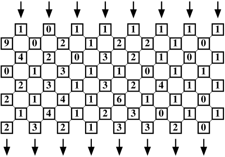
Figure 1: A configuration of the number of data packets at each node of a $8\times 8$ system with the posting rate $\rho=0.8$ in the stationary state.

However the topological structure of the Internet and the highway network are far from being similar. It has been observed that the nodal degree distributions (degree $k$ of a node is the number of links meeting to it) of the Internet Faloutsos and the World-wide web web as well as many other real-world networks have power law tails: $P(k)\sim k^{-\gamma}$ and cannot be modeled by simple random graphs. This is in contrast to the well known random graphs introduced by Erdös and Rényi, whose degree distribution is Poissonian Erdos . Due to the absence of a characteristic value for the nodal degree these new class of networks are called ‘scale-free networks’ (SFN) barabasi ; linked ; review . Barabási and Albert (BA) had grown scale-free graphs where a fixed number of vertices are added at each time and are linked to the growing graph with a linear attachment probability barabasi . On the other hand topological structure of highway network may show small-world behavior in some cases but its degree distribution could not be a power law for practical reasons.

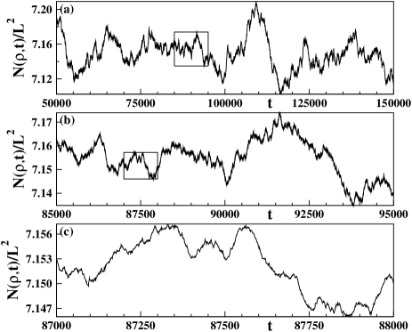
Figure 2: Self-similar fluctuations of the average load per site $N(\rho,t)/L^{2}$ with time $t$ are displayed. (a) Average load of a system of size $L=128$ in the stationary state is plotted for the posting rate $\rho=0.96$ over a range of 100000 time units. (b) Magnification of the boxed region in (a) with the horizontal and vertical scale factors 10 and 2.72 respectively. (c) Magnification of the boxed region in (b) with the horizontal and vertical scale factors 10 and 3.48 respectively.

So the question is whether the self-similarity and long-range dependence of traffic flow and congestion are topological in nature or if they are caused only by the microscopic dynamic properties associated with the generation and flow of traffic, such as posting rate, fluctuations in posting rate or routing schemes.

Traffic system usually involve queues and in the simplest information traffic system consisting of a random information input and a buffer shows a phase transition behavior when the buffer capacity is infinite Takayasu . When the mean input rate is smaller compared to maximum possible output rate, the average accumulation of information at the buffer is finite and this is called the ‘free’ phase. As the mean input rate of information is increased the average accumulation at the buffer increases, and at a critical point the averaged accumulation diverges. The critical point is defined by the simple condition that the mean input rate is equal to the maximum output rate.

This phase transition behavior is local and can occur in any buffer system because of the general nonlinear response of the buffer. But the ‘ping’-experiment indicates phase transition of the whole network due to propagation of congestion among jammed nodes and shows $1/f$ fluctuation at the critical point Takayasu ; Leland . The whole system was also considered as a vast ensemble of ‘phase transition elements’ and the system properties are outcome of the interactions between these individual ‘elements’ Takayasu1 .

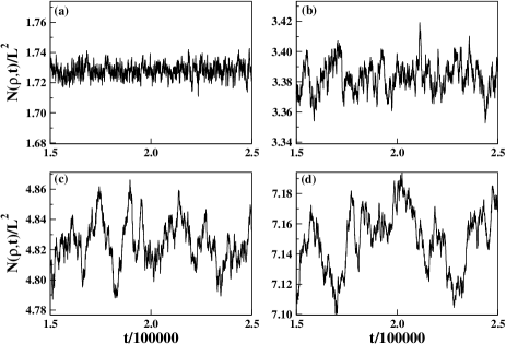
Figure 3: These plots show that as the posting rate $\rho$ approaches the critical posting rate $\rho_{c}$ the fluctuation of the average load per site increases as well as long-range correlation develops. For a system of size $L=128$, average load $N(\rho,t)/L^{2}$ is plotted for 100000 time steps for the posting rates (a) 0.80 (b) 0.90 (c) 0.93 and (d) 0.96 respectively.

In recent studies on different geometries, that is, on linear chain Huisinga and on two-dimensional lattices and on Cayley tree Arenas a sharp transition from free to congested phase is found for routing of packets through shortest paths. In the linear chain the smallest buffer causes jamming Huisinga . In the Cayley tree the role of the node at the top of the hierarchy is crucial for congestion. Also in the case of two-dimensional lattices it is observed that if the packet delivery capacity of the nodes is fixed, or independent of the load on the node then congestion occurs above a specific value of the posting rate $\rho$. Traffic flow has also been studied on scale-free networks Tadic .

In this work we try to address this question of dependence (or independence) of the network traffic flow on topological features and on the details of the dynamic process associated with the generation and flow of traffic. We took a simple network of oriented square lattice and select random diffusion along a preferred direction as the method of routing of data packets (all of same size) and show that this arrangement could generate the main experimental findings of Internet traffic flow.

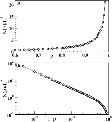
Figure 4: (a) Plot of the average load per site $N(\rho)/L^{2}$ with $\rho$ for $L$ =64 and for $m$ = 1. The growth of average load diverges at the critical point of phase transition at $\rho_{c}=1$. (b) Plot of the average load again but with $1-\rho$ and on a double logarithmic scale, the slope gives the value of the exponent $x\approx 0.96$.

II The model

An oriented square lattice of size $L\times L$ placed on the $x-y$ plane is the network in our model: the lattice sites are the nodes and lattice bonds are the links of the network. The system has a preferential direction, called ‘downward’ direction, imposed along the $-y$ direction such that packets from every site jump with a positive component along the preferred direction. Every node has two neighboring nodes along the preferred direction which are situated at the lower-left (LL) and lower-right (LR) positions. Data packets are posted at a rate $\rho$ only on nodes of the top row of the lattice at $y=L$. Similarly all nodes on the bottom row at $y=0$ are considered as sinks where packets are delivered and therefore disappear from the system. Though the data packets are distinguishable a packet is delivered at any arbitrary sink. In general each of $L^{2}$ nodes is a router which receive, store and forward packets along the preferred direction. There is a limit to the forwarding capacity of each node, a node can forward a maximum of $m$ data packets at a time. Each of these data packets are forwarded to LL or LR nodes randomly with equal probability. Each node receives packets from its two upward neighbors, place them in its buffer maintaining a queue of length $q_{i}(\rho,t)$ and forwards a maximum of $m$ packets at a time from the front of the queue according to the first-in-first-out (FIFO) rule. We further assume that the buffer capacity of each node is infinitely large so that no packet is lost due to filled-up buffer. A single time step during the evolution of the system consists of updating every node of the system for once.

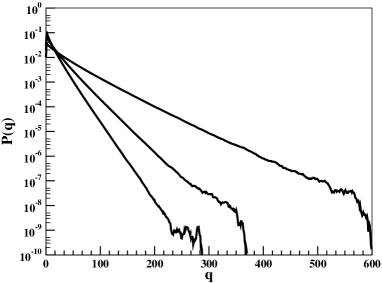
Figure 5: Queue length distribution for a $64\times 64$ lattice with $\rho=$ $0.97,0.98$ and 0.99. Plots indicate exponential decay.

The posting rate $\rho$ of data packets is the only control parameter of the system. Therefore, at each time step, each node of the top row receives a new data packet with a probability $\rho$. The free-flow phase is a stationary state where the average fluxes of the inflow and outflow currents of data packets balance. Once a specific value of $m$ is assigned, magnitudes of these currents can increase at most to $m$. This implies that the critical posting rate $\rho_{c}$ must be equal to $m$. This is supported numerically for a number of values of $m$. In most of our calculations reported below we have used $m=1$.

The total number $N(\rho,t)=\Sigma^{L^{2}}_{i=1}q_{i}(\rho,t)$ of data packets in the network at time $t$ is called the ‘load’ which fluctuates with time but maintains a steady mean value $N(\rho)$ in the stationary free-flow state (Fig. 2 and 3). For a posting rate $\rho>\rho_{c}$ the system switches over to a congested phase and the $N(\rho,t)$ increases indefinitely. Since packets are moving into the system a rate larger than the outflow rate, packets simply pile up in the system and no flow balance is attained. The variation of $N(\rho)$ with $\rho$ is studied. Different packets take different travel times, to reach their destinations. The probability distribution of these travel times is also measured for different $\rho$ values. The nodal queue length distribution of the network is studied for different posting rates.

III Results

The fluctuation of mean load per node or the mean queue length ${\bar{q}(\rho,t)}=N(\rho,t)/L^{2}$ is observed to have a self-similar fluctuation as shown in Fig. 2 for $\rho=0.96$ and $L=128$. In the Fig. 2(a) $N(\rho,t)/L^{2}$ has been plotted with time $t$ over an interval of length $\Delta t=10^{5}$. A small boxed region over a time interval of $\Delta t=10^{4}$ from Fig. 2(a) has been zoomed to Fig. 2(b) using a vertical magnification 2.72 having the same size as of 2(a). Similarly a boxed region over a time interval of $\Delta t=10^{3}$ from Fig. 2(b) has been zoomed to Fig. 2(c) using a vertical magnification 3.48 having the same size as of 2(b). It is evident from the three plots that apart from the stochastic noise present in the system the fluctuation of mean load is self-similar.

In addition the fluctuation of mean load per node becomes stronger and more correlated when $\rho$ approaches the critical posting rate $\rho_{c}$. For small $\rho$ value the load fluctuates around an average value and the fluctuations are also small. It means that the correlation time is short, that is state of the system at a certain time step has very little effect on the states of the system a few time steps away. As $\rho\to\rho_{c}$ the fluctuations in the mean load becomes increasingly stronger and it spreads in a wider region indicating higher correlation in the system. Near $\rho_{c}$ a particular state of the system naturally influences the states of the system far away from it. In Fig. 3 we plot $N(\rho,t)/L^{2}$ for four different posting rates $\rho=0.80,90,0.93$ and 0.96 over an interval of length $10^{5}$ time units and for the system size $L=128$. The width of fluctuation $w(\rho)={\langle{\bar{q}^{2}(\rho,t)}\rangle-\langle{\bar{q}(\rho,t)}\rangle^{2}}$ increases as posting rate increases and also the fluctuation becomes more and more correlated.

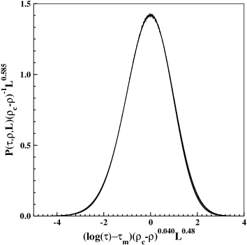
Figure 6: Scaling plot of the data for the distribution of travel times $P(\tau,\rho,L)$ on systems of sizes $L=32$ and 64 for posting rates 0.95, 0.97 and 0.99. The scaled plot fits nicely with a log-normal function.

When $\rho$ is very small the number of packet posted per time step is also very small and the system can deliver it very quickly to the destination. No queue could be formed on the nodes and a packet need not wait in any node while traveling. This is a free-flow phase. But when the posting rate $\rho$ increases, slowly queues are formed and a packet had to wait in queues while traveling and this waiting-time started contributing to the travel time of a packet. But up to certain $\rho$ value the queue length and hence the waiting-time at the nodes fluctuates around an average value, i.e, still the average delivery rate of the system and the average posting rate is equal and there is no growing accumulation of packets in the system. At this stage queues are formed on the nodes and average length of the queues increases with $\rho$ but that average value is not growing with time. But as $\rho\to\rho_{c}$ posting rate becomes equal to the maximum delivery rate (capacity) of the system and beyond that there will be growing accumulation of packets in the system indicating congestion or jammed phase.

Though exactly at $\rho=\rho_{c}=m$ the balance of inflow and outflow fluxes of data packet currents is maintained it is observed that no stationary state is attained at this critical point. This is because not all nodes of the bottom row at $y=1$ receive exactly one data packet each at every time unit, by fluctuation some nodes receive two and some other nodes do not receive any packet at all. Since a node even if received two data packets can deliver at most one packet, some packets must have to stay back in the system ultimately leading to a global congestion. How the mean load per node increases with time at the non-stationary state of $\rho=\rho_{c}$? It is observed that the variation is parabolic i.e., ${\bar{q}}(\rho_{c},t)\sim t^{1/2}$. However for $\rho>\rho_{c}$ the growth is linear in time: ${\bar{q}}(\rho_{c},t)\sim t$.

The time averaged load per node $N(\rho)/L^{2}$ in the free-flow stationary state is calculated for different values of the posting rates $\rho$ and are plotted in Fig. 4(a) for $L=64$. For small values of $\rho$ the load is small and increases slowly. However when $\rho$ approaches $\rho_{c}$ the rate of increase is very fast and diverges. This is seen more explicitly in Fig. 4(b) where $N(\rho)/L^{2}$ is plotted with $\rho_{c}-\rho$ on a double logarithmic scale and a straight line is obtained for $\rho$ close to $\rho_{c}$. The slope of the straight line is 0.98, implying that the load may vary as:

$$N(\rho)/L^{2}\sim(\rho_{c}-\rho)^{-1}$$ (1)

Queue length distribution $P(q)$ of the system which is analogous to jam size distribution in the highway network gives a better understanding of the packet flow scenario. Compared to single-queue theories, here we have many interacting queues in which at each time step a single packet can hop from any queue to any of the two neighboring queues. Thus here apart from the source nodes all other nodes are placed equivalently. They all have only two neighboring nodes as source of data packets. In Fig. 5 we show the plot of $P(q)$ vs. $q$ for $\rho=0.97,0.98$ and 0.99 for $L=64$ on a semi-log scale indicating that the intermediate region of the distribution follow the exponentially decaying distribution $\exp(-q/q_{o}(\rho))$ in general. It has been observed that the dependence $q_{o}(\rho)\sim(\rho_{c}-\rho)^{-1}$ is followed very nicely. The average queue length $\langle q(\rho,y)\rangle$ is also measured as a function of the $y$ co-ordinate and found to vary as $(\rho_{c}-\rho)^{-1}$ independent of $y$ except over a small region near the top level.

The travel time $\tau$ of a data packet is defined as the time spent by the packet in the system which is obviously the difference between the delivery and posting times. Each data packet is given a label and with each node a queue list is associated containing the labels of the data packets in this queue. If the queue length at a node is greater than $m$ then first $m$ packets from the front of the queue are deleted and the queue is shifted $m$ location to the front. Each of these $m$ packets are then randomly routed to one of the LL or LR node. Such a packet is placed at the end of the queue in the new node by the FIFO rule. Intuitively it is easy to understand that for very low posting rates $\rho\to 0$ every data packet makes a hop at every time instant and therefore all $\tau$ values are same and equal to $L$. Consequently the $P(\tau,\rho,L)_{\rho\to 0}=\delta(\tau-L)$. However as $\rho$ increases the queue lengths become larger, as a result travel time increases and its distribution gains a finite width. We have studied in detail the distribution of travel times and its dependence on $\rho$ and $L$ and $P(\tau,\rho,L)$ is observed to follow a combined scaling form over $\rho$ and $L$ as:

$$P(\tau,\rho,L)(\rho_{c}-\rho)^{-1}L^{0.585}\sim{\cal G}[(\log(\tau)-\tau_{m})(\rho_{c}-\rho)^{0.04}L^{0.48}]$$ (2)

The scaling function ${\cal G}(x)$ is seen to follow a log-normal function like:

$${\cal G}(x)=\frac{1}{x\sigma\sqrt{2\pi}}\exp{(-\frac{(\ln x)^{2}}{2\sigma^{2}})}$$ (3)

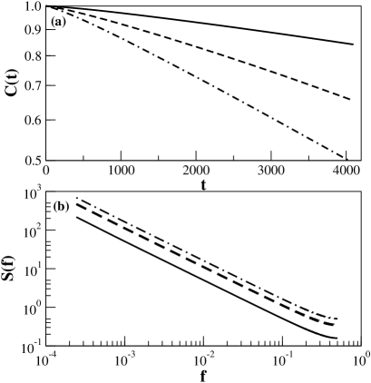
Figure 7: Plot of (a) correlation function $C(t)$ vs. $t$ on a semi-log scale and (b) power spectrum $S(f)$ vs. $f$ on a double log scale for the posting rates: $\rho=$ 0.96 (dot-dashed), 0.97 (dashed) and 0.98 (solid) lines for a system size $L$ = 64.

IV Power-spectral analysis of network time-series

The fluctuation of mean queue length per node $\bar{q}(\rho,t)$ with time depends on the posting rate. In the free-flow stationary state the autocorrelation function of $\bar{q}(\rho,t)$ is defined as:

$$C(\rho,t)=\frac{\langle{\bar{q}(\rho,t^{\prime})\bar{q}(\rho,t+t^{\prime})}\rangle-\langle{\bar{q}(\rho,t^{\prime})}\rangle^{2}}{\langle{\bar{q}^{2}(\rho,t^{\prime})}\rangle-\langle{\bar{q}(\rho,t^{\prime})}\rangle^{2}}$$ (4)

Fourier transform of the autocorrelation function $C(\rho,t)$ is known as the spectral density or power spectrum $S(f)$ defined as

$$S(\rho,f)=\int^{\infty}_{-\infty}e^{-ift}C(\rho,t)dt$$ (5)

For a time series which has no temporal correlation, plot of $S(f)$ against $f$ is independent of $f$. For some other time data series, the power spectrum may vary as a power law: $S(f)\sim f^{-\phi}$. In this case the spectral exponent $\phi$ characterizes the nature of persistence, $\phi=2$ indicates zero correlation associated with Brownian motion, $\phi>2$ indicates positive correlation and persistence and $\phi<2$ represents negative correlation and anti-persistence.

The autocorrelation $C(\rho,t)$ function of the mean queue length in the stationary state is plotted in Fig. 7(a) on a semi-log scale up to $t$=8192 for three values of the posting rate $\rho=0.96,0.97$ and 0.98 calculated on a system size $L=64$. Fourier transformations of these correlation functions are done using ‘xmgrace’ and the power spectrum $S(f)$ is plotted with $f$ on a double logarithmic scale in Fig. 7(b) for all three values of posting rates. The intermediate regimes of the curves are quite straight indicating a power law variation of the power spectrum: $S(f)\sim f^{-\phi(\rho)}$. From Fig. 7(b) we measure the slopes are all nearly same and $\phi(\rho)\approx 1$ indicating $1/f$ noise near critical posting rate $\rho_{c}$ irrespective of the precise value of the posting rate.

Similar autocorrelation functions and associated power spectrum are also calculated for the fluctuation of the length of a single queue $q_{i}(\rho,t)$. The power spectrum is also observed to follow a power law with the spectral exponent value nearly equal to one.

Finally the un-directed version of this problem has also been studied on the square lattice. In this case the data packets are posted at the nodes on the middle row $y=L/2$ and are delivered at the nodes on the top row at $y=L$ and the bottom row $y=1$ with periodic boundary condition applied along the $x$-axis. Each packet executes a simple non-interacting random walk i.e., for each step it selects one of the four neighboring nodes randomly with uniform probability and jumps to that site. As before a similar phase transition is observed from a free-flow state to a congested phase at a specific posting rate $\rho_{c}$. However unlike the previous model, the critical rate $\rho_{c}\to 0$ as $1/L$. This is because a large number of packets simply pile up at the middle line for all values of the posting rates greater than $1/L$. Travel times of packets again follow log-normal distributions and power spectrum also follows a similar power law.

V Conclusion

The properties of traffic of the flow of data packets on a model network of oriented square lattice with random routing scheme largely consistent with the real-world Internet and vehicular traffic flow behaviors. First, it describes the transition from free phase to congested phase with the increase of density of packets separated by a well-defined critical posting rate. Second, it produces the self-similar nature of network workload time series. Third, the long-tailed (log-normal) nature of the travel time distribution is reproduced. Fourth, the power spectral analysis shows $1/f$ type noise confirming long-ranged correlation in the network load time series near criticality.

We thank B.Tadic for useful discussion. GM thankfully acknowledged facilities at S. N. Bose National Centre for Basic Sciences.

Electronic Address: manna@bose.res.in

References

- (1) I. Csabai, J. Phys. A, 27, L417 (1994).
- (2) M. Takayasu, H. Takayasu and T. Sato, Physica. A 233, 824 (1996).
- (3) W. E. Leland, M. S. Taqqu and W. Willinger,IEEE Trans. Networking 2, 1 (1994).
- (4) S. Gábor and I. Csabai, Physica A, 307, 516 (2002).
- (5) B. S. Kerner in Traffic and Granular Flow ’99 ed. by D. Helbing, H. J. Heerman, M. Schreckenberg, D. E. Wolf (Springer, Berlin 2000),pp 253.
- (6) M. Faloutsos, P. Faloutsos and C. Faloutsos, Proc. ACM SIGCOMM, Comput. Commun. Rev., 29, 251 (1999).
- (7) S. Lawrence and C. L. Giles, Science, 280, 98 (1998); Nature, 400, 107 (1999), R. Albert, H. Jeong and A.-L. Barabási, Nature, 401, 130 (1999).
- (8) P. Erdős and A. Rényi, Publ. Math. Debrecen, 6, 290 (1959).
- (9) A.-L. Barabási and R. Albert, Science, 286, 509 (1999); R. Albert and A.-L. Barabási, Rev. Mod. Phys. 74, 47 (2002).
- (10) A.-L. Barabási, Linked: The New Science of Networks, Perseus Publishing, 2002.
- (11) S. N. Dorogovtsev and J. F. F. Mendes, Evolution of Networks, Oxford University Press, 2003; M. E. J. Newman, SIAM Review 45, 167 (2003).
- (12) M. Takayasu, K. Fukuda and H. Takayasu, Physica A, 274, 140 (1999).
- (13) T. Huisinga, R. Barlovic, W. Knospe, A. Schadschneider and M. Schreckenberg, Physica. A. 294, 249 (2001).
- (14) A. Arenas, A. Diaz-Guilera, R. Guimera, Phys. Rev. Lett. 86, 3196 (2001).
- (15) B. Tadic, S. Thurner and G. J. Rodgers, Phys. Rev. E 69, 036102 (2004).