Polymer adsorption onto random planar surfaces:
Interplay of polymer and surface correlations

Abstract

We study the adsorption of homogeneous or heterogeneous polymers onto heterogeneous planar surfaces with exponentially decaying site-site correlations, using a variational reference system approach. As a main result, we derive simple equations for the adsorption-desorption transition line. We show that the adsorption threshold is the same for systems with quenched and annealed disorder. The results are discussed with respect to their implications for the physics of molecular recognition.

I Introduction

Polymer adsorption has been studied intensively in the last decades because of its wide practical applications and rich physics Eisenriegler ; Fleer . The early studies mostly focused on the adsorption onto physically and chemically homogeneous surfaces. In nature, however, real objects are very rarely perfectly homogeneous with ideal geometry. Real substrates usually contain some heterogeneity. Therefore, a number of more recent studies have considered the influence of random heterogeneities on the adsorption transition Balazs/Huang:1991 ; Balazs/Gempe:1991 ; Baumgaertner:1991 ; Sebastian:1993 ; Sumithra:1994 ; Andelman:1993 ; Linden:1994 ; Huber:1998 ; Srebnik:1996 ; Bratko:1997 ; Bratko:1998 ; Chakraborty:1998 ; Srebnik:1998 ; Golumbfskie:1999 ; Srebnik:2000 ; Srebnik:2001 ; Chakraborty_rev ; Moghaddam:2002 ; Lee:2003 ; Moghaddam:2003 ; Genzer:PRE:2001 ; Genzer:ACIS:2001 ; Genzer:JCP:2001 ; Genzer:MTS:2002 .

From a more fundamental point of view, the adsorption of random heteropolymers (RHPs) onto heterogeneous surfaces has attracted much attention, because RHPs serve as biomimetic polymers to study the physics of proteins and nucleic acids. Studying the interaction of RHPs with random heterogeneous surfaces can provide insight into the physics of molecular recognition, a process playing a key role in living organisms (e. g., enzyme-substrate or antigen-antibody interactions).

The present work deals with the adsorption of homopolymers and heteropolymers on surfaces with chemical heterogeneities. As a general rule, the introduction of chemical heterogeneities at constant average load promotes adsorption, since the polymers can adjust their conformations such that they touch predominantly the most attractive surface sites. The adsorption transition is thus shifted to a lower value of the mean polymer/surface affinity. The extent of the shift is determined by the characteristics of the randomness. In the present work, we focus on the influence of correlations on the adsorption transition.

Our study was motivated by the idea that clustering and the interplay of cluster sizes should contribute to molecular recognition. This idea is supported, among other, by a series of recent papers by Chakraborty and coworkers Srebnik:1996 ; Bratko:1997 ; Bratko:1998 ; Chakraborty:1998 ; Srebnik:1998 ; Golumbfskie:1999 ; Srebnik:2000 ; Srebnik:2001 ; Chakraborty_rev . Using different analytical approaches and Monte Carlo (MC) simulations, these authors have established that below the adsorption threshold, statistically blocky polymers favor statistically blocky surfaces over uncorrelated surfaces. They found that, upon increasing the strength of the interactions, the adsorption transition of heteropolymers on heterogeneous surfaces is followed by a second sharp transition, where the polymers freeze into conformations that match the surface pattern. This happens at adsorption energies significantly beyond the adsorption transition. In the biological context, a two-step adsorption process where adsorption is followed by “freezing” possibly describes the physics of protein/DNA recognition, where the protein slides on the DNA for a while before finding it’s specific docking site. For other molecular recognition processes, such as antibody-antigen interactions, it is not only important that a protein adsorbs to a given particle, but equally crucial that it does not adsorb to other objects. In order to assess the importance of cluster size matching in those cases, one must calculate the shift of the adsorption transition as a function of correlation lengths on the polymer and on the surface.

In a previous publication Polotsky:2003 , we have calculated the adsorption/desorption transition of an ideal (non-self-interacting) RHP with sequence correlations on an impenetrable planar homogeneous surface. We have compared two different approaches. First, we have calculated numerically the partition function of a random sample of lattice RHPs Fleer . Provided the sample is sufficiently large, this approach is basically exact. Second, we have applied a reference system approach which was originally developed by Chen Chen:2000 and Denesyuk and Erukhimovich Denesyuk:2000 in a similar context (RHP localization at liquid-liquid interfaces). The second approach allowed to derive an explicit and surprisingly simple expression for the adsorption transition point (repeated here in Eq. (42)), which fitted the numerical results excellently.

Having thus established the validity of the reference system approach, we use it here to study the adsorption of a single Gaussian chain onto a heterogeneous planar surface with exponentially decaying site-site correlations. We consider both homopolymers and random heteropolymers. As in the case of the RHP on an homogeneous surface, we shall derive simple analytic formulae for the adsorption/desorption transition point. This will allow to discuss how surface patchyness influences the adsorption behavior, and whether the interplay of surface and polymer correlations can bring about something relevant to molecular recognition in the vicinity of the adsorption transition.

The problem of adsorption on heterogeneous surfaces has already been considered theoretically by a number of authors, both for homopolymers and heteropolymers (block-copolymers, periodic or random copolymers).

Baumgärtner and Muthukumar Baumgaertner:1991 studied the effect of chemical and physical surface roughness on adsorbed homopolymers. Using MC techniques, they calculated the adsorbed homopolymer amount on chemically heterogeneous surfaces, as a function of temperature and determined the shift of the adsorption-desorption transition temperature with decreasing concentration of adsorbing sites for different chain lengths. In addition, they presented a scaling analysis showing that lateral size of the adsorbed chain $R_{||}$ depends on the distribution of repelling ”impurities” on the adsorbing surface and the strength of their repulsive interaction with the polymer. $R_{||}$ is unaffected by randomness and simply equal to the radius of gyration of a Gaussian chain in two dimensions if impurities are very rare or weak. However, when the impurities are not rare and repulsive barriers are high, $R_{||}$ is of order of the mean distance between neighboring impurities.

Similar conclusions were reached by Sebastian and Sumithra Sebastian:1993 ; Sumithra:1994 , who developed an analytical theory of the adsorption of Gaussian chains on random surfaces, using path integral methods combined with the replica trick and a Gaussian variational approach. They took surface heterogeneity into account by modifying de Gennes’ adsorption boundary condition deGennes:1978 ; deGennes_book , and analyzed the influence of randomness on the conformation of the adsorbed chains.

MC simulations of single polymer adsorption have also been performed by Moghaddam and Wittington Moghaddam:2002 . The sites on the heterogeneous surface were taken to be sticky or neutral for the polymer. The temperature dependencies of the energy and the heat capacity were calculated for different sticker fractions and compared for the cases of quenched and annealed surface disorder. Huber and Vilgis Huber:1998 have studied the case of physically rough surfaces.

The above mentioned works dealt with the single-chain problem. A number of other authors investigated the adsorption from solution onto heterogeneous surfaces using MC simulations Balazs/Huang:1991 ; Balazs/Gempe:1991 , numerical lattice self-consistent field (SCF) calculations Linden:1994 , and an analytical SCF theory Andelman:1993 .

As mentioned earlier, the problem of heteropolymer adsorption on heterogeneous surfaces has been studied extensively by A. Chakraborty and coworkers. Most of the results were summarized in a recent review article Chakraborty_rev, . Srebnik et al. used replica mean field calculations and the replica symmetry breaking scheme to study the adsorption of Gaussian RHP chains for theta solvents Srebnik:1996 and for good solvents Srebnik:2001 . MC simulations combined with simple non-replica calculations allowed to analyze the role of the statistics characterizing the sequence and surface site distribution, and that of intersegment interactions, for the pattern recognition between a disordered RHP and a disordered surface Bratko:1997 ; Bratko:1998 ; Chakraborty:1998 ; Srebnik:1998 ; Golumbfskie:1999 ; Srebnik:2000 .

The adsorption of globular RHPs (e. g., RHPs in a bad solvent) on patterned surfaces has recently been considered by Lee and Vilgis with a variational approach Lee:2003 . A MC simulation study of single RHP chain adsorption onto random surfaces has also been performed by Moghaddam Moghaddam:2003 .

Interesting applications of interactions between copolymers and heterogeneous surfaces have been examined by Genzer Genzer:PRE:2001 ; Genzer:ACIS:2001 ; Genzer:JCP:2001 ; Genzer:MTS:2002 . Using a three dimensional self-consistent field model, he studied the adsorption of A-B copolymers from a mixture of A-B copolymers and A homopolymers onto a heterogeneous planar substrate composed of two chemically distinct regularly or randomly distributed sites. He demonstrated that via substrate recognition, the copolymer can transcribe the two-dimensional surface motif into three dimensions. The specific way the surface motif is translated was shown to be strongly dictated by the copolymer sequence.

The present work differs from all these approaches in that we focus on the adsorption transition, i. e., on the region in parameter space where adsorption just sets in, and that we derive simple analytical expressions for the location of that transition. We shall see that the characteristic features observed in the regime of stronger adsorption do not necessarily carry over to this regime of weak adsorption.

The rest of the paper is organized as follows: Sec. II introduces the model. The free energy calculation based on the reference system approach is explained and carried out in Sec. III. Some aspects of the calculations in this section are very similar to those already described in our earlier publication, Ref. Polotsky:2003, . Therefore, we will skip the corresponding intermediate technical steps and refer the reader to Ref. Polotsky:2003, for more details. Explicit analytic expressions for the adsorption transition point are obtained in Sec. III.5. We summarize and discuss our final expressions in Sec. IV. Some intermediate calculations are described in three Appendices.

II The Model

We consider single Gaussian polymers chain consisting of $N$ monomer units near an impenetrable planar surface. The surface carries randomly distributed sites of different chemical nature. The surface pattern is described by a locally varying interaction parameter $\sigma({\bf x})$. Here ${\bf x}$ denotes Cartesian coordinates $(x,y)$. A particular (hetero)polymer realization is described by a sequence $\xi(n)$, where $n$ indicates the monomer number ($n\in[0:N]$). The strength and the sign of the monomer-surface interaction is determined by the product $\xi(n)\>\sigma({\bf x})$ (a ”+” sign refers to attraction, ”–” to repulsion).

The Hamiltonian of the system can, therefore, be represented as follows:

$$\frac{H}{kT}=\frac{3}{2a^{2}}\int_{0}^{N}dn\left(\frac{\partial{\bf r}}{\partial n}\right)^{2}-\beta\int_{0}^{N}dn\>V(z(n))\>\xi(n)\>\sigma({\bf x}(n))\,,$$ (1)

where ${\bf r}(n)$ is the chain trajectory in the space, ${\bf r}\equiv\{{\bf x},z\}$, $\beta=1/kT$ is the Boltzmann factor, $a$ is the Kuhn segment length of the chain, and $V(z)$ describes the shape of the monomer-surface interaction potential. This potential is taken to be a delta-function pseudopotential shifted at a small but finite distance $z_{0}$ from the impenetrable surface and has the form

$$V(z)=\left\{\begin{array}[]{lc}\delta(z-z_{0})&\mbox{if }z>0\\ +\infty&\mbox{if }z<0\end{array}\right.\,.$$ (2)

The model Hamiltonian (1) can be used to describe interactions of both heteropolymers and homopolymers with both heterogeneous and homogeneous surfaces. Homopolymers are described by a constant sequence function, i.e. $\xi(n)\equiv\xi_{0}$. The sequences $\xi(n)$ of heteropolymers are taken to be randomly distributed according to a Gaussian distribution function

$$P\{\xi(n)\}\propto$$

$$\exp\!\left[-\frac{1}{2}\!\int\!\!\!\!\!\int_{0}^{N}\!\!\!dn_{1}\>dn_{2}(\xi(n_{1})\!-\!\xi_{0})\>c^{-1}(n_{1},n_{2})\>(\xi(n_{2})\!-\!\xi_{0})\right],$$

where $\xi_{0}=\langle\xi\rangle$ characterizes the “mean charge” of the chain, $c(n_{1},n_{2})$ describes sequence correlations, and $c^{-1}$ is the inverse of $c$, defined by $\int\!dn\,c^{-1}(n_{1},n)c(n,n_{2})=\delta(n_{1}-n_{2})$. Here we consider exponentially decaying correlations, i. e.,

$$c(n_{1},n_{2}) \equiv \left\langle(\xi(n_{1})-\xi_{0})(\xi(n_{2})-\xi_{0})\right\rangle$$

$$= c(|n_{2}-n_{1}|)=\Delta_{p}^{2}\>e^{-\Gamma_{p}|n_{2}-n_{1}|}\,.$$

The parameter $\Gamma_{p}$ corresponds to an inverse “contour correlation length“ on the polymer, and $\Delta_{p}$ gives the variance of the single-monomer distribution. The proportionality factor in Eq. (II) is chosen such that $P\{\xi(n)\}$ is normalized. This heteropolymer model also covers homopolymers in the limit $\Delta_{p}\to 0$.

Similarly, the distribution of surface sites on heterogeneous surfaces is chosen to be Gaussian, with the probability

$$P\{\sigma({\bf x})\}\propto$$

$$\exp\!\left[-\frac{1}{2}\!\int\!\!\!\!\!\!\int\!\!d{\bf x}_{1}\>d{\bf x}_{2}\>(\sigma({\bf x}_{1})\!-\!\sigma_{0})\>g^{-1}({\bf x}_{1},{\bf x}_{2})\>(\sigma({\bf x}_{2})\!-\!\sigma_{0})\right]\,,$$

where $\sigma_{0}=\langle\sigma\rangle$ is the mean load of the surface, and the site-site correlation function $g({\bf x}_{1},{\bf x}_{2})$ decays exponentially:

$$g({\bf x}_{1},{\bf x}_{2}) \equiv \left\langle(\sigma({\bf x}_{1})-\sigma_{0})(\sigma({\bf x}_{2})-\sigma_{0})\right\rangle$$

$$= g(|{\bf x}_{1}-{\bf x}_{2}|)=\Delta_{s}^{2}e^{-\Gamma_{s}|{\bf x}_{1}-{\bf x}_{2}|}\,.$$

Here $\Delta_{s}$ is again the variance of the single-site distribution on the surface and $\Gamma_{s}$ is the inverse correlation length of the surface pattern. As before, $g^{-1}({\bf x}_{1},{\bf x}_{2})$ is the inverse function of $g({\bf x}_{1},{\bf x}_{2})$ with the property $\int d{\bf x}\,g^{-1}({\bf x}_{1},{\bf x})g({\bf x},{\bf x}_{2})=\delta({\bf x}_{1}-{\bf x}_{2})$, and $P\{\sigma({\bf x})\}$ is normalized. Homogeneous surfaces are obtained in the limit $\Delta_{s}\to 0$, and are characterized by $\sigma({\bf x})\equiv\sigma_{0}$.

III The Reference System Approach

III.1 Quenched Average via Replica Trick

The free energy of the system is given by the logarithm of the conformational statistical sum averaged over all realizations of the disorder $\beta F=\langle\ln Z\rangle_{\{\sigma({\bf x}),\xi(n)\}}$. Here and below angular brackets $\langle\ldots\rangle$ stand for disorder average. To perform the quenched average we use the well-known replica trick

$$\langle\ln Z\rangle_{\{\sigma({\bf x}),\xi(n)\}}=\lim_{m\to 0}\left\langle\frac{Z^{m}-1}{m}\right\rangle_{\{\sigma({\bf x}),\xi(n)\}}\,.$$ (7)

First we average over the surface disorder $\sigma({\bf x})$. Introducing $m$ replicas of polymer chains and making use of the properties of the Gaussian distribution, Eq. (II), we obtain

$$\langle Z^{m}\rangle_{\sigma({\bf x})} = \int\!\!\prod_{\alpha=1}^{m}\mathcal{D}\{{\bf r}_{\alpha}(n)\}\>\exp\left[-\frac{3}{2a^{2}}\sum_{\alpha=1}^{m}\int_{0}^{N}\!\!dn\left(\frac{\partial{\bf r}_{\alpha}}{\partial n}\right)^{2}\right]$$

$$\times\exp\left[\>\beta\sigma_{0}\int_{0}^{N}\!dn\>\xi(n)\sum_{\alpha=1}^{m}V(z_{\alpha}(n))+\frac{1}{2}\int\!\!\!\!\!\int_{0}^{N}\!\!dn_{1}\>dn_{2}\>\xi(n_{1})\>\xi(n_{2})\>\widehat{g}(n_{1},n_{2})\right]\,,$$

where $\alpha$ is the replica index and $\int\mathcal{D}\{{\bf r}(n)\}$ denotes integration over all possible trajectories ${\bf r}(n)$ of the chain. In Eq. (III.1) we have introduced the notation

$$\widehat{g}(n_{1},n_{2})=$$

$$\beta^{2}\sum_{\alpha,\gamma=1}^{m}V(z_{\alpha}(n_{1}))\>V(z_{\gamma}(n_{2}))\>g({\bf x}_{\alpha}(n_{1})-{\bf x}_{\gamma}(n_{2}))$$

for clarity and future reference.

Next we average over the sequence distribution $\xi(n)$. This affects only the second exponential in (III.1). Again, exploiting the properties of Gaussian integrals, we obtain, after some algebra (see appendix A)

$$\langle Z^{m}\rangle_{\{\sigma({\bf x}),\xi(n)\}} = \int\prod_{\alpha=1}^{m}\mathcal{D}\{{\bf r}_{\alpha}(n)\}\>\exp\left[-\frac{3}{2a^{2}}\sum_{\alpha=1}^{m}\int_{0}^{N}dn\left(\frac{\partial{\bf r}_{\alpha}}{\partial n}\right)^{2}\right]\>\frac{1}{\sqrt{\det K}}$$

$$\times\exp \bigg{[}\sigma_{0}\>\xi_{0}\int\!\!\!\!\!\int_{0}^{N}\!dn_{1}\>dn_{2}\>K^{-1}(n_{1},n_{2})\>\beta\sum_{\alpha=1}^{m}V(z_{\alpha}(n_{2}))\bigg{]}$$

$$\times\exp \bigg{[}\frac{\xi_{0}^{2}}{2}\int\!\!\!\!\!\int\!\!\!\!\!\int_{0}^{N}\!\!dn_{1}\>dn_{2}\>dn_{3}\>K^{-1}(n_{1},n_{2})\>\widehat{g}(n_{2},n_{3})\bigg{]}$$

$$\times\exp \bigg{[}\frac{\sigma_{0}^{2}}{2}\int\!\!\!\!\!\int\!\!\!\!\!\int_{0}^{N}\!\!dn_{1}\>dn_{2}\>dn_{3}\>K^{-1}(n_{1},n_{2})\>c(n_{3}-n_{1})\>\beta^{2}\sum_{\alpha,\gamma=1}^{m}V(z_{\alpha}(n_{2}))\>V(z_{\gamma}(n_{3}))\bigg{]}\,,$$

where $K(n_{1},n_{2})$ is defined as

$$K(n_{1},n_{2})=\delta(n_{1}-n_{2})-\int_{0}^{N}\!\!\!dn_{3}\>\widehat{g}(n_{1},n_{3})\>c(n_{3}-n_{2})\,.$$ (11)

Eq. (III.1) covers the cases of homogeneous and heterogeneous polymers adsorbing on homogeneous and heterogeneous surfaces. If at least one of the partners is homogeneous, the matrix $K$ becomes unity, $K(n_{1},n_{2})=\delta(n_{1}-n_{2})$, and $\det K=1$. If the polymer is homogeneous (a homopolymer), the argument of the last exponential of (III.1) vanishes and we recover Eq. (III.1) in the special case $\xi(n)\equiv\xi_{0}$. If the surface is homogeneous, the argument of the second last exponential in (III.1) vanishes and we recover Eq. (6) of Ref. Polotsky:2003, .

So far the discussion has been fairly general. In the following, we shall mostly restrict ourselves to two specific situations: Homopolymer adsorption on heterogeneous surfaces ($c(n)\equiv 0,K(n_{1},n_{2})=\delta(n_{1}-n_{2})$), and the adsorption of overall neutral heteropolymers on overall neutral heterogeneous surfaces ($\sigma_{0}=\xi_{0}=0$). In the second case, the last three exponentials in Eq. (III.1) can be dropped, and the effect of the disorder comes in solely through the determinant $\det K\neq 1$.

III.2 Definition of the Reference System

To proceed with the calculations, we introduce a reference system Chen:2000 with conformational and thermodynamic properties reasonably close to those of the original system. A natural choice for the reference system is a single homopolymer near an adsorbing homogeneous surface, interacting via an attractive potential of the same form $V(z)$ as in (2), with the interaction strength $w_{0}=\sigma_{0}\>\xi_{0}+v_{0}$. The parameter $v_{0}$ is a variational parameter which can be adjusted such that the reference system is as close as possible to the original one. The Hamiltonian of the reference system has the following form:

$$\frac{H_{0}}{kT}=\frac{3}{2a^{2}}\int_{0}^{N}dn\left(\frac{\partial{\bf r}}{\partial n}\right)^{2}-\beta w_{0}\int_{0}^{N}\,dn\,V(z(n))\,.$$ (12)

The next steps are very similar to those already described in our earlier publication Polotsky:2003 for the case of heteropolymer chain adsorption on a homogeneous planar surface, and shall be only sketched very briefly here. We begin with recasting the quantity $\langle Z^{m}\rangle$ from Eq. (III.1) in the form

$$\langle Z^{m}\rangle=Z_{0}^{m}\big{[}\overline{\exp(A_{m})}\big{]}_{0}^{(m)},$$ (13)

where $Z_{0}$ is the partition function of the reference system, and $[\overline{\cdots}]_{0}^{(m)}$ denotes the chain average with respect to $m$ independent reference chains. The general expression for $A_{m}$ is complicated, but can be obtained from Eq. (III.1) in a straightforward way. In the case of homopolymers adsorbed on a heterogeneous surface, the quantity $A_{m}$ is given by

$$A_{m}=\frac{\xi_{0}^{2}}{2}\int\!\!\!\!\!\int_{0}^{N}dn_{1}\>dn_{2}\>\widehat{g}(n_{1},n_{2})-\beta v_{0}\int_{0}^{N}\!dn\sum_{\alpha=1}^{m}V(z_{\alpha}(n))\,,$$ (14)

and in the case of a neutral heteropolymer on a neutral surface, we get

$$A_{m}=-\frac{1}{2}\ln(\det K)-\beta v_{0}\int_{0}^{N}\!dn\sum_{\alpha=1}^{m}V(z_{\alpha}(n))\,.$$ (15)

The free energy difference between the original system and the reference system is given by:

$$\beta\Delta F = \lim_{m\to 0}(\langle Z^{m}\rangle-Z_{0}^{m})/m$$

$$= \lim_{m\to 0}([\overline{\exp(A_{m})}]_{0}^{(m)}-1)/m\,.$$

Unfortunately, the expression $([\overline{\exp(A_{m})}]_{0}^{(m)}-1)$ cannot be calculated exactly. Therefore, we expand it up to leading order in powers of $v_{0}$, $\widehat{g}$, and $c$ (i. e., $\Delta_{s}$ and $\Delta_{p}$). In the homopolymer case, Eq. (14), this is equivalent to approximating $\exp(A)-1\approx A$. In the heteropolymer case, Eq. (15)) we also have to expand $\ln(\det K)$:

$$\ln(\det K) = \mathop{\rm Tr}\nolimits(\ln K)\approx\mathop{\rm Tr}\nolimits(K-{\bf 1})$$

$$= -\int\!\!\!\!\!\int_{0}^{N}\!dn_{1}\>dn_{2}\>\widehat{g}(n_{1},n_{2})\>c(n_{2}-n_{1})$$

The resulting expression for homopolymers on a heterogeneous surface reads

$$\frac{\beta\Delta F}{N} \approx -\>\beta\>v_{0}[\overline{V(z(n))}]_{0}$$

$$+\>\beta^{2}\>\xi_{0}^{2}\int_{0}^{N}\!\!dk\int\!d{\bf x}^{\prime}\>d{\bf x}^{\prime\prime}\>g({\bf x}^{\prime}-{\bf x}^{\prime\prime})\>[\overline{V(z(n))\delta({\bf x}(n)-{\bf x}^{\prime})V(z(n+k))\delta({\bf x}(n+k)-{\bf x}^{\prime\prime})}]_{0}$$

$$-\>\beta^{2}\>\xi_{0}^{2}\int\!d{\bf x}^{\prime}\>d{\bf x}^{\prime\prime}\>g({\bf x}^{\prime}-{\bf x}^{\prime\prime})\>[\overline{V(z(n))\delta({\bf x}(n)-{\bf x}^{\prime})}]_{0}\;[\overline{V(z(n))\delta({\bf x}(n)-{\bf x}^{\prime\prime})}]_{0}\;N\,.$$

The last term corresponds to contributions from different replicas, whereas the other two belong to single replicas. We have used the fact that averages for different replicas factorize, since different replicated chains are independent in the reference system. Thus $[\overline{\cdots}]_{0}$ denotes the average with respect to a single reference chain, $$[\overline{X}]_{0}=\frac{\int\mathcal{D}\{{\bf r}(n)\}\exp[-\beta H_{0}({\bf r}(n))]X({\bf r}(n))}{\int\mathcal{D}\{{\bf r}(n)\}\exp[-\beta H_{0}({\bf r}(n))]}\,.$$ (19) Likewise, we obtain for neutral heteropolymers on neutral heterogeneous surfaces

$$\frac{\beta\Delta F}{N} \approx -\>\beta\>v_{0}[\overline{V(z(n))}]_{0}$$

$$+\>\beta^{2}\int_{0}^{N}\!\!dk\;c(k)\int\!d{\bf x}^{\prime}\>d{\bf x}^{\prime\prime}\>g({\bf x}^{\prime}-{\bf x}^{\prime\prime})\>[\overline{V(z(n))\delta({\bf x}(n)-{\bf x}^{\prime})V(z(n+k))\delta({\bf x}(n+k)-{\bf x}^{\prime\prime})}]_{0}$$

$$-\>\beta^{2}\int\!d{\bf x}^{\prime}\>d{\bf x}^{\prime\prime}\>g({\bf x}^{\prime}-{\bf x}^{\prime\prime})\>[\overline{V(z(n))\delta({\bf x}(n)-{\bf x}^{\prime})}]_{0}\;[\overline{V(z(n))\delta({\bf x}(n)-{\bf x}^{\prime\prime})}]_{0}\;\int_{0}^{N}\!\!dk\;c(k)$$

As in Eq. (III.2), the first two terms contain contributions from the same replica, and the last term accounts for contributions from different replicas.

At this point, the parameter $v_{0}$ is still a free variational parameter of the theory. In the final step, we will choose it such that the free energies of the reference system and the original system are the same, i.e. $\Delta F=0$.

III.3 Green’s Function and Transition Point of the Reference System

To calculate the averages in (III.2) and (III.2) we need to find the Green’s function of the reference system. It satisfies the following differential equation DoiEdwards ; deGennes_book :

$$-\frac{\partial G}{\partial n}=-\frac{a^{2}}{6}\nabla^{2}G-\beta w_{0}\delta(z-z_{0})G({\bf r},{\bf r}^{\prime};n)\,,$$ (21)

with the appropriate initial and boundary conditions:

$$G({\bf r},{\bf r}^{\prime};0) = \delta({\bf r}-{\bf r}^{\prime})\,,$$ (22)

$$G({\bf r},{\bf r}^{\prime};N)|_{|{\bf r}|\to\infty} = 0\,,$$ (23)

$$G({\bf r},{\bf r}^{\prime};N)|_{z=0} = 0\,.$$ (24)

First, one can separate the variables $x$, $y$ and $z$ writing:

$$G({\bf r},{\bf r}^{\prime};n)=G_{\bf x}({\bf x},{\bf x}^{\prime};n)\>G_{z}(z,z^{\prime};n)\,,$$ (25)

$G_{\bf x}({\bf x},{\bf x}^{\prime};n)$ is the free chain Gaussian distribution in two dimensions:

$$G_{\bf x}({\bf x},{\bf x}^{\prime};n)=\frac{3}{2\pi na}\exp\left[\frac{3({\bf x}-{\bf x}^{\prime})^{2}}{2na^{2}}\right]\,.$$ (26)

For the $z$-dependent part of the Green’s function (25) in the long-chain limit $n\gg 1$, one obtains in the ground-state dominance approximation Aslangul:1995 ; Polotsky:2003

$$G_{z}(z,z^{\prime};n)=\frac{k_{0}/2}{1+(2k_{b}-k_{0})z_{0}}\;e^{-\varepsilon_{0}n}\,.$$

$$\left[e^{-k_{b}|z-z_{0}|}-e^{-k_{b}(z+z_{0})}\right]\;\left[e^{-k_{b}|z^{\prime}-z_{0}|}-e^{-k_{b}(z^{\prime}+z_{0})}\right]$$

where $k_{b}$, determining the ground-state energy ($\varepsilon_{0}=k_{b}a^{2}/6$), is the root of the transcendental equation

$$\frac{2k}{1-e^{-2kz_{0}}}=k_{0}\qquad\mbox{with}\qquad k_{0}=\frac{6\beta w_{0}}{a^{2}}\,.$$ (28)

The complete Green’s function is calculated and discussed in the Appendix B.

The adsorption transition in the reference system takes place when $k_{b}$ and $\varepsilon_{0}$ vanish. This corresponds to the condition Polotsky:2003 $z_{0}k_{0}=1$ or, according to the definition (28) for $k_{0}$, to $6\beta w_{0}/a^{2}=1/z_{0}$.

III.4 Free energy difference between the reference system and the original system

With the results from the previous subsection, we can now evaluate the averages in (III.2) and (III.2). Using the ground-state dominance approximation (III.3) for the Green’s function, we obtain the same result for $[\overline{V(z(n))}]_{0}$ as in Ref. Polotsky:2003, :

$$[\overline{V(z(n))}]_{0}=\frac{2k_{b}^{2}/k_{0}}{1+(2k_{b}-k_{0})z_{0}}\,.$$ (29)

Correspondingly, the averages $[\overline{V(z(n))\delta({\bf x}(n)-{\bf x}^{\prime})}]_{0}$ appearing in the last term of (III.2) and (III.2) are given by

$$\big{[}\overline{V(z(n))\delta({\bf x}(n)-{\bf x}^{\prime})}\big{]}_{0}=\frac{1}{S}\left[\frac{2k_{b}^{2}/k_{0}}{1+(2k_{b}-k_{0})z_{0}}\right]\,.$$ (30)

where $S$ is the surface area. The additional factor $1/S$ in (30), compared to (29), results from the translational freedom of the polymer in the surface plane. Substituting this result into the last term of (III.2) and (III.2) and performing the integration over $\int d{\bf x}^{\prime}\>d{\bf x}^{\prime\prime}$ gives the factor $1/S$. Since $S\to\infty$, this contribution is infinitesimally small and can be omitted in the following calculations.

This seemingly “technical” point has an important physical interpretation. After dropping the last term, Eqs. (III.2) and (III.2) do no longer contain terms with contributions from different replicas. These terms, however, are the only ones which distinguish between quenched and annealed disorder. One can see that by directly carrying out an analogous calculation for annealed disorder. In the annealed case, one has to average directly over the partition function and calculate

$$\beta\delta F_{\mbox{\tiny annealed}}=\ln\langle Z\rangle-\ln Z_{0}=\ln[\overline{\exp(A_{1})}]_{0}.$$ (31)

After expanding up to leading order in powers of $v_{0}$, $\widehat{g}$ and $c$, one obtains the same expressions as (III.2) and (III.2), except that the last term is missing.

The assumption that quenched surface disorder is equivalent to annealed surface disorder has been used in replica mean field calculations Srebnik:1996 and Monte Carlo simulations Bratko:1998 , based on the argument that the chain “samples all significant surface patterns with a probability that asymptotically approaches that of an annealed system in the adiabatic limit” (cited from Ref. Bratko:1998, ). Here we recover this equivalence in the limit of infinite surface area $S$.

We turn to the calculation of $[\overline{\delta({\bf x}(n+k)-{\bf x}^{\prime})V(z(n+k))\delta({\bf x}(n)-{\bf x}^{\prime\prime})V(z(n))}]_{0}$. We assume the validity of the ground-state dominance approximation for the overall chain and for the side subchains. This gives

$$[\overline{\delta({\bf x}(n+k)-{\bf x}^{\prime})V(z(n+k))\delta({\bf x}(n)-{\bf x}^{\prime\prime})V(z(n))}]_{0}$$

$$= \frac{\int d{\bf r}_{1}\,d{\bf r}_{2}\,d{\bf r}_{3}\,d{\bf r}_{4}\,G({\bf r}_{1},{\bf r}_{2};n)\delta({\bf r}_{2}-{{\bf x}^{\prime}\choose z_{0}})G({\bf r}_{2},{\bf r}_{3};k)\delta({\bf r}_{3}-{{\bf x}^{\prime\prime}\choose z_{0}})G({\bf r}_{3},{\bf r}_{4};N-n-k)}{\int d{\bf r}_{1}\,d{\bf r}_{2}\,d{\bf r}_{3}\,d{\bf r}_{4}\,G({\bf r}_{1},{\bf r}_{2};n)G({\bf r}_{2},{\bf r}_{3};k)G({\bf r}_{3},{\bf r}_{4};N-n-k)}$$

$$= \frac{1}{S}G_{\bf x}({\bf x}^{\prime},{\bf x}^{\prime\prime};k)G_{z}(z_{0},z_{0};k)e^{-|\varepsilon_{0}|k}\frac{2k_{b}^{2}/k_{0}}{1+(2k_{b}-k_{0})z_{0}}$$

We consider first the homopolymer case. Inserting (29) – (III.4) into (III.2), we obtain

$$\frac{\beta\Delta F}{N}=\frac{2k_{b}^{2}/k_{0}}{1+(2k_{b}-k_{0})z_{0}}$$

$$\left[\frac{\beta^{2}\xi_{0}^{2}}{S}\int d{\bf x}\,d{\bf x}^{\prime}\;g({\bf x}-{\bf x}^{\prime})\;\mathcal{G}({\bf x},z_{0},{\bf x}^{\prime},z_{0},|\varepsilon_{0}|)|-\beta v_{0}\right].$$

Here

$$\mathcal{G}({\bf r},{\bf r}^{\prime},p) = \int_{0}^{N}dk\,e^{-pk}G({\bf r},{\bf r}^{\prime};k)$$

$$\simeq \int_{0}^{\infty}dk\,e^{-pk}G({\bf r},{\bf r}^{\prime};k)$$

is the Laplace transform of the ”complete” Green’s function $G({\bf r},{\bf r}^{\prime};k)$. We are particularly interested in its value at $z=z^{\prime}=z_{0}$ (i. e., at the level where the potential acts on the chain). The procedure of calculating $\mathcal{G}({\bf x},z_{0},{\bf x}^{\prime},z_{0};|\varepsilon_{0}|)$ is briefly described in the Appendix B. The result can be written in the following integral form

$$\mathcal{G}({\bf x},z_{0},{\bf x}^{\prime},z_{0};|\varepsilon_{0}|)=\frac{6}{a^{2}}\frac{1}{(2\pi)^{2}}\int d{\bf q}\;e^{-i{\bf q}({\bf x}-{\bf x}^{\prime})}$$

$$\times\frac{\sinh\left(z_{0}\sqrt{q^{2}+k_{b}^{2}}\right)}{\sqrt{q^{2}+k_{b}^{2}}e^{z_{0}\sqrt{q^{2}+k_{b}^{2}}}-k_{0}\sinh\left(z_{0}\sqrt{q^{2}+k_{b}^{2}}\right)}$$

where ${\bf q}$ is the two-dimensional vector and $q\equiv|{\bf q}|$. Inserting (III.4) into (III.4) and changing the order of integration over ${\bf q}$ and ${\bf x}$ yields the following expression for the free energy difference between the reference system and a homopolymer adsorbed on a heterogeneous surface:

$$\frac{\beta\Delta F}{N}=\frac{2k_{b}^{2}/k_{0}}{1+(2k_{b}-k_{0})z_{0}}\\ \left[\frac{\beta^{2}\Delta_{s}^{2}\xi_{0}^{2}}{a^{2}}\int_{0}^{\infty}\!\!dq\>\frac{\Gamma_{s}\>q}{\left(q^{2}+\Gamma_{s}^{2}\right)^{3/2}}\frac{6\sinh\left(z_{0}\sqrt{q^{2}+k_{b}^{2}}\right)}{\left(\sqrt{q^{2}+k_{b}^{2}}e^{z_{0}\sqrt{q^{2}+k_{b}^{2}}}-k_{0}\sinh(z_{0}\sqrt{q^{2}+k_{b}^{2}})\right)}-\beta v_{0}\right]$$ (36)

The second case of interest is the neutral heteropolymer on the neutral heterogeneous surface. The difference between the Eqs. (III.2) and (III.2) is due to the monomer-monomer correlation function (II). Inserting expressions (29 - III.4) into (III.2), we obtain

$$\frac{\beta\Delta F}{N}=\frac{2k_{b}^{2}/k_{0}}{1+(2k_{b}-k_{0})z_{0}}\left[\frac{\beta^{2}\Delta_{p}^{2}}{S}\int d{\bf x}\,d{\bf x}^{\prime}\;g({\bf x}-{\bf x}^{\prime})\;\mathcal{G}({\bf x},z_{0},{\bf x}^{\prime},z_{0},\Gamma_{p}+|\varepsilon_{0}|)-\beta v_{0}\right].$$ (37)

This finally leads to

$$\frac{\beta\Delta F}{N}=\frac{2k_{b}^{2}/k_{0}}{1+(2k_{b}-k_{0})z_{0}}\left[\frac{\beta^{2}\Delta_{s}^{2}\Delta_{p}^{2}}{a^{2}}\int_{0}^{\infty}\!\!dq\>\frac{\Gamma_{s}\>q}{\left(q^{2}+\Gamma_{s}^{2}\right)^{3/2}}\frac{6\sinh\left(z_{0}\>\omega(q)\right)}{\left(\omega(q)\>e^{z_{0}\omega(q)}-k_{0}\sinh(z_{0}\>\omega(q))\right)}-\beta v_{0}\right],$$ (38)

with $\omega(q)\equiv\sqrt{q^{2}+6\Gamma_{p}/a^{2}+k_{b}^{2}}$. Note that (36) can formally be obtained from (38) by setting $\Delta_{p}=1$ and $\Gamma_{p}\to 0$. This is, however, not a general rule. The corresponding expression for a heteropolymer adsorbed on a homogeneous surface, Eq. (41) in Ref. Polotsky:2003, is not fully contained in Eq. (38) footnote

III.5 Transition point

Having obtained an approximate expression for the difference $\Delta F$ between the free energies of the original and the reference systems, we adjust the auxiliary parameter $v_{0}$ such that the free energy of the reference system is the best approximation for that of the original one. Thus we require $\Delta F(v_{0}^{*})=0$. For the $\Delta F$ given by (36) or (38), this equation has one trivial solution $k_{b}=0$ or $w_{0}=0$, corresponding to the uninteresting case of a chain which is desorbed in both the original and the reference system. For the other, nontrivial, solution we again consider both cases separately.

In the homopolymer case, the nontrivial solution for $v_{0}$ is given by setting the term in square brackets in Eq. (36) to zero. The transition point for the reference system corresponds to the condition  Polotsky:2003 $z_{0}k_{0}=1$ and $k_{b}\to 0$. Substituting these conditions and introducing, for the sake of convenience, the dimensionless variables

$$\widetilde{v_{0}}=\frac{\beta v_{0}}{a},\quad\widetilde{\sigma_{0}}=\frac{\beta\sigma_{0}}{a},\quad\widetilde{\Delta_{s}}=\frac{\beta\Delta_{s}}{a},\quad$$

$$\widetilde{\Gamma_{s}}=a\Gamma_{s},\mbox{ and}\quad\widetilde{z_{0}}=\frac{z_{0}}{a}$$ (39)

we obtain an equation for the transition point $\widetilde{\sigma_{0}}\xi_{0})^{tr}$ in the random system:

$$(\widetilde{\sigma_{0}}\xi_{0})^{tr}-(\widetilde{\sigma_{0}}\xi_{0})_{\mbox{\tiny homo}}^{tr}=-\beta\widetilde{v_{0}}=-6\>\widetilde{\Delta_{s}}^{2}\xi_{0}^{2}\int_{0}^{\infty}\!\!dq\>\frac{\widetilde{\Gamma_{s}}}{\left(q^{2}+\widetilde{\Gamma_{s}}^{2}\right)^{3/2}}\;\frac{\sinh\left(\widetilde{z_{0}}q\right)}{\left(e^{\widetilde{z_{0}}q}-\sinh(\widetilde{z_{0}}q)/(\widetilde{z_{0}}q)\right)}\;,$$ (40)

where $(\widetilde{\sigma_{0}}\xi_{0})^{tr}_{\mbox{\tiny homo}}\equiv 1/(6\widetilde{z_{0}})$ is the transition point for the homopolymer near an attractive surface. Eq. (40) determines the relation between $\sigma$, $\Gamma_{s}$, and $\Delta_{s}$ that correspond to the adsorption-desorption transition in the original heterogeneous system.

We turn to the case of a neutral heteropolymer on a neutral heterogeneous surface. Here, the nontrivial solution for $v_{0}$, is obtained by setting the term in square brackets in Eq. (38) to zero. We insert again the conditions for the transition point in the reference system, $k_{b}=0$ and $k_{0}\>z_{0}=1$, and switch to the dimensionless variables according to Eq.  (39). The parameters $\Gamma_{p}$ and $\Delta_{p}$ associated with the RHP statistics are already dimensionless. Since $\widetilde{\sigma_{0}}=\xi_{0}=0$, the equation for the transition point then reads:

$$\beta\widetilde{v_{0}}=(\widetilde{\sigma_{0}}\xi_{0})_{\mbox{\tiny homo}}^{tr}=\int_{0}^{\infty}\!\!\!dq\>\frac{6\>\sinh\left(\widetilde{z_{0}}\sqrt{q^{2}+6\Gamma_{p}}\right)}{\left(\sqrt{q^{2}+6\Gamma_{p}}\;e^{\widetilde{z_{0}}\sqrt{q^{2}+6\Gamma_{p}}}-\sinh\left(\widetilde{z_{0}}\sqrt{q^{2}+6\Gamma_{p}}\right)/\widetilde{z_{0}}\right)}\;\frac{\widetilde{\Gamma_{s}}\>q\>\widetilde{\Delta_{s}}^{2}\Delta_{p}^{2}}{\left(q^{2}+\widetilde{\Gamma_{s}}^{2}\right)^{3/2}}.$$ (41)

IV Summary and Discussion

We have used a reference system approach to calculate the adsorption/desorption transition of polymers at surfaces in systems with spatially correlated randomness. The resulting expressions become very elegant in the limit $\widetilde{z_{0}}\ll 1$, i. e., if the range of the surface potential is short compared to the statistical segment length of the polymer. We shall now compile these results, contrast them with the corresponding result in our earlier paper Polotsky:2003, , and discuss them.

We briefly recall the meaning of the different parameters. $\xi_{0}$ denotes the mean polymer charge per segment and $\widetilde{\sigma_{0}}$ the mean surface charge per site; thus the mean affinity between polymer segments and surface sites is given by the parameter $Q=(\widetilde{\sigma_{0}}\xi_{0})$. Randomness shifts the critical affinity parameter at the adsorption transition $Q^{(tr)}$ to lower values, compared to the corresponding value $Q^{(tr)}_{\mbox{\tiny Homo}}$ of a homogeneous system. The shift depends on the variances $\Delta_{p}$ and $\widetilde{\Delta_{s}}$ of the polymer and surface disorder, and on the cluster parameters or inverse correlation lengths $\Gamma_{p}$ and $\widetilde{\Gamma_{s}}$.

The case of random heteropolymers on homogeneous surfaces was already considered in our earlier paper Polotsky:2003 . The transition in the random system is shifted with respect to the homogeneous system by

$$Q^{(tr)}-Q^{(tr)}_{\mbox{\tiny Homo}}=-\Delta_{p}^{2}\widetilde{\sigma_{0}}^{2}\sqrt{\frac{6}{\Gamma_{p}}}.$$ (42)

The case of homopolymers on random surfaces is covered by Eq. (40). In the limit $z_{0}\ll 1$, the integral in (40) can be calculated explicitly and the solution takes the form

$$Q^{(tr)}-Q^{(tr)}_{\mbox{\tiny Homo}}=-\widetilde{\Delta_{s}}^{2}\xi_{0}^{2}\frac{6}{\widetilde{\Gamma_{s}}}.$$ (43)

Heterogeneous polymers on heterogeneous surfaces were discussed in the special case of zero mean affinity. The result, given by Eq. (41), simplifies considerably in the limit $z_{0}\ll 1$. The heteropolymer is adsorbed, if

$$6\frac{\widetilde{\Delta_{s}}^{2}\Delta_{p}^{2}}{\widetilde{\Gamma_{s}}+\sqrt{6\Gamma_{p}}}\geq Q_{\mbox{\tiny Homo}}^{tr}=\mbox{const.}$$ (44)

This defines a phase boundary in the parameter space of variances $\Delta_{p}$ and $\widetilde{\Delta_{s}}$ and cluster parameters $\Gamma_{p}$ and $\widetilde{\Gamma_{s}}$.

In order to complete this compilation of results, we also give the general expression for the shift of the adsorption transition in systems of heterogenous on heterogeneous surfaces (not necessarily neutral). It contains the sum of the three contributions (42), (43), (44), but has one extra term from the expansion of $K^{-1}=\sum_{k=0}^{\infty}(\int_{0}^{N}\!dn_{1}\>\widehat{g}(n_{1},n_{2})\>c(n_{2}-n_{1}))^{k}$ in (III.1). The calculation is absolutely analogous to the one presented in Sec. (III) and yields

$$Q^{(tr)}-Q^{(tr)}_{\mbox{\tiny Homo}} = -\Delta_{p}^{2}\widetilde{\sigma_{0}}^{2}\sqrt{\frac{6}{\Gamma_{p}}}-\widetilde{\Delta_{s}}^{2}\xi_{0}^{2}\frac{6}{\widetilde{\Gamma_{s}}}$$

$$-\widetilde{\Delta_{s}}^{2}\Delta_{p}^{2}\>C+{\cal O}(\widetilde{\Delta_{s}}^{4},\Delta_{p}^{4})$$

where the coefficient $C$ of the higher order term $\widetilde{\Delta_{s}}^{2}\Delta_{p}^{2}$ is given by

$$C = \frac{6}{\widetilde{\Gamma_{s}}+\sqrt{6\Gamma_{p}}}-72\>\widetilde{\sigma_{0}}\xi_{0}\left\{\frac{1}{\sqrt{6\Gamma_{p}}}\Big{(}\frac{1}{\widetilde{\Gamma_{s}}}+\frac{1}{\widetilde{\Gamma_{s}}+\sqrt{6\Gamma_{p}}}\Big{)}\right.$$ (48)

$$\qquad\left.+\frac{1}{\pi\widetilde{\Gamma_{s}}^{2}}G^{22}_{22}\Big{(}\frac{\widetilde{\Gamma_{s}}^{2}}{6\Gamma_{p}}\Big{|}\begin{array}[]{cc}1&1\\ \frac{1}{2}&\frac{3}{2}\end{array}\Big{)}\right\},$$

with the Meijer G function $G$. The calculation of $C$ is shortly sketched in the Appendix C. Note that Eq. (IV)is an implicit equation for $Q^{(tr)}$, because the affinity $Q=(\widetilde{\sigma_{0}}\xi_{0})$ depends both on the mean charge per segment $\xi_{0}$ of the polymer and the mean charge $\widetilde{\sigma_{0}}$ per site on the surface.

The validity of the approximation $\widetilde{z_{0}}\ll 1$ is demonstrated in Fig. 1, which shows some adsorption-desorption transition curves for homopolymers adsorbed on heterogeneous surfaces at different values of $\widetilde{z_{0}}$, as calculated from Eq. (40). As a function of the correlation length $1/\Gamma_{s}$, the curves become straight lines with increasing $1/\Gamma$ with the same slope as the asymptotic curve, Eq. (43). The slope of the curves deviates from the asymptotic value only at small correlation lengths. The simplified expression (43) approximates the full solution (40) reasonably for $\widetilde{z_{0}}<1$. Thus the approximation is justified if the range of the potential is shorter than the statistical segment length. At first sight, this condition seems somewhat arbitrary, given that the value of the statistical segment length $a$ depends on the particular choice of the “segment” unit. One can always increase $a$ by choosing a more coarse grained polymer description, i. e., combining several segments to one new effective segment. The real length scale set by the non-adsorbed polymer is its radius of gyration. Applying the approximation $\widetilde{z_{0}}\ll 1$ in the calculation of the adsorption transition is thus justified whenever the range of the potential is much shorter than the radius of gyration of the polymer.

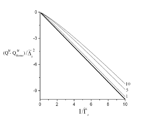
Figure 1: The shift $(Q^{tr}-Q_{\mbox{\tiny Homo}}^{tr})/\widetilde{\Delta_{s}}^{2}$ of the adsorption-desorption transition point for a random surface with exponentially decaying sequence correlations compared to that of a homogeneous attracting surface, vs. correlation length $1/\widetilde{\Gamma_{s}}$, according to Eq. (40). The different curves show the results for different values of $\widetilde{z_{0}}$ as indicated. The bold line corresponds to $\widetilde{z_{0}}=0$, Eq. (43).

Our results can be summarized as follows: The presence of correlations always enhances adsorption. Both increasing the correlation lengths, i. e., decreasing in $\Gamma_{p}$ or $\Gamma_{s}$, and increasing the strength of the correlations (given by $\Delta_{p}$, $\Delta_{s}$) results in a shift of the adsorption transition towards lower affinities.

The results obtained for homopolymers on random surfaces (43) and those for heteropolymers on homogeneous surfaces (42) are very similar. The only difference are the exponents of $\Gamma_{s}$ and $\Gamma_{p}$, which reflect the different ”dimensions” of a planar surface and a linear polymer chain.

The final result (44) for the adsorption of neutral heteropolymers on neutral heterogeneous surfaces gives some particularly interesting information. First, it is worth noting that in Eq. (44), both $\Gamma_{s}$ and $\Gamma_{p}$ enter in the denominator with their ”characteristic” exponents (1 and 1/2, respectively). The other notable feature is that $\Delta_{s}$ and $\Delta_{p}$ enter in (44) as the product of their squares $\widetilde{\Delta_{s}}^{2}\Delta_{p}^{2}$ – a similar dependence on the variances has been observed by Srebnik et al.  Srebnik:1996 for the case of short-range correlated RHPs at a random surface. This means that if the surface (heteropolymer) contains attractive, repelling, and neutral sites and is kept neutral on average, it is preferable to have strongly repelling and strongly adsorbing sites rather than weakly repelling and weakly adsorbing - ”almost neutral” - sites.

We note another interesting property of the considered model. In Sec. III.4, we have already discussed the equivalence of quenched and annealed surface disorder. The argument was based on the fact that all terms related to different replicas in Eqs. (III.2) and (III.2) contain an extra factor $1/S$, which vanishes in the limit of infinite surface area $S$. Technically, the factor $1/S$ reflects the loss of translational freedom of a replica, if it is restricted to stay close to another replica by a coupling through the correlation function $g({\bf x}-{\bf x}^{\prime})$. The argument is thus only valid for surface disorder. In general, quenched and annealed disorder on the polymer are not equivalent.

At the transition point, however, terms related to different replicas always vanish, because every independent replica also contributes a factor $2k_{b}^{2}/k_{0}/(1+(2k_{b}-k_{0})z_{0})\sim 2k_{b}$. In other words, our model calculation predicts that the adsorption threshold is the same for quenched and annealed surface disorder. We believe that this is a general feature of the adsorption transition in disordered systems. Joanny finds the same equivalence when studying the adsorption of polyampholytes on surfaces Joanny:1994 within the Hartree approximation. He claims that it has been conjectured for similar problems by Nieuwenheuizen Nieuwenheuizen . Indeed, polymers and surfaces have only very few contacts at the adsorption transition. It is conceivable that the contacts can be arranged in an optimal way regardless of the particular type of disorder.

If this is true, it has obvious implications for the phenomenon of molecular recognition: It means that studies of the adsorption transition in systems with quenched disorder, averaged with general, unspecific site distribution functions such as Eqs. (II) or (II), can only provide very limited information about specific recognition processes. The adsorption threshold of an annealed polymer, which has had the opportunity to adapt its sequence to the surface, is absolutely equivalent to that of a completely unadapted (quenched) polymer.

We can also use our results to discuss the issue of the interplay between cluster sizes on the surface and the homopolymer. Fig. 2 shows an example of an adsorption phase diagram, obtained from Eq. (44), for neutral heteropolymers on neutral surfaces as a function of the cluster parameters $\Gamma_{p}$ and $\widetilde{\Gamma_{s}}$. The phase boundary does not reflect particular affinities between certain cluster parameters $\Gamma_{p}$ on the polymer and $\widetilde{\Gamma_{s}}$ on the surface. Regardless of the value of $\Gamma_{p}$, the adsorption is always highest at low $\widetilde{\Gamma_{s}}$ and vice versa. We do not observe any complementarity effects.

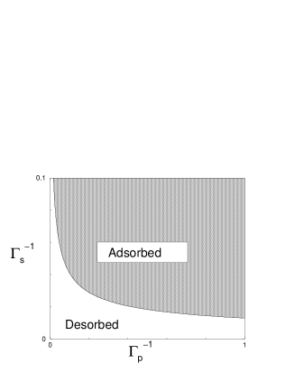
Figure 2: Adsorption transition of neutral heteropolymers on neutral surfaces as a function of $\Gamma_{p}$ and $\widetilde{\Gamma_{s}}$. The parameters are $\widetilde{\Delta_{s}}=\Delta_{p}=1$ and $Q_{\mbox{\tiny Homo}}^{(tr)}=1$.

To summarize, we have been able to derive simple and elegant equations for the adsorption threshold in systems of polymers on surfaces with correlated quenched and annealed disorder. These may be useful for future studies. We have discussed our results in the context of molecular recognition and found that the complex process of pattern recognition between molecules and surfaces close to the adsorption threshold cannot be understood in terms of a simple model with quenched or annealed disorder. We conclude that recognition either takes place at higher affinities, beyond the adsorption threshold, as suggested by Chakraborty et al.  Chakraborty_rev , or has to be studied by more sophisticated models and methods. For example, the situation might change if the probability distribution itself reflects the pattern on the surface. Such considerations shall be the subject of future study.

Acknowlegdement

The financial support of the Deutsche Forschungsgemeinschaft (SFB 613) is gratefully acknowledged. A.P. thanks RFBR (grant 02-03-33127).

Appendix A Performing the Sequence Average

We want to calculate surface disorder average in Eq (III.1). Let us define, for convenience,

$$\bar{\sigma}(n)=\beta\sigma_{0}\sum_{\alpha=1}^{m}V(z_{\alpha}(n))\,,\qquad\bar{\xi}(n)\equiv\xi_{0}$$

and adopt the matrix notation

$$\xi G\xi:=\int\!\!\!\!\!\int_{0}^{N}dn_{1}\>dn_{2}\>\xi(n_{1})\>$$

$$G(n_{1},n_{2})\>\xi(n_{2})\qquad\xi v:=\int_{0}^{N}dn\>\xi(n)v(n)\,.$$

The matrices $c$, $c^{-1}$, and $\widehat{g}$ are symmetric. In order to calculate the sequence average, we need to combine Eqs. (III.1) and (II) and calculate

$$I = \frac{\int\mathcal{D}\{\xi(n)\}\>\exp(\xi\bar{\sigma}+\frac{1}{2}\xi\widehat{g}\xi)\exp(-\frac{1}{2}(\xi-\bar{\xi})c^{-1}(\xi-\bar{\xi}))}{\int\mathcal{D}\{\xi(n)\}\>\exp(-\frac{1}{2}\xi c^{-1}\xi)}$$ (49)

$$= \exp\left[-\frac{1}{2}\bar{\xi}c^{-1}\bar{\xi}+\frac{1}{2}(\bar{\sigma}+\bar{\xi}c^{-1})[c^{-1}-\widehat{g}]^{-1}(\bar{\sigma}+c^{-1}\bar{\xi})\right]$$

$$\times\frac{\int\mathcal{D}\{\xi(n)\}\>e^{-\frac{1}{2}\xi[c^{-1}-\widehat{g}]\xi}}{\int\mathcal{D}\{\xi(n)\}\>e^{-\frac{1}{2}\xi c^{-1}\xi}}$$

The denominator corresponds to the normalization factor in Eq. (II), and the expression $\int\mathcal{D}\{\xi(n)\}$ denotes functional integration in sequence space. To simplify the first exponential on the right hand side of Eq. (49), we define $K={\bf 1}-\widehat{g}c$ (Eq. (11)) and replace $[c^{-1}-\widehat{g}]^{-1}=cK^{-1}$ thus obtain the expression $\exp\left[\bar{\xi}K^{-1}\widehat{g}\bar{\xi}/2+\bar{\sigma}cK^{-1}\bar{\sigma}/2+\bar{\xi}K^{-1}\bar{\sigma}\right]$. This corresponds to the last three exponentials in Eq. (III.1).

To calculate the integrals over sequences $\{\xi(n)\}$ in Eq. (49), we set $n$ back to be a discrete variable, $\int\mathcal{D}\{\xi(n)\}=\int_{0}^{\infty}d\xi_{1}\cdots\int_{0}^{\infty}d\xi_{N}$. This gives

$$\frac{\int\mathcal{D}\{\xi(n)\}\>e^{-\frac{1}{2}\xi[c^{-1}-\widehat{g}]\xi}}{\int\mathcal{D}\{\xi(n)\}\>e^{-\frac{1}{2}\xi c^{-1}\xi}}=\sqrt{\frac{\det(c^{-1})}{\det(c^{-1}-\widehat{g})}}$$

$$= \frac{1}{\sqrt{\det[(c^{-1}-\widehat{g})c]}}=\frac{1}{\sqrt{\det(K)}}\,.$$

The final result, which enters Eq. (III.1), thus reads

$$I=\frac{1}{\sqrt{\det K}}\>\exp\left[\frac{1}{2}\bar{\xi}K^{-1}\widehat{g}\bar{\xi}+\frac{1}{2}\bar{\sigma}cK^{-1}\bar{\sigma}+\bar{\xi}K^{-1}\bar{\sigma}\right].$$ (51)

In matrix notation, it is easy to see that

$$\ln(\det(K)) = \ln(\det(TKT^{-1}))$$

$$= \ln(\prod_{n}\lambda_{n})=\sum_{n}\ln(\lambda_{n})=\mathop{\rm Tr}\nolimits(\ln K)\,,$$

where $T$ diagonalizes $K$, and $\lambda_{n}$ are the eigenvalues of $K$.

Appendix B Complete Green’s Function

Our starting point is the equation (21) with the initial condition (22) and the boundary conditions ((23) and (24)): Laplace transforming with respect to $n$ and taking into account the initial condition (22), we obtain

$$-p\>\mathcal{G}({\bf x},z,{\bf x}^{\prime},z^{\prime};p)+\delta({\bf x}-{\bf x}^{\prime})\delta(z-z^{\prime})$$

$$=-\frac{a^{2}}{6}\nabla^{2}\mathcal{G}-\beta\>w_{0}\>\delta(z-z_{0})\mathcal{G}({\bf x},z,{\bf x}^{\prime},z^{\prime};p)\,,$$

where $\mathcal{G}({\bf x},z,{\bf x}^{\prime},z^{\prime};p)$ is the Laplace transform of $G({\bf x},z,{\bf x}^{\prime},z^{\prime};n)$ with respect to $n$ with the boundary conditions

$$\begin{split}\mathcal{G}({\bf x},z,{\bf x}^{\prime},z^{\prime};p)|_{|{\bf x}|,z\to\infty}&=0,\quad\\ \mathcal{G}({\bf x},z,{\bf x}^{\prime},z^{\prime};p)|_{z\to 0}&=0\end{split}$$ (54)

Firstly, we apply to this equation a Fourier transform with respect to ${\bf x}$ (${\bf x}\to{\bf q}$ and $\mathcal{G}\to\mathscr{G}$)

$$-p\>\mathscr{G}({\bf q},z,{\bf x}^{\prime},z^{\prime};p)+e^{-{\bf q}{\bf x}}\delta(z-z^{\prime})$$

$$= -\frac{a^{2}}{6}\left(-|{\bf q}|^{2}\mathscr{G}+\frac{\partial^{2}\mathscr{G}}{\partial z^{2}}\right)$$

$$-\beta w_{0}\delta(z-z_{0})\mathscr{G}({\bf q},z,{\bf x}^{\prime},z^{\prime};p)$$

and secondly a Laplace transform with respect to $z$ ($z\to s$ and $\mathscr{G}\to g$). $\displaystyle-p\>g({\bf q},s,{\bf x}^{\prime},z^{\prime};p)+e^{-{\bf q}{\bf x}^{\prime}}e^{-z^{\prime}s}=$ $\displaystyle-\>\frac{a^{2}}{6}\left[\left(-|{\bf q}|^{2}+s^{2}\right)g({\bf q},s,{\bf x}^{\prime},z^{\prime};p)\right.$ $\displaystyle\qquad\qquad\left.-s\>\mathscr{G}({\bf q},0,{\bf x}^{\prime},z^{\prime};p)-\mathscr{G}^{\prime}({\bf q},0,{\bf x}^{\prime},z^{\prime};p)\right]$ $\displaystyle-\>\beta\>w_{0}\>e^{-z_{0}s}g({\bf q},z_{0},{\bf x}^{\prime},z^{\prime};p)$ Here $\mathscr{G}^{\prime}$ denotes $\partial\mathscr{G}/\partial z$. This equation can be solved for $g({\bf q},s,{\bf x}^{\prime},z^{\prime};p)$, giving

$$g({\bf q},s,{\bf x}^{\prime},z^{\prime};p)=\frac{\mathscr{G}^{\prime}({\bf q},0,{\bf x}^{\prime},z^{\prime};p)-(6\beta w_{0}/a^{2})\>\mathscr{G}({\bf q},z_{0},{\bf x}^{\prime},z^{\prime};p)\>e^{-z_{0}s}-(6/a^{2})e^{-z^{\prime}s}e^{-{\bf q}{\bf x}^{\prime}}}{s^{2}-|{\bf q}|^{2}-6p/a^{2}}\,.$$ (58)

Taking the inverse Laplace transform of (58) with respect to $s$ and the inverse Fourier transform with respect to ${\bf q}$, we obtain for $\mathcal{G}({\bf x},z_{0},{\bf x}^{\prime},z_{0};p)$:

$$\mathcal{G}({\bf x},z_{0},{\bf x}^{\prime},z_{0};p)=\frac{6}{a^{2}}\frac{1}{(2\pi)^{2}}\int\frac{d{\bf q}\;e^{-i{\bf q}({\bf x}-{\bf x}^{\prime})}\sinh\left(z_{0}\sqrt{q^{2}+6p/a^{2}}\right)}{\sqrt{q^{2}+6p/a^{2}}e^{z_{0}\sqrt{q^{2}+6p/a^{2}}}-k_{0}\sinh\left(z_{0}\sqrt{q^{2}+6p/a^{2}}\right)}$$ (59)

Appendix C Calculation of the higher order term in Eq. IV

Using the matrix notation of the Appendix A, we expand $K^{-1}$ as

$$K^{-1}=\sum_{k=0}^{\infty}(\widehat{g}c)^{k}$$ (60)

and insert it into (III.1). Then, the additional term from this expansion corresponding to the order $\Delta_{p}^{2}\Delta_{s}^{2}$ will have the form:

$$\exp\bigg{[}\sigma_{0}^{2}\xi_{0}^{2}\int_{0}^{N}\!\!dn_{1}\>dn_{2}\>dn_{3}\>\widehat{g}(n_{1},n_{2})\>c(n_{3}-n_{2})\>\beta\sum_{\alpha=1}^{m}V(z_{\alpha}(n_{3}))\bigg{]}$$ (61)

This is equivalent to the following contribution to the $\beta\Delta F/N$ before taking the replica limit $m\to 0$:

$$\beta^{3}\sigma_{0}^{2}\xi_{0}^{2}\int\!d{\bf x}^{\prime}\>d{\bf x}^{\prime\prime}\>g({\bf x}^{\prime}-{\bf x}^{\prime\prime})\>\int_{0}^{N}\!\!dn_{1}\>dn_{2}\>dn_{3}\>c(n_{3}-n_{2})\sum_{\alpha,\gamma,\eta=1}^{m}\overline{V(z_{\alpha}(n_{1}))\delta({\bf x}_{\alpha}(n_{1})-{\bf x}^{\prime})V(z_{\gamma}(n_{2}))\delta({\bf x}_{\gamma}(n_{2})-{\bf x}^{\prime\prime})V(z_{\eta}(n_{3}))}.$$ (62)

Here, $\overline{\cdot}$ denotes the average in a reference system of $m$ independent homogeneous replicated systems. First of all, we notice that only $m$ terms corresponding to replicas with the same indices (i.e. $\alpha=\gamma=\eta$) will contribute to $\Delta F$ in the transition point. After taking the replica limit, we thus have

$$\begin{split}&\beta^{3}\sigma_{0}^{2}\xi_{0}^{2}\int\!d{\bf x}^{\prime}\>d{\bf x}^{\prime\prime}\>g({\bf x}^{\prime}-{\bf x}^{\prime\prime})\>\int_{0}^{N}\!\!dn_{1}\>dn_{2}\>dn_{3}\>c(n_{3}-n_{2})\times\\ &[\overline{V(z(n_{1}))\delta({\bf x}(n_{1})-{\bf x}^{\prime})V(z(n_{2}))\delta({\bf x}(n_{2})-{\bf x}^{\prime\prime})V(z(n_{3}))}]_{0}\end{split}$$ (63)

Note that the monomers $n_{1}$ and $n_{2}$ are ”coupled” in the expression (63) via the site-site correlation function $g$, whereas the correlation between monomers $n_{2}$ and $n_{3}$ is accounted for by the monomer-monomer correlation function $c(n_{3}-n_{2})$. Therefore, one has to take into account the order in the sequence of monomer numbers $n_{1}$, $n_{2}$, and $n_{3}$. There are 3!=6 possible permutations of $n_{1}$, $n_{2}$, and $n_{3}$ but in fact it is sufficient to consider the three possible arrangements schematically shown in Fig. 3.

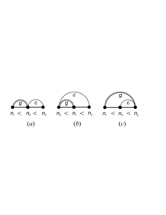
Figure 3: Diagrams contributing to the expression (63). See text for explanation.

The other three are inverse of these ones. We calculate the average in Eq. (63) using the Green’s function of the reference system, like we did in Eq. (III.4), and then integrate it over $\int\!d{\bf x}^{\prime}\>d{\bf x}^{\prime\prime}$ and $\int_{0}^{N}\!\!dn_{1}\>dn_{2}\>dn_{3}$ . These calculations are straightforward and give the following results (in the dimensionless variables $\widetilde{\Gamma_{s}}$ and $\widetilde{\Delta_{s}}$):

$$(a) = \Delta_{p}^{2}\widetilde{\Delta_{s}}^{2}\frac{36}{\sqrt{6\Gamma_{p}}}\>\frac{1}{\widetilde{\Gamma_{s}}}$$ (64)

$$(b) = \Delta_{p}^{2}\widetilde{\Delta_{s}}^{2}\frac{36}{\sqrt{6\Gamma_{p}}}\>\frac{1}{\widetilde{\Gamma_{s}}+\sqrt{6\Gamma_{p}}}$$ (65)

$$(c) = \Delta_{p}^{2}\widetilde{\Delta_{s}}^{2}\frac{36}{\pi\widetilde{\Gamma_{s}}^{2}}\>G^{22}_{22}\Big{(}\frac{\widetilde{\Gamma_{s}}^{2}}{6\Gamma_{p}}\Big{|}\begin{array}[]{cc}1&1\\ 1/2&3/2\end{array}\Big{)}$$ (68)

where $G$ is the Meijer function. Taking into account the double counting (due to inverse sequences) and the prefactor $\widetilde{\sigma_{0}}^{2}\xi_{0}^{2}$ we arrive at the second term in the expression (48) for the coefficient $C$ in Eq. (IV). The first term in $C$ comes, as it has been already noticed, from the expansion (III.2).

References

- (1) E. Eisenriegler, Polymers near surfaces (World Scientific, Singapore, 1993).
- (2) G. J. Fleer, J. M. Scheutjens, M. A. Cohen Stuart, Polymers at interfaces (Chapman & Hall, New York, 1994).
- (3) S. Srebnik, A. Chakraborty, and E.I. Shakhnovich, Phys. Rev. Lett. 77, 3157 (1996).
- (4) D. Bratko, A. Chakraborty, and E.I. Shakhnovich, Chem. Phys. Lett. 280, 46 (1997).
- (5) D. Bratko, A. Chakraborty, and E.I. Shakhnovich, Comp. Theor. Polym. Sci. 8, 113 (1998).
- (6) A. Chakraborty and D. Bratko, J. Chem. Phys. 108, 1676 (1998).
- (7) S. Srebnik, A. Chakraborty, and D. Bratko, J. Chem. Phys. 109, 6415 (1998).
- (8) A. J. Golubfskie, V. S. Pande, and A. K. Chakraborty, Proc. Natl. Acad. Sci. USA 96, 11707 (1999).
- (9) S. Srebnik, J. Chem. Phys. 112, 9655 (2000).
- (10) S. Srebnik, J. Chem. Phys. 113, 9179 (2001).
- (11) A. Chakraborty, Phys. Rep. 342, 1 (2001).
- (12) A. Baumgärtner and M. Muthukumar, J. Chem. Phys. 94, 4062 (1991).
- (13) K.L. Sebastian and K. Sumithra, Phys. Rev. E 47, R32 (1993).
- (14) K. Sumithra and K.L. Sebastian, J. Phys. Chem. 98, 9312 (1994).
- (15) M.S. Moghaddam and S.G. Wittington, J. Phys. A: Math. Gen. 35, 33 (2002).
- (16) G. Huber and T.A. Vilgis, Eur. Phys. J. B 3, 217 (1998).
- (17) A.C. Balazs, K. Huang, and P. McElwain, Macromolecules 24, 714 (1991).
- (18) A.C. Balazs, M.C. Gempe, and Z. Zhou, Macromolecules 24, 4918 (1991).
- (19) C.C. van den Linden, B. van Lent, F.A.M. Leermakers, and G.J. Fleer, Macromolecules 27, 1915 (1994).
- (20) D. Andelman and J.-F. Joanny, J. Phys. II (France) 3, 121 (1993).
- (21) N.-K. Lee and T.A. Vilgis, Phys. Rev. E 67, 050901 (2003).
- (22) M.S. Moghaddam, J. Phys. A: Math. Gen. 36, 939 (2003).
- (23) J.Genzer, Phys. Rev. E 63, 022601 (2001).
- (24) J.Genzer, Adv. Colloid Interface Sci. 94, 105 (2001).
- (25) J.Genzer, J. Chem. Phys. 115, 4873 (2001).
- (26) J.Genzer, Macromol. Theory Simul. 11, 481 (2002).
- (27) A.A. Polotsky, F. Schmid, and A. Degenhard, J. Chem. Phys. 120, accepted (2004).
- (28) Z.Y. Chen, J. Chem. Phys. 112, 8665 (2000).
- (29) N.A. Denesyuk and I.Ya. Erukhimovich, J. Chem. Phys. 113, 3894 (2000).
- (30) P.-G. de Gennes, Rep. Prog. Phys. 32, 187 (1978).
- (31) P.-G. de Gennes, Scaling Concepts in Polymer Physics (Cornell Univ. Press, Ithaca, 1979).
- (32) M. Doi, S.F. Edwards, The Theory of Polymer Dynamics (Oxford Univ. Press, New York, 1986).
- (33) C. Aslangul, Am. J. Phys. 63, 935 (1995).
- (34) This is already obvious from the fact that for heteropolymers, the terms corresponding to different replicas in do not vanish. The contributions to which stem from only one replica can be recovered from Eq. (38) in the limit , , after recognizing that has the properties of a delta-function on the semiaxis .
- (35) J.-F. Joanny, J. Phys. II France 4, 1281 (1994).
- (36) Cited as “private communication” in Ref. Joanny:1994, .