Quasi-particle properties of trapped Fermi gases

Abstract

We develop a consistent formalism in order to explore the effects of density and spin fluctuations on the quasi-particle properties and on the pairing critical temperature of a trapped Fermi gas on the attractive side of a Feshbach resonance. We first analyze the quasi-particle properties of a gas due to interactions far from resonance (effective mass and lifetime, quasi-particle strength and effective interaction) for the two cases of a spherically symmetric harmonic trap and of a spherically symmetric infinite potential well. We then explore the effect of each of these quantities on $T_{c}$ and point out the important role played by the discrete level structure.

1 Introduction

In the last few years the progress in cooling and manipulation of atomic Fermi gases has been impressive [1, 2, 3, 4, 5]. The most notable feature of atomic gases is the presence of scattering resonances (Feshbach resonances), which can be addressed using an external magnetic field. The resonance is induced in the scattering between two atoms in different internal states, typically hyperfine states, and results in the divergence of the two-body $s$-wave scattering length $a_{F}$. Feshbach resonances allow the experimental study of a Fermi gas at various interaction regimes. The crucial feature is that, by varying the value of the scattering length, one can explore different kinds of fermionic superfuidity, ranging from the weak-coupling BCS superfluid, for $a_{F}$ small and negative, to the strong-coupling unitarity regime, $a_{F}\to\infty$, and finally to the Bose-Einstein condensation regime, $a_{F}>0$, where the fermions couple pair-wise to form bosonic molecular bound states. In fact, it has been pointed out some years ago that BCS and BEC are two aspects of one and the same phenomenon, and the basic theory which connects the two was then developed [6, 7, 8]. Recently, this theory came again to the attention of the scientific community in the context of cold atomic Fermi gases [9, 10, 11]. One can show that BCS and BEC appear at the opposite sides of the resonance if one keeps track of the mean-field normal and anomalous pair correlation functions. This essentially corresponds to extending mean-field BCS theory to the whole crossover to BEC. Although the resulting theory is remarkably elegant, it is only qualitatively correct. The absence of important ingredients from the theory as the fluctuating parts of the pair correlation functions and the higher order correlations leads to various flaws in the quantitative predictions. Keeping the full correlations is of course impracticable unless one resorts to quantum Monte Carlo calculations [12, 13, 14]. To pinpoint and understand the important physics contained in the higher order correlations, however, it is also useful to apply approximate methods. This is the line we follow in the present work.

We are interested in improving our understanding of the properties of a Fermi gas as the interaction strength increases originating from the weak-coupling BCS regime. In particular the key quantity we calculate is the critical temperature for pairing $T_{c}$. Moving towards the resonance, higher order correlations and fluctuations over the mean-field become important. One may expect the emission and reabsorption of density and spin fluctuations to play an important role. There are very close analogies between a gas in these conditions and a Fermi liquid. One can build a theory along similar lines introducing the concept of quasi-particles displaying an effective mass, a finite lifetime and an effective interaction due to coupling with fluctuations. The current experiments with Fermi gases have one more particularly interesting aspect in that the atoms are usually confined in harmonic potentials. The finite size plays an important role when the number of particles is not large, as is also the case in optical lattices with few atoms per lattice site, when tunneling between neighboring sites is suppressed and atoms are subjected to an effective harmonic confinement. Both these situations are of interest and have close relations with the physics of finite nuclei and atomic clusters (cf. e. g. [15, 16, 17]). In this article we first develop a formalism appropriate to finite size systems confined by a general, isotropic potential. Subsequently we apply the formalism for the two specific cases of an infinite square well, which we compare with an homogeneous system, and of a spherically symmetric harmonic confinement (cf. also [18]). The results illustrate the central role the discrete level structure plays in determining the properties of these systems. Finally we relate our approach to other calculations for $T_{c}$ (or equivalently for the $T=0$ pairing gap) made in different fields.

The paper in organized as follows. In Sec. 2 we present the theoretical framework. We show the approximations used which lead to the emergence of the renormalized quasi-particle properties, namely the normal self-energy (Sec. 2.1), the anomalous self-energy and the induced interaction (Sec. 2.2), and the one pole approximation (Sec. 2.3). Finally we derive the equations used to calculate $T_{c}$ (Sec. 2.4), including the multipolar expansion appropriate for an isotropic system (Sec. 2.5). In Sec. 3, which is divided into two main subsections, we report the results of the numerical calculations. Sec. 3.1 contains the results for the infinite square well. We discuss the quasi-particle properties and compare the results obtained with those of an infinite system. We also present the calculated values for $T_{c}$. In Sec. 3.2 the same subjects and corresponding results for a harmonically trapped system are presented. Section 4 contains the conclusions. In A.1 details concerning the correlation functions and the linear response of the system for both the uniform and harmonically trapped case are collected.

Before proceeding a remark on notation. In a uniform system the many-body interaction strength is parametrized by $\lambda=gN(0)$, with $g$ being the coupling constant (related to the scattering length $a_{F}$) and $N(0)=mk_{F}/2\pi^{2}\hbar^{2}$ the density of states at the Fermi surface for a single spin orientation. For such system the Fermi momentum $k_{F}$ is related to the uniform density $n$ of the gas by $(3\pi^{2})^{1/3}n^{1/3}$. A similar definition can be introduced for a trapped gas using in place of $n$ the density at the center of the interacting cloud.

2 Theoretical tools

We consider a Fermi gas of $N$ atoms in two internal states with equal numbers ($N/2$) described by the Hamiltonian

$$\hat{H} = \sum_{\sigma=\uparrow,\downarrow}\int d^{3}r\;\hat{\psi}^{\dagger}_{\sigma}({\bf r})(H_{0}-\mu)\hat{\psi}_{\sigma}({\bf r})$$ (1)

$$+ g\int d^{3}r\;\hat{\psi}^{\dagger}_{\uparrow}({\bf r})\hat{\psi}^{\dagger}_{\downarrow}({\bf r})\hat{\psi}_{\downarrow}({\bf r})\hat{\psi}_{\uparrow}({\bf r}).$$

Here $H_{0}=-\hbar^{2}\nabla^{2}/2m_{a}+V_{ext}(r)$, with $m_{a}$ being the atomic mass, and $\uparrow$ and $\downarrow$ conventionally label the two atomic internal states. The only assumptions made at this level on the external potential are that it is isotropic and that it acts in the same way on both atomic states. These assumptions imply that the following relation holds for the chemical potentials $\mu_{\uparrow}=\mu_{\downarrow}=\mu$. Finally, we are here interested in the BCS side of the resonance where $g<0$.

The properties of the system at any given temperature $T$ can be described introducing the normal and anomalous propagators $\mathscr{G}_{\uparrow\uparrow}({\bf r},{\bf r}^{\prime},\omega_{n})$ and $\mathscr{F}_{\uparrow\downarrow}({\bf r},{\bf r}^{\prime},\omega_{n})$. They satisfy the Dyson equations (cf. e.g. ref. [19])

$$\mathscr{G}_{\uparrow\uparrow}({\bf r},{\bf r}^{\prime},\omega_{n}) =\mathscr{G}^{0}_{\uparrow\uparrow}({\bf r},{\bf r}^{\prime},\omega_{n})$$

$$+\displaystyle\int d^{3}s\,d^{3}s^{\prime}\;\mathscr{G}^{0}_{\uparrow\uparrow}({\bf r},{\bf s},\omega_{n})[\Sigma_{\uparrow\uparrow}({\bf s},{\bf s}^{\prime},\omega_{n})\mathscr{G}_{\uparrow\uparrow}({\bf s}^{\prime},{\bf r}^{\prime},\omega_{n})$$

$$-W_{\uparrow\downarrow}({\bf s},{\bf s}^{\prime},\omega_{n})\mathscr{F}^{\dagger}_{\downarrow\uparrow}({\bf s}^{\prime},{\bf r}^{\prime},\omega_{n})]\quad$$

$$\mathscr{F}^{\dagger}_{\downarrow\uparrow}({\bf r},{\bf r}^{\prime},\omega_{n}) =\displaystyle\int d^{3}s\,d^{3}s^{\prime}\;\mathscr{G}^{0}_{\downarrow\downarrow}({\bf s},{\bf r},-\omega_{n})[W_{\downarrow\uparrow}^{\dagger}({\bf s},{\bf s}^{\prime},\omega_{n})\mathscr{G}_{\uparrow\uparrow}({\bf s}^{\prime},{\bf s},\omega_{n})$$

$$+\Sigma_{\downarrow\downarrow}({\bf s}^{\prime},{\bf s},-\omega_{n})\mathscr{F}^{\dagger}_{\downarrow\uparrow}({\bf s},{\bf r}^{\prime},\omega_{n})].$$

The fermionic Matsubara frequency is as usual defined by $\omega_{n}=(2n+1)\pi/\hbar\beta$, where $\beta^{-1}=k_{B}T$, with $T$ being the temperature of the system and $k_{B}$ the Boltzmann constant. $\Sigma_{\sigma\sigma}$ and $W_{\sigma,-\sigma}$ are the normal and anomalous self-energies respectively. Analogous equations to (2) and (2) are satisfied by $\mathscr{G}_{\downarrow\downarrow}$ and $\mathscr{F}_{\uparrow\downarrow}$. The assumption of non-vanishing pair correlations below $T_{c}$ implies a specific choice of gauge in order to break the symmetry of the Hamiltonian. This is implicit in our calculations. We do not need to explicitly worry about the issue because we are only interested in finding the critical temperature $T_{c}$ itself.

In order to further proceed we now need to assume specific approximations for the self-energies.

2.1 The normal self-energy

In this work we account for the possibility for particles to emit and reabsorb density and spin fluctuations and adopt the following set of approximations. We assume $\Sigma_{\uparrow\uparrow}(\omega_{n})=\Sigma^{hf}_{\uparrow\uparrow}+\Sigma^{ph}_{\uparrow\uparrow}(\omega_{n})$, and similarly for $\Sigma_{\uparrow\uparrow}$. The first term corresponds to the ($\omega$-independent) Hartree self-energy [20]:

$$\Sigma_{\uparrow\uparrow}^{hf}({\bf r},{\bf r}^{\prime})=-\frac{g}{\beta}\sum_{n}e^{i\omega_{n}}\mathscr{G}_{\downarrow\downarrow}({\bf r},{\bf r}^{\prime},\omega_{n})\delta({\bf r}-{\bf r}^{\prime})$$ (4)

In practice it is generally not needed to consider the full $\mathscr{G}_{\downarrow\downarrow}$ in Eq. (4). It is instead sufficient to first solve the self-consistent Hartree problem in which $\mathscr{G}_{\downarrow\downarrow}$ is replaced by $\mathscr{G}_{\downarrow\downarrow}^{hf}$ (with $[\mathscr{G}_{\downarrow\downarrow}^{hf}]^{-1}=[\mathscr{G}_{\downarrow\downarrow}^{0}]^{-1}-\Sigma_{\downarrow\downarrow}^{hf}$), and then use this set of functions to calculate the effect of phonons. The self-consistent Hartree problem is solved by expressing the Hartree Green’s functions as

$$\mathscr{G}^{hf}({\bf r},{\bf r}^{\prime},\omega_{n})=\sum_{\nu^{\prime}}\frac{\phi_{\nu^{\prime}}({\bf r})\phi_{\nu^{\prime}}^{*}({\bf r}^{\prime})}{i\hbar\omega_{n}-\xi_{\nu^{\prime}}}.$$ (5)

The quantity $\phi_{\nu}$ is the wave function of the level $\nu$ in the Hartree approximation, and $\xi_{\nu}$ is equal to $\epsilon_{\nu}^{hf}-\mu$, with $\epsilon_{\nu}^{hf}$ being the energy of the level. In Eq. (5) we omitted the spin indices since the Hartree Green’s function is the same for the two species. The Hartree self-energy is on the other hand given by $\Sigma_{\uparrow\uparrow}^{hf}({\bf r},{\bf r}^{\prime})=\delta({\bf r}-{\bf r}^{\prime})\sum_{\nu}|\phi_{\nu}({\bf r})|^{2}n_{F}(\xi_{\nu})$, with $n_{F}(\xi)=1/(e^{\beta\xi}+1)$ being the Fermi distribution function. The chemical potential is obtained imposing

$$N=2\sum_{\nu}\int d^{3}r\;|\phi_{\nu}({\bf r})|^{2}n_{F}(\xi_{\nu}).$$ (6)

(10,20) fermion, label=$\uparrow$, label.side=right, label.dist=20v1,v2 fermionv2,v3 fermion, label=$\uparrow$, label.side=right, label.dist=20v3,v4 wiggly,right=0.8v2,v3 .5w,.05hv1 .5w,.3hv2 .5w,.7hv3 .5w,.95hv4

=      (15,20) fermion, label=$\uparrow$, label.side=left, label.dist=20v1,v2 fermion, label=$\uparrow$, label.side=left, label.dist=20v2,v3 fermion, label=$\uparrow$, label.side=left, label.dist=20v3,v4 fermion,left=0.5,label=$\downarrow$, label.side=right,label.dist=15w1,w2 fermion,left=0.5,label=$\downarrow$, label.side=left,label.dist=15 w2,w1 dashesv2,w1 dashesv3,w2 .1w,.05hv1 .1w,.3hv2 .1w,.7hv3 .1w,.95hv4 .5w,.3hw1 .5w,.7hw2 +       (15,35) fermion, label=$\uparrow$, label.side=left, label.dist=20v1,v2 fermion, label=$\uparrow$, label.side=left, label.dist=20v2,v3 fermion, label=$\uparrow$, label.side=left, label.dist=20v3,v4 fermion, left=0.5,label=$\downarrow$, label.side=right,label.dist=10w1,w2 fermion, left=0.5,label=$\downarrow$, label.side=left,label.dist=10w2,w1 fermion, left=0.5,label=$\uparrow$, label.side=right,label.dist=10w3,w4 fermion, left=0.5,label=$\uparrow$, label.side=left,label.dist=10w4,w3 fermion, left=0.5,label=$\downarrow$, label.side=right,label.dist=10w5,w6 fermion, left=0.5,label=$\downarrow$, label.side=left,label.dist=10w6,w5 dashesv2,w1 dashesw2,w3 dashesv3,w6 dashesw4,w5 .1w,.05hv1 .1w,.2hv2 .1w,.8hv3 .1w,.95hv4 .5w,.2hw1 .5w,.4hw2 .8w,.4hw3 .8w,.6hw4 .5w,.6hw5 .5w,.8hw6 +    …   $(a)$

+      (15,20) fermion, label=$\uparrow$, label.side=left, label.dist=20v1,v2 fermion, label=$\uparrow$, label.side=left, label.dist=20v2,v3 fermion, label=$\uparrow$, label.side=left, label.dist=20v3,v4 fermion, label=$\downarrow$, label.side=right,label.dist=15w2,w1 fermion,right=0.7, label=$\downarrow$, label.side=right,label.dist=15w1,w2 dashesv2,w1 dashesv3,w2 .1w,.05hv1 .1w,.3hv2 .1w,.7hv3 .1w,.95hv4 .5w,.3hw1 .5w,.7hw2 +      (15,25) fermion, label=$\uparrow$, label.side=left, label.dist=20v1,v2 fermion, label=$\uparrow$, label.side=left, label.dist=20v2,v3 fermion, label=$\uparrow$, label.side=left, label.dist=20v3,v4 fermion, label=$\uparrow$, label.side=left, label.dist=20v4,v5 fermion, label=$\downarrow$, label.side=right,label.dist=15w2,w1 fermion, label=$\downarrow$, label.side=right,label.dist=15w3,w2 fermion,right=0.7, label=$\downarrow$, label.side=right,label.dist=15w1,w3 dashesv2,w1 dashesv3,w2 dashesv4,w3 .1w,.05hv1 .1w,.2hv2 .1w,.5hv3 .1w,.8hv4 .1w,.95hv5 .5w,.2hw1 .5w,.5hw2 .5w,.8hw3     +    …     $(b)$

Figure 1: Phonon-induced self-energy $\Sigma^{ph}_{\uparrow\uparrow}({\bf r},{\bf r}^{\prime},\omega_{n})$ (Eqs. (2.1) and (9)). The continuous lines correspond to Hartree Green’s functions $\mathscr{G}^{hf}({\bf r},{\bf r}^{\prime},\omega_{n})$, the dashed lines to the bare interaction $g\delta({\bf r}-{\bf r}^{\prime})$. The self-energy $\Sigma_{\uparrow\uparrow}^{(1)}$ is given by the contributions in $(a)$. $\Sigma_{\uparrow\uparrow}^{(2)}$, which arises from coupling to spin phonons, is given by the diagrams in $(b)$. The diagrams with an even number of bubbles are not included in $(a)$ because the bare interaction acts only between atoms in different internal states.

We deal with the self-energy $\Sigma_{\uparrow\uparrow}^{ph}$ due to coupling with collective modes in the context of the Random Phase Approximation [21]. We thus suppose $\Sigma_{\uparrow\uparrow}^{ph}$ to be given by the sum of the Feynman graphs shown in Fig. 1, where to each fermion line corresponds a $\mathscr{G}^{hf}$ and to each dashed line an interaction $g\delta({\bf r}-{\bf r}^{\prime})$. This part of self-energy can be written as the sum of two contributions $\Sigma_{\uparrow\uparrow}^{(1)}$ and $\Sigma_{\uparrow\uparrow}^{(2)}$ (cf. Fig. 1 $(a)$ and $(b)$ respectively). $\Sigma_{\uparrow\uparrow}^{(1)}$ is given by

$$\Sigma_{\uparrow\uparrow}^{(1)}({\bf r},{\bf r}^{\prime},\omega_{n})-\displaystyle\frac{g^{2}}{\beta}\sum_{\omega_{m}}\mathscr{G}_{\uparrow\uparrow}^{hf}({\bf r},{\bf r}^{\prime},\omega_{n})\Pi_{\downarrow\downarrow}^{r}({\bf r},{\bf r}^{\prime},\omega_{n}+\omega_{m})$$

where $\Pi_{\downarrow\downarrow}^{r}$ is the ring approximation to the correlation function (for all the correlation functions, and their relations, used in this Section we refer the reader to A.1). This can be written as the sum of a density and a spin part:

$$\Pi_{\downarrow\downarrow}^{r}({\bf r},{\bf r}^{\prime},\omega_{m})=\displaystyle{\frac{1}{4}}\Big{\{}\Pi_{\rho}^{r}({\bf r},{\bf r}^{\prime},\omega_{m})+\Pi_{\sigma_{z}}^{r}({\bf r},{\bf r}^{\prime},\omega_{m})\Big{\}},\;$$ (7)

with $\omega_{m}=2m\pi/\hbar\beta$ being a bosonic Matsubara frequency. The second contribution is instead given by:

$$\Sigma_{\uparrow\uparrow}^{(2)}({\bf r},{\bf r}^{\prime},\omega_{n})=-\displaystyle{\frac{g^{2}}{4\beta}}\sum_{\omega_{m}}\mathscr{G}_{\downarrow\downarrow}^{hf}({\bf r},{\bf r}^{\prime},\omega_{n})$$

$$\Big{\{}\Pi_{\sigma_{x}}^{r}({\bf r},{\bf r}^{\prime},\omega_{n}+\omega_{m})+\Pi_{\sigma_{y}}^{r}({\bf r},{\bf r}^{\prime},\omega_{n}+\omega_{m})\Big{\}}.$$ (8)

Combining the two contributions one finds

$$\Sigma^{ph}_{\uparrow\uparrow}({\bf r},{\bf r}^{\prime},\omega_{n})=-\displaystyle{\frac{g^{2}}{4\beta}}\sum_{\omega_{m}}\mathscr{G}^{hf}({\bf r},{\bf r}^{\prime},\omega_{n})$$

$$\times\Big{\{}\Pi_{\rho}^{r}({\bf r},{\bf r}^{\prime},\omega_{n}+\omega_{m})+3\Pi_{\sigma_{z}}^{r}({\bf r},{\bf r}^{\prime},\omega_{n}+\omega_{m})-2\Pi_{\rho}^{0}({\bf r},{\bf r}^{\prime},\omega_{n}+\omega_{m})\Big{\}}$$

$$=-\displaystyle{\frac{g^{2}}{\beta}}\sum_{\omega_{m}}\mathscr{G}^{hf}({\bf r},{\bf r}^{\prime},\omega_{n})\Big{\{}2\Pi_{\uparrow\uparrow}^{r}({\bf r},{\bf r}^{\prime},\omega_{n}+\omega_{m})$$

$$-\Pi_{\uparrow\downarrow}^{r}({\bf r},{\bf r}^{\prime},\omega_{n}+\omega_{m})-\chi_{0}({\bf r},{\bf r}^{\prime},\omega_{n}+\omega_{m})\Big{\}}.$$ (9)

In Eqs. (2.1) and (9) we have used $\Pi_{\sigma_{x}}=\Pi_{\sigma_{y}}=\Pi_{\sigma_{z}}$ and we accounted for the fact that the single bubble diagram belongs both to $\Sigma_{\uparrow\uparrow}^{(1)}$ and to $\Sigma_{\uparrow\uparrow}^{(2)}$ and is therefore doubly counted in a simple summation. For this reason we subtracted the quantity $2\Pi_{\rho}^{0}$ in Eq. (2.1).

It is useful to introduce the spectral representations for the correlation functions:

$$\Pi_{\rho}^{r}({\bf r},{\bf r}^{\prime},\omega_{m})=\int_{0}^{\infty}\frac{d\omega^{\prime}}{\pi}\;{\rm Im}[\Pi_{\rho}^{r}({\bf r},{\bf r}^{\prime},\omega^{\prime})]\frac{2\omega^{\prime}}{\omega_{m}^{2}+\omega^{{}^{\prime}2}},$$ (10)

$$\Pi_{\sigma_{z}}^{r}({\bf r},{\bf r}^{\prime},\omega_{m})=\int_{0}^{\infty}\frac{d\omega^{\prime}}{\pi}\;{\rm Im}[\Pi_{\sigma_{z}}^{r}({\bf r},{\bf r}^{\prime},\omega^{\prime})]\frac{2\omega^{\prime}}{\omega_{m}^{2}+\omega^{{}^{\prime}2}},$$ (11)

$$\Pi_{\rho}^{0}({\bf r},{\bf r}^{\prime},\omega_{m})=\int_{0}^{\infty}\frac{d\omega^{\prime}}{\pi}\;{\rm Im}[\Pi_{\rho}^{0}({\bf r},{\bf r}^{\prime},\omega^{\prime})]\frac{2\omega^{\prime}}{\omega_{m}^{2}+\omega^{{}^{\prime}2}},$$ (12)

where $\Pi_{\rho}^{r}({\bf r},{\bf r}^{\prime},\omega)$, $\Pi_{\sigma_{z}}^{r}({\bf r},{\bf r}^{\prime},\omega)$ and $\Pi_{\rho}^{0}({\bf r},{\bf r}^{\prime},\omega)$ are the retarded correlation functions (obtained using the analytic continuation $\omega_{n}\to\omega+i\eta$), and we have used $\Pi_{i}^{r}({\bf r},{\bf r}^{\prime},\omega)=-\Pi_{i}^{r}({\bf r},{\bf r}^{\prime},-\omega)$.

Inserting these relations, together with Eq. (5), in Eq. (9) and carrying out the frequency summation one finds

$$\Sigma_{\uparrow\uparrow}^{ph}({\bf r},{\bf r}^{\prime},\omega_{n})=-\displaystyle g^{2}\sum_{\nu^{\prime}}\phi_{\nu^{\prime}}({\bf r})\phi_{\nu^{\prime}}^{*}({\bf r}^{\prime})\int_{0}^{\infty}\frac{d\omega^{\prime}}{\pi}\;$$

$${\rm Im}\big{[}2\Pi_{\uparrow\uparrow}^{r}({\bf r},{\bf r}^{\prime},\omega^{\prime})-\Pi_{\uparrow\downarrow}^{r}({\bf r},{\bf r}^{\prime},\omega^{\prime})-\chi_{0}({\bf r},{\bf r}^{\prime},\omega^{\prime})\big{]}$$

$$\times\left(\displaystyle{\frac{n_{B}(\omega^{\prime})+1-n_{F}(\xi_{\nu^{\prime}})}{i\omega_{n}-\hbar^{-1}\xi_{\nu^{\prime}}-\omega^{\prime}}+\frac{n_{B}(\omega^{\prime})+n_{F}(\xi_{\nu^{\prime}})}{i\omega_{n}-\hbar^{-1}\xi_{\nu^{\prime}}+\omega^{\prime}}}\right),\quad$$ (13)

where $n_{B}(\omega)=1/(e^{\beta\hbar\omega}-1)$ is the Bose distribution function.

The self-energy of the quasi-particle in the level $\nu$ is given by $\Sigma^{ph}_{\nu}(\omega_{n})=\int\,d^{3}r\,d^{3}r^{\prime}\,\phi^{*}_{\nu}({\bf r})\phi_{\nu}({\bf r}^{\prime})\Sigma^{ph}({\bf r},{\bf r}^{\prime},\omega_{n})$ and therefore

$$\Sigma^{ph}_{\nu}(\omega_{n})=-\displaystyle{\sum_{\nu^{\prime}}\int_{0}^{\infty}\frac{d\omega^{\prime}}{\pi}\;\sigma_{\nu\nu^{\prime}}(\omega^{\prime})}$$

$$\times{\left(\displaystyle{\frac{1+n_{B}(\omega^{\prime})-n_{F}(\xi_{\nu^{\prime}})}{i\omega_{n}-\hbar^{-1}\xi_{\nu^{\prime}}-\omega^{\prime}}+\frac{n_{B}(\omega^{\prime})+n_{F}(\xi_{\nu^{\prime}})}{i\omega_{n}-\hbar^{-1}\xi_{\nu^{\prime}}+\omega^{\prime}}}\right)},$$ (14)

where

$$\sigma_{\nu\nu^{\prime}}(\omega) =g^{2}\displaystyle\int d^{3}rd^{3}r^{\prime}\;\phi_{\nu^{\prime}}({\bf r})\phi_{\nu}^{*}({\bf r})\phi_{\nu^{\prime}}^{*}({\bf r}^{\prime})\phi_{\nu}({\bf r}^{\prime})$$ (15)

$$\times{\rm Im}\big{[}2\Pi_{\uparrow\uparrow}^{r}({\bf r},{\bf r}^{\prime},\omega)-\Pi_{\uparrow\downarrow}^{r}({\bf r},{\bf r}^{\prime},\omega)-\chi_{0}({\bf r},{\bf r}^{\prime},\omega)\big{]}.\quad$$

2.2 The anomalous self-energy

The anomalous self-energy in Eqs. (2) and (2) is given by (cf. [19])

$$W_{\uparrow\downarrow}({\bf r},{\bf r}^{\prime},\omega_{n})=-\displaystyle\frac{1}{\beta}\sum_{\omega_{m}}V^{eff}_{\uparrow\downarrow}({\bf r},{\bf r}^{\prime},\omega_{m})\mathscr{F}_{\uparrow\downarrow}({\bf r},{\bf r}^{\prime},\omega_{n}+\omega_{m}),$$

where $V^{eff}_{\uparrow\downarrow}$ is an effective interaction between quasi-particles in states $\uparrow$ and $\downarrow$. Accounting also for the possibility for particles to interact exchanging density and spin fluctuations, $V_{\uparrow\downarrow}^{eff}({\bf r},{\bf r}^{\prime},\omega_{m})$ is the sum of two terms: the ($\omega$-independent) bare interaction $g\delta({\bf r}-{\bf r}^{\prime})$ and the induced interaction

$$V^{ind}_{\uparrow\downarrow}({\bf r},{\bf r}^{\prime},\omega_{m})=\displaystyle{\frac{g^{2}}{4}}\big{[}\Pi_{\rho}^{r}({\bf r},{\bf r}^{\prime},\omega_{m})-3\Pi_{\sigma_{z}}^{r}({\bf r},{\bf r}^{\prime},\omega_{m})\big{]}$$ (16)

which corresponds to the diagrams shown in Figure 2.

(10,20) .2w,.1hv1 .8w,.1hv2 .2w,.9hv3 .8w,.9hv4 empty,tension=1.G4 fermion, label=$\uparrow$, label.side=left, label.dist=20v1,G1 fermion, label=$\downarrow$, label.side=right, label.dist=20v2,G2 fermionG4,v3 fermionG3,v4

=       (15,25) fermion, label=$\uparrow$, label.side=left, label.dist=20v1,v2 fermion, label=$\uparrow$, label.side=left, label.dist=20v2,v3 fermion, label=$\downarrow$, label.side=right, label.dist=20v4,v5 fermion, label=$\downarrow$, label.side=right, label.dist=20v5,v6 fermion,left=0.5, label=$\downarrow$, label.side=right, label.dist=10w1,w2 fermion,left=0.5, label=$\downarrow$, label.side=left, label.dist=10w2,w1 fermion,left=0.5, label=$\downarrow$, label.side=left, label.dist=10w3,w4 fermion,left=0.5, label=$\downarrow$, label.side=right, label.dist=10w4,w3 dashesv2,w1 dashesw2,w3 dashesw4,v5 .1w,.05hv1 .1w,.2hv2 .1w,.95hv3 .9w,.05hv4 .9w,.8hv5 .9w,.95hv6 .35w,.2hw1 .35w,.5hw2 .65w,.5hw3 .65w,.8hw4    +   …    (a)

+     (15,20) fermion, label=$\uparrow$, label.side=left, label.dist=20v1,v2 fermion, label=$\uparrow$, label.side=left, label.dist=20v2,v3 fermion, label=$\uparrow$, label.side=left, label.dist=20v3,v4 fermion, label=$\downarrow$, label.side=right, label.dist=20v5,w2 fermionw1,v6 fermion, label=$\downarrow$, label.side=right, label.dist=15w2,w1 dashesv2,w1 dashesw2,v3 .1w,.1hv1 .1w,.3hv2 .1w,.7hv3 .1w,.9hv4 .9w,.1hv5 .9w,.9hv6 .4w,.3hw1 .4w,.7hw2 +        (15,25) fermion, label=$\uparrow$, label.side=left, label.dist=20v1,v2 fermion, label=$\uparrow$, label.side=left, label.dist=20v2,v7 fermion, label=$\uparrow$, label.side=left, label.dist=20v7,v3 fermion, label=$\uparrow$, label.side=left, label.dist=20v3,v4 fermion, label=$\downarrow$, label.side=right, label.dist=20v5,w2 fermionw1,v6 fermion, label=$\downarrow$, label.side=right, label.dist=15w2,w3 fermion, label=$\downarrow$, label.side=right, label.dist=15w3,w1 dashesv2,w1 dashesw2,v3 dashesv7,w3 .1w,.05hv1 .1w,.25hv2 .1w,.75hv3 .1w,.95hv4 .9w,.1hv5 .9w,.9hv6 .1w,.5hv7 .5w,.25hw1 .5w,.75hw2 .5w,.5hw3 +    …    (b)

Figure 2: Phonon-induced interaction $V^{ind}_{\uparrow\downarrow}({\bf r},{\bf r}^{\prime},\omega_{n})$ (see Eq. (16)). The diagrams with an odd numbers of bubbles are not included in $(a)$ because we are considering only the interaction between quasi-particles with opposite spin states.

$\Pi_{\rho}^{r}$ is related to the exchange of density modes, $\Pi_{\sigma_{i}}^{r}$ to the exchange of spin modes. Introducing Eqs. (10) and (11) in Eq. (16) yields

$$V^{ind}_{\uparrow\downarrow}({\bf r},{\bf r}^{\prime},\omega_{m})=\frac{g^{2}}{4}\int_{0}^{\infty}\frac{d\omega^{\prime}}{\pi}\frac{2\omega^{\prime}}{\omega_{m}^{2}+{\omega^{\prime}}^{2}}$$

$$\times{\rm Im}\big{[}\Pi_{\rho}^{r}({\bf r},{\bf r}^{\prime},\omega^{\prime})-3\Pi_{\sigma_{z}}^{r}({\bf r},{\bf r}^{\prime},\omega^{\prime})\big{]}.$$ (17)

Since the imaginary parts of the retarded correlation functions are always negative, we see that the density modes induce an effective attractive interaction, while the spin modes induce a repulsive one. In the Hartree-Fock basis the anomalous self-energy, as well as $\mathscr{F}$, depends in principle on two indices $\nu_{1}$ and $\nu_{2}$ as $W_{\nu_{1}\nu_{2}}(\omega_{n})=\int d^{3}rd^{3}r^{\prime}\;\phi_{\nu_{1}}({\bf r})\phi_{\nu_{2}}({\bf r}^{\prime})W_{\uparrow\downarrow}({\bf r},{\bf r}^{\prime},\omega_{n})$. In the same basis, Eq. (2.2) becomes:

$$W_{\nu_{1}\nu_{2}}(\omega_{n})=-\displaystyle\frac{1}{\beta}\sum_{\nu_{3}\nu_{4},\omega_{m}}V^{eff}_{\nu_{1}\nu_{2},\nu_{3}\nu_{4}}(\omega_{m})\mathscr{F}_{\nu_{3}\nu_{4}}(\omega_{n}+\omega_{m}).$$

where

$$V^{eff}_{\nu_{1}\nu_{2},\nu_{3}\nu_{4}}(\omega_{m})=\int d^{3}rd^{3}r^{\prime}\;\phi_{\nu_{1}}({\bf r})\phi_{\nu_{2}}({\bf r}^{\prime})\phi_{\nu_{3}}^{*}({\bf r})\phi_{\nu_{4}}^{*}({\bf r}^{\prime})V^{eff}_{\uparrow\downarrow}({\bf r},{\bf r}^{\prime},\omega_{m})$$

Solving the Dyson equations with the full $\nu$ dependence is rather complicated. A consistent simplification may be attained by keeping only the matrix elements between states connected by the time reversal ($\phi_{\nu_{2}}=\phi_{\nu_{1}}^{*}$ and $\phi_{\nu_{4}}=\phi_{\nu_{3}}^{*}$). This is in keeping with the fact that those matrix elements are the largest because the overlap of the wavefunctions in Eq. (2.2) is maximal (see for instance Ref. [22, 23]). With this assumption both the anomalous self-energy and the anomalous Green’s function depend on a single index and Eq. (2.2) becomes:

$$W_{\nu}(\omega_{n})=-\frac{1}{\beta}\sum_{\nu^{\prime}\omega_{m}}V_{\nu\nu^{\prime}}^{eff}(\omega_{m})\mathscr{F}_{\nu^{\prime}}(\omega_{n}+\omega_{m}),$$ (18)

with

$$V_{\nu\nu^{\prime}}^{eff}(\omega_{m})=g_{\nu\nu^{\prime}}+\displaystyle\int_{0}^{\infty}\frac{d\omega^{\prime}}{\pi}\;v_{\nu\nu^{\prime}}(\omega^{\prime})\frac{2\omega^{\prime}}{\omega_{m}^{2}+{\omega^{\prime}}^{2}},$$ (19)

$g_{\nu\nu^{\prime}}$ being the matrix element of the bare interaction and

$$v_{\nu\nu^{\prime}}(\omega)=\displaystyle\frac{g^{2}}{4}\int d^{3}rd^{3}r^{\prime}\phi_{\nu}({\bf r})\phi_{\nu}^{*}({\bf r}^{\prime})\phi^{*}_{\nu^{\prime}}({\bf r})\phi_{\nu^{\prime}}({\bf r}^{\prime}){\rm Im}\bigl{[}\Pi_{\rho}^{r}({\bf r},{\bf r}^{\prime},\omega)-3\Pi_{\sigma_{z}}^{r}({\bf r},{\bf r}^{\prime},\omega)\bigr{]}.$$

The Dyson equations Eq. (2) and (2) on the other hand take the simple form:

$$\mathscr{G}_{\nu}(\omega_{n})=G_{\nu}(\omega_{n})-G_{\nu}(\omega_{n})W_{\nu}(\omega_{n})\mathscr{F}_{\nu}^{\dagger}(\omega_{n}),$$ (20)

and

$$\mathscr{F}^{\dagger}_{\nu}(\omega_{n})=G_{\nu}(-\omega_{n})W_{\nu}^{\dagger}(\omega_{n})\mathscr{G}_{\nu}(\omega_{n}),$$ (21)

where

$$G_{\nu}(\omega_{n})\frac{1}{i\omega_{n}-\xi_{\nu}-\Sigma^{ph}_{\nu}(\omega_{n})}.$$ (22)

Close to $T_{c}$ one can keep only the linear contribution of the anomalous self-energy and obtain for the anomalous propagator

$$\mathscr{F}_{\nu}(\omega_{n})W_{\nu}(\omega_{n})G_{\nu}(\omega_{n})G_{\nu}(-\omega_{n}).$$ (23)

2.3 One pole approximation and quasi-particle properties

We now proceed by expanding the propagators close to the poles which correspond to the quasi-particle excitation energies. As will be shown below, this approximation holds in the weak and likely also in the medium coupling regimes. By weak coupling we mean $\lambda\lesssim 0.2$ and by medium coupling $0.2\lesssim\lambda\lesssim 0.5$. In order to carry out the one pole approximation on the finite temperature propagators (the $T=0$ case is treated e. g. in Ref. [24]), one needs to introduce the spectral representation

$$G_{\nu}(\omega_{n})=\int_{-\infty}^{\infty}\frac{d\omega^{\prime}}{2\pi}\,\frac{\rho_{\nu}(\omega^{\prime})}{i\omega_{n}-\omega^{\prime}}$$ (24)

where the spectral density $\rho$ is given by

$$\rho_{\nu}(\omega)-i\bigl{[}G_{\nu}^{A}(\omega)-G_{\nu}^{R}(\omega)\bigr{]}$$ (25)

with $G_{\nu}^{A}(\omega)=G_{\nu}(\omega_{n})|_{\omega_{n}\rightarrow\omega-i\eta}$ and $G_{\nu}^{R}(\omega)=G_{\nu}(\omega_{n})|_{\omega_{n}\rightarrow\omega+i\eta}$ being the advanced and retarded correlation functions respectively. The corresponding self-energies satisfy the relations

$${\rm Im}\Sigma^{ph,\,A}_{\nu}(\omega)=-{\rm Im}\Sigma^{ph,\,R}_{\nu}(\omega) > 0\;\;\forall\omega$$ (26)

and

$${\rm Re}\Sigma^{ph,\,A}_{\nu}(\omega)={\rm Re}\Sigma^{ph,\,R}_{\nu}(\omega)\;\;\forall\omega.$$ (27)

If $|{\rm Im}\Sigma^{ph}_{\nu}(\omega)|\ll|\xi_{\nu}+{\rm Re}\Sigma^{ph}_{\nu}(\omega)|$, the inverse advanced Green’s function is approximately given by

$$[G_{\nu}^{A}(\omega)]^{-1}\simeq Z_{\nu}^{-1}(\omega-\epsilon_{\nu})-i\,{\rm Im}\Sigma^{ph,\,A}_{\nu}(\epsilon_{\nu}),$$ (28)

where $\epsilon_{\nu}$ satisfies the relation $\epsilon_{\nu}=\xi_{\nu}+{\rm Re}\Sigma_{\nu}^{ph}(\epsilon_{\nu})$. The analogous expression holds for the retarded Green’s function. With the definition $\gamma_{\nu}={\rm Im}\Sigma^{ph,\,A}_{\nu}(\epsilon_{\nu})$ the spectral function becomes

$$\rho_{\nu}(\omega)=2\,Z_{\nu}\frac{\gamma_{\nu}}{(\omega-\epsilon_{\nu})^{2}+\gamma_{\nu}^{2}},$$ (29)

with the characteristic lorentzian shape of width $\gamma_{\nu}$ centered about the renormalized quasi-particle energy $\epsilon_{\nu}$. The factor $Z_{\nu}$ is defined by

$$Z_{\nu}=\left(1-\frac{\partial{\rm Re}\Sigma^{ph}_{\nu}(\omega)}{\partial(\hbar\omega)}\Big{|}_{\hbar\omega=\epsilon_{\nu}}\right)^{-1}\leq 1,$$ (30)

and it physically represents the strength of the lorentzian quasi-particle peak, as it is shown by the relation:

$$Z_{\nu}=\int_{-\infty}^{\infty}\frac{d\omega^{\prime}}{2\pi}\,\rho_{\nu}(\omega^{\prime}).$$ (31)

Substitution into Eq. (24) finally gives

$$G_{\nu}(\omega_{n})\simeq Z_{\nu}\left[\displaystyle\frac{\theta(\omega_{n})}{i\hbar\omega_{n}-\epsilon_{\nu}+i\gamma_{\nu}}+\displaystyle\frac{\theta(-\omega_{n})}{i\hbar\omega_{n}-\epsilon_{\nu}-i\gamma_{\nu}}\right]\quad$$ (32)

(see Ref. [29]). The possibility of performing the one pole approximation relies on the assumption that the imaginary part of the phonon-induced self-energy is small as compared to the quasi-particle energy in the proximity of the Fermi surface. This is equivalent to requiring the quasi-particle lifetime to be long. The discussion on the validity of this assumption will be presented in Sect. III, where we will show the results for the self-energy calculated using Eq. (14). These are also important in order to determine in which range of the interaction parameter the description of Fermi gases in terms of quasi-particles is well suited.

2.4 The gap equation

Using Eq. (32) the anomalous propagator in Eq. (23) becomes:

$$\mathscr{F}_{\nu}(\omega_{n})\simeq\displaystyle\frac{Z_{\nu}^{2}\,W_{\nu}(\omega_{n})}{2\epsilon_{\nu}}\Bigl{[}\displaystyle\frac{1}{i|\hbar\omega_{n}|-\epsilon_{\nu}+i\gamma_{\nu}}-\displaystyle\frac{1}{i|\hbar\omega_{n}|+\epsilon_{\nu}+i\gamma_{\nu}}\Bigr{]}.$$

It allows a spectral representation itself:

$$\mathscr{F}_{\nu}(\omega_{n})=\int_{-\infty}^{\infty}\frac{d\omega^{\prime}}{2\pi}\,\frac{f_{\nu}(\omega^{\prime})}{i\omega_{n}-\omega^{\prime}},$$ (33)

with

$$f_{\nu}(\omega)=\displaystyle{\frac{Z_{\nu}^{2}\,W_{\nu}(\omega)}{2\epsilon_{\nu}}\Bigl{[}\frac{2\gamma_{\nu}}{(\omega-\epsilon_{\nu})^{2}+\gamma_{\nu}^{2}}}-\displaystyle{\frac{2\gamma_{\nu}}{(\omega+\epsilon_{\nu})^{2}+\gamma_{\nu}^{2}}}\Bigr{]}.$$

Using the one pole approximation for Eq. (2.4) and the symmetry of the gap function $W_{\nu}(\omega)=W_{\nu}(-\omega)$ Eq. (2.4) becomes

$$\mathscr{F}_{\nu}(\omega_{n})\displaystyle{\frac{Z_{\nu}\,\Delta_{\nu}}{2\epsilon_{\nu}}\Bigl{[}\frac{1}{i|\hbar\omega_{n}|-\epsilon_{\nu}+i\gamma_{\nu}}}-\frac{1}{i|\hbar\omega_{n}|+\epsilon_{\nu}+i\gamma_{\nu}}\Bigr{]}.$$

where $\Delta_{\nu}=Z_{\nu}W_{\nu}(\epsilon_{\nu})$. The gap equation now follows by inserting Eqs. (19) and (2.4) into Eq. (18)

$$W_{\nu}(\omega_{n})=-\displaystyle\frac{1}{\beta}\sum_{\nu^{\prime}\omega_{n^{\prime}}}\frac{Z_{\nu^{\prime}}\,\Delta_{\nu^{\prime}}}{2\epsilon_{\nu^{\prime}}}\left\{g_{\nu\nu^{\prime}}+\displaystyle\int_{0}^{\infty}\frac{d\omega}{\pi}\;v_{\nu\nu^{\prime}}(\omega)\frac{2\omega}{(\omega_{n}-\omega_{n^{\prime}})^{2}+\omega^{2}}\right\}$$

$$\displaystyle{\times\left\{\frac{1}{i|\hbar\omega_{n^{\prime}}|-\epsilon_{\nu^{\prime}}+i\gamma_{\nu^{\prime}}}-\frac{1}{i|\hbar\omega_{n^{\prime}}|+\epsilon_{\nu^{\prime}}+i\gamma_{\nu^{\prime}}}\right\}}.$$

with $\omega_{n^{\prime}}=\omega_{n}+\omega_{m}$. Neglecting the quasi-particle width and carrying out the Matsubara sum one gets

$$W_{\nu}(\omega_{n})\simeq\displaystyle\sum_{\nu^{\prime}}\frac{Z_{\nu^{\prime}}\,\Delta_{\nu^{\prime}}}{2\epsilon_{\nu^{\prime}}}(1-2n_{F}(\epsilon_{\nu^{\prime}}))$$

$$\times\left\{g_{\nu\nu^{\prime}}+\displaystyle\int_{0}^{\infty}\frac{d\omega}{\pi}v_{\nu\nu^{\prime}}(\omega)\displaystyle{\left[\frac{1}{i\omega_{n}+|\epsilon_{\nu^{\prime}}|+\omega}+\frac{1}{-i\omega_{n}+|\epsilon_{\nu^{\prime}}|+\omega}\right]}\right\}.$$

After the analytic continuation $i\omega_{n}\to\epsilon_{\nu}$ and multiplication by $Z_{\nu}$ one finds:

$$\Delta_{\nu}\simeq\displaystyle\sum_{\nu^{\prime}}\frac{\Delta_{\nu^{\prime}}}{2\epsilon_{\nu^{\prime}}}(1-2n_{F}(\epsilon_{\nu^{\prime}}))$$

$$\times\left\{\bar{g}_{\nu\nu^{\prime}}+\displaystyle\int_{0}^{\infty}\frac{d\omega}{\pi}\bar{v}_{\nu\nu^{\prime}}(\omega)\displaystyle{\left[\frac{1}{\epsilon_{\nu}+|\epsilon_{\nu^{\prime}}|+\omega}+\frac{1}{-\epsilon_{\nu}+|\epsilon_{\nu^{\prime}}|+\omega}\right]}\right\}.$$

with $\bar{g}_{\nu\nu^{\prime}}=Z_{\nu}g_{\nu\nu^{\prime}}Z_{\nu^{\prime}}$ and similarly for $\bar{v}_{\nu\nu^{\prime}}$. The terms in the curly brackets constitute an effective interaction matrix element between quasi-particles in states $\nu$ and $\nu^{\prime}$. The second term in particular has the form of an induced interaction obtained from second order perturbation theory with a fermion-boson Hamiltonian of the form:

$$\hat{H}=\displaystyle\sum_{\nu\sigma}\epsilon_{\nu}\;\hat{a}_{\nu\sigma}^{\dagger}\hat{a}_{\nu\sigma}+\displaystyle\sum_{\omega s}\hbar\omega\;\hat{b}_{\omega s}^{\dagger}\hat{b}_{\omega s}$$

$$+\displaystyle\frac{1}{2}\sum_{\nu\nu^{\prime}\sigma}\bar{g}_{\nu\nu^{\prime}}a_{\nu\sigma}^{\dagger}a_{\bar{\nu}^{\prime}\bar{\sigma}}^{\dagger}a_{\bar{\nu}\bar{\sigma}}a_{\nu\sigma}$$

$$+\displaystyle\sum_{\nu\sigma,\nu^{\prime}\sigma^{\prime};\omega s}\sqrt{\bar{v}_{\nu\nu^{\prime}}(\omega)}\;\;\hat{a}_{\nu\sigma}^{\dagger}\hat{b}_{\omega s}^{\dagger}\hat{a}_{\nu^{\prime}\sigma^{\prime}}+{\rm c.c.}$$ (34)

$\sqrt{\bar{v}_{\nu\nu^{\prime}}(\omega)}$ being the effective particle-vibration coupling [25]. In the equation $\bar{\sigma}=\uparrow$ if $\sigma=\downarrow$ and viceversa, and $s$ is the index associated with the spin carried by the phonon.

To perform the numerical calculations one may replace the incoming energies $\epsilon_{\nu}$ at the denominators of Eq. (2.4) with their moduli. The corresponding equation is only approximately correct and coincides with the one obtained within the Bloch-Horowitz perturbation theory using the Hamitonian in Eq. (34) [26]. With this replacement though, the denominators in Eq. (2.4) never vanish and the framework is therefore well suited to obtain numerical results. The two formulas on the other hand necessarily lead to very close predictions for $T_{c}$ since they coincide at the Fermi surface, $\epsilon_{\nu}=0$, where pairing is most important.

In the case of a frequency independent interaction Eq. (2.4) has a simple solution also including the level width. This case was treated in Ref. [29]. For instance neglecting the phonon-induced interaction in Eq. (2.4) one obtains

$$\Delta_{\nu}=\displaystyle\sum_{\nu^{\prime}}\bar{g}_{\nu\nu^{\prime}}\frac{\Delta_{\nu^{\prime}}}{2\epsilon_{\nu^{\prime}}}h(\epsilon_{\nu^{\prime}},\gamma_{\nu^{\prime}},T),$$

where

$$h(\epsilon_{\nu},\gamma_{\nu},T)=\frac{2}{\beta}\displaystyle\sum_{n=0}^{\infty}\left[\frac{2\epsilon_{\nu}}{(\hbar\omega_{n}+\gamma_{\nu})+\epsilon_{\nu}^{2}}\right].$$ (35)

As a first refinement of the theory one can combine Eq. (2.4) and the Bloch-Horowitz version of Eq. (2.4) to get

$$\Delta_{\nu}=\displaystyle\sum_{\nu^{\prime}}\frac{\Delta_{\nu^{\prime}}}{2\epsilon_{\nu^{\prime}}}\Bigg{\{}\bar{g}_{\nu\nu^{\prime}}\;h(\epsilon_{\nu^{\prime}},\gamma_{\nu^{\prime}},T)\displaystyle\left[\int_{0}^{\infty}\frac{d\omega}{\pi}\;\displaystyle\frac{\bar{v}_{\nu\nu^{\prime}}(\omega)}{|\epsilon_{\nu}|+|\epsilon_{\nu^{\prime}}|+\omega}\right][1-2n_{F}(\epsilon_{\nu^{\prime}})]\Bigg{\}}.$$

For a spherically symmetric system the gap, as well as all the single particle properties, are independent of the magnetic quantum number $m$ and the equation can be further simplified.

2.5 Multipolar expansion

Due to the spherical symmetry, the Hartree wavefunctions take the form $\phi_{\nu}({\bf r})=R_{nl}(r)Y_{lm}(\Omega)$. Substituting in addition the multipolar expansion for the response function (see Eq. (68)) the angular integrals in Eq. (2.2) become

$$\int d\Omega\;Y_{lm}(\Omega)Y_{l^{\prime}m^{\prime}}^{*}(\Omega)Y_{LM}(\Omega)=$$

$$\times(-1)^{l^{\prime}-m^{\prime}}\langle lm||Y_{LM}||l^{\prime}m^{\prime}\rangle\left(\begin{array}[]{ccc}l&l^{\prime}&L\\ m&m^{\prime}&M\end{array}\right)$$ (38)

and the same result holds for its complex conjugate. Here

$$\left<lm||Y_{LM}||l^{\prime}m^{\prime}\right> = \left[\frac{(2l+1)(2L+1)(2l^{\prime}+1)}{4\pi}\right]^{1/2}\left(\begin{array}[]{ccc}l&l^{\prime}&L\\ 0&0&0\end{array}\right)$$ (41)

is the reduced matrix element and

$$\left(\begin{array}[]{ccc}l&l^{\prime}&L\\ m&m^{\prime}&M\end{array}\right)$$ (42)

is the Wigner 3-$j$ symbol.

Recalling that

$$\sum_{mm^{\prime}M}\left(\begin{array}[]{ccc}l&l^{\prime}&L\\ m&m^{\prime}&M\end{array}\right)^{2}=1$$ (43)

the gap equation Eq. (2.4) can finally be written in the rotationally invariant form

$$\Delta_{nl}=\displaystyle\sum_{n^{\prime}l^{\prime}}\frac{\Delta_{n^{\prime}l^{\prime}}}{2\epsilon_{n^{\prime}l^{\prime}}}\sqrt{\frac{2l^{\prime}+1}{2l+1}}\bigg{\{}\bar{g}_{nl,n^{\prime}l^{\prime}}^{(00)}h(\epsilon_{n^{\prime}l^{\prime}},\gamma_{n^{\prime}l^{\prime}},T)$$

$$+\left[\displaystyle\frac{1}{\pi}\int_{0}^{\infty}d\omega\;\displaystyle\frac{\bar{v}_{nl,n^{\prime}l^{\prime}}^{(00)}(\omega)}{|\epsilon_{nl}|+|\epsilon_{n^{\prime}l^{\prime}}|+\omega}\right][1-2n_{F}(\epsilon_{n^{\prime}l^{\prime}})]\bigg{\}}.\quad$$ (44)

$\bar{v}_{nl,n^{\prime}l^{\prime}}^{(00)}(\omega)$ is the matrix element coupled to zero angular momentum [25] and is given by

$$v_{nl,n^{\prime}l^{\prime}}^{(00)}(\omega)=\displaystyle\frac{g^{2}}{\sqrt{2l+1}\sqrt{2l^{\prime}+1}}\sum_{L=|l^{\prime}-l|}^{l^{\prime}+l}\displaystyle\int dr\,r^{2}\;dr^{\prime}\;{r^{\prime}}^{2}f_{ll^{\prime}L}(r)f_{ll^{\prime}L}(r^{\prime})$$

$$\times{\rm Im}\{\Pi_{L\;\uparrow\uparrow}(r,r^{\prime},\omega)-2\Pi_{L\;\uparrow\downarrow}(r,r,\omega)\},$$ (45)

with $f_{ll^{\prime}L}(r)=\langle lm||Y_{LM}||l^{\prime}m^{\prime}\rangle R_{n^{\prime}l^{\prime}}(r)R_{nl}(r)$. An analogous definition holds for $\bar{g}_{nl,n^{\prime}l^{\prime}}^{(00)}$.

The same multipolar expansion can also be applied to the calculation of the self-energy. Eq. (14) then becomes:

$$\Sigma^{ph}_{nl}(\omega_{n})=\sum_{n^{\prime}l^{\prime}}\displaystyle{\sqrt{\frac{2l^{\prime}+1}{2l+1}}\int_{0}^{\infty}\frac{dE}{2\pi}}\;\sigma_{nl,n^{\prime}l^{\prime}}^{(00)}(E)$$

$$\times{\left(\displaystyle{\frac{1+n_{B}(E)-n_{F}(\xi_{n^{\prime}l^{\prime}})}{i\omega_{n}-\hbar^{-1}\xi_{n^{\prime}l^{\prime}}-E}+\frac{n_{B}(E)+n_{F}(\xi_{n^{\prime}l^{\prime}})}{i\omega_{n}-\hbar^{-1}\xi_{n^{\prime}l^{\prime}}+E}}\right)}$$

(46)

where here

$$\sigma_{nl,n^{\prime}l^{\prime}}^{(00)}=\displaystyle\frac{g^{2}}{\sqrt{2l+1}\sqrt{2l^{\prime}+1}}\sum_{L=|l^{\prime}-l|}^{l^{\prime}+l}\displaystyle\int dr\,r^{2}\;dr^{\prime}\;{r^{\prime}}^{2}f_{ll^{\prime}L}(r)f_{ll^{\prime}L}(r^{\prime})$$

$$\times{\rm Im}\{2\Pi_{L\;\uparrow\uparrow}(r,r^{\prime},\omega)-\Pi_{L\;\uparrow\downarrow}(r,r,\omega)-\chi_{L\;\uparrow\downarrow}(r,r,\omega)\}.$$

Eq. (44) is our reference equation for the evaluation of $T_{c}$. It is an eigenvalue equation for the eigenvector $\Delta_{nl}$. The critical temperature $T_{c}$ is the highest temperature at which the operator on the RHS has eigenvalue 1. The equation contains a sum over $n^{\prime}$ which needs special care. The contribution of the bare interaction, in fact, leads to an ultra-violet divergence, since it arises from a contact approximation to the true interatomic potential. Several approaches have been developed to regularize this divergence. They involve a renormalization of the coupling constant $g$, which is eliminated in favor of the low energy $t$-matrix ($t=4\pi\hbar^{2}a_{F}/m$) by means of the Lippmann-Schwinger equation, or the introduction of a contact pseudopotential $g\delta({\bf r})[(\partial/\partial r)r]\cdot$ [27, 28]. For a trapped gas, for which only the bare interaction is considered, the results of these calculations may be reproduced by directly replacing $g$ with the $t$-matrix, provided one simultaneously introduces a cut-off in the sum at $\epsilon_{n^{\prime}l^{\prime}}=\epsilon_{F}$ [22, 23]. Because the main scope of the present work is on the phonon-induced effects, we treat the bare interaction at this level of approximation. Due to the explicit dependence on $\epsilon_{n^{\prime}l^{\prime}}$ instead, the phonon-induced interaction has a natural cut-off. Numerical calculations have shown that the terms with $|\epsilon_{n^{\prime}l^{\prime}}|\gtrsim\epsilon_{F}$ give negligible contributions.

3 Results

In this Section we present the results of our numerical calculations on the quasi-particle properties and the critical temperature. As we mentioned in the introduction, the calculations were carried out for two specific cases: a spherically symmetric infinite square well, and a 3D isotropic harmonic oscillator. The infinite square well case is interesting for two reasons. First of all, it has very similar properties to those of an infinite homogeneous system, and the results of numerical calculations can therefore be compared with the predictions of the analytical or semi-analytical formulas. Second, a detailed comparison with the harmonically trapped case allows to extract the important physical consequences of the discrete shell structure induced by the harmonic trapping. The results are shown first for the spherical well, and then for the harmonically confined system. In both cases the calculations were carried out with a number of particles fixed to $N=1000$ and three different values of the interaction strength $\lambda$ defined in the introduction.

3.1 Infinite square well and uniform system

We here consider a system of 1000 particles in a spherically symmetric infinite square well of radius $R$. For these conditions we find that although the BCS coherence length (related to the $T=0$ pairing gap $\Delta(0)$ by $\xi=\hbar^{2}k_{F}/m\pi\Delta(0)$) is generally larger than the size of the system, the finite size effects are negligible, and we are thus allowed to relate the properties of the system to those of an infinite homogeneous one with the same average density. The calculations were carried out for the three different interaction strengths $\lambda=0.2$, $\lambda=0.4$ and $\lambda=0.6$, with the temperature fixed at the $T_{c}$ calculated accounting for the direct contact interaction alone.

Before presenting the results we briefly review the well-known properties of a homogeneous system. Ignoring self-energy and induced interaction, the (BCS) gap equation leads to the analytical result for the critical temperature

$$k_{B}T_{c0}=\frac{e^{C}}{\pi}\frac{8}{e^{2}}\epsilon_{F}\;e^{-1/\lambda},$$ (48)

$C\approx 0.577$ being Euler’s constant.

Also in the weak coupling limit, however, the induced interaction must be included in the calculation, since it leads to a constant decrease in the critical temperature by a factor $(4e)^{1/3}\approx 2.2$ [30]. The correct critical temperature for a uniform system in the weak-coupling regime is therefore

$$k_{B}T_{c}=\frac{e^{C}}{\pi}\left(\frac{2}{e}\right)^{7/3}\epsilon_{F}\;e^{-1/\lambda}.$$ (49)

This result may be obtained using Eq. (2.4) by replacing in the expression for the effective interaction $\Pi_{\rho}$ and $\Pi_{\sigma_{i}}$ with the unperturbed response function $\Pi^{0}_{\rho}$ (an approximation valid in the weak-coupling limit). Within the present context, one should also ignore the self-energy effects ($\gamma_{\nu}$, ${\rm Re}(\Sigma_{\nu})$ and $Z_{\nu}$), and perform an average at the Fermi surface of the induced interaction [31].

As the interaction strength $\lambda$ is increased, both the renomalization of the quasi-particle properties due to self-energy effects and the collectivity of the modes become important. One must therefore keep all terms in Eq. (2.4) and solve the full eigenvalue equation. For an infinite homogeneous system the problem was considered in Ref. [32]. The author used a different set of approximations as compared to the ones we used. He considered the renormalization of the quasi-particle properties only at the Fermi surface, where he performed an angular average in the spirit of Gorkov and Melik-Barkhudarov [30]. At the same time the author kept the full $\omega$-dependence in the quantities, i.e. he did not use the one pole approximation. Below we discuss the comparison between our results and those of Ref. [32] for the critical temperature.

Before doing so, we turn to the analysis of the self-energy effects and the quasi-particle properties. In Fig. 3 we show the width $\gamma_{\nu}$ of the level $\nu$, calculated using Eq. (46), as a function of the Hartree quasi-particle energy $\xi_{\nu}$. The three curves correspond to the values $\lambda=0.2$, $\lambda=0.4$ and $\lambda=0.6$ of the interaction strength. The figure shows a very strong dependence of $\gamma_{\nu}$ on the interaction. In particular there is a very large increase in the level width in going from $\lambda=0.4$ to $\lambda=0.6$. The large values of $\gamma_{\nu}$ for $\lambda=0.6$ question the validity of the one pole approximation for this or higher values of the interaction parameter. As we shall see we reach similar conclusions also for the harmonically trapped case.

In Fig. 4 we show the same curve as the one in Fig. 3 for $\lambda=0.4$ and compare it with that obtained for an infinite system at the same interaction strength using the plane waves basis. The calculation for the square well shows a staggering due to the discrete shell structure considered. The overall behavior is, nevertheless, very close to that of an infinite system.

In Figs. 5 and 6 we display the real part of the self-energy. We observe that this quantity is almost symmetric about the Fermi surface, where it changes sign. The net effect is an increase in the density of states at the Fermi level (cf. e. g. [34] and refs. therein).

We now turn to the results for $T_{c}$. In Fig. 7 we show the value of $T_{c}$ as a function of $\lambda$. The dashed line corresponds to calculations including the bare interaction alone, the solid line to calculations including all quasi-particle renormalization effects. In Table 1 we report the results of the calculations when each single renormalization contribution is included. The real part of the self-energy gives rise to an increase in the level density around the Fermi surface (see Fig. 5) and a consequent increase in $T_{c}$ due to the resulting enhanced effective coupling strength. Both $Z_{\nu}$ and $\gamma_{\nu}$ decrease the value of $T_{c}$. The former causes a weaker effective interaction between quasi-particles, as can be deduced from Eq. (2.4) recalling that $Z_{\nu}\leq 1$. Because $\gamma_{\nu}$ measures the energy range over which the quasi-particle state is spread due to the coupling to vibrations (lifetime), its presence effectively inhibits pairing between quasi-particles [29]. The net effect of the induced interaction is to decrease the value of $T_{c}$, as can be seen by looking at the circles in Fig. 8. There we show the value of $T_{c}$ for $\lambda=0.2$, calculated including only the contribution of the effective interaction, as a function of the maximum multipolarity included in the calculation of the correlation functions in Eq. (2.2) (see the Appendix for details on the multipolar expansion). If the overall effect of the combination of spin singlet (density) and triplet (spin) modes is repulsive, isolating the two contributions shows that density modes provide an attractive effective interaction (see squares in Fig. 8), and spin modes a repulsive one (triangles).

Our results indicate that $\lambda=0.2$ does not belong entirely to the weak-coupling regime. If this were the case, in fact, inclusion of the induced interaction would result in a reduction in $T_{c}$ by a factor of the order of $2$ as predicted in Ref. [30]. This is however only true if $\Pi^{r}\simeq\Pi^{0}_{\rho}$. When $\lambda=0.2$ we indeed find a reduction by factor $\simeq 2$ but only when $\Pi^{0}_{\rho}$ is used instead of the full $\Pi^{r}$ in the matrix elements in Eq. (2.2). Using the full $\Pi^{r}$ we found a reduction only by a factor $\sim 1.4$. We are lead to conclude that, at this density, the collectivity of the modes still plays a significant role.

For what concerns the comparison with the results of Ref. [32], we find a reduction in $T_{c}$ in the stronger coupling regimes which is not at all as large as the one reported there. We have carefully analyzed our set of approximations and we know that they are less and less reliable as the interaction becomes stronger. We are not aware of such a careful analysis for the framework of Ref. [32] which was, on the other hand, a pioneering calculation in this field. It is therefore not clear as yet which is the best set of approximations to be used, and thus the appropriate values for $T_{c}$ one should expect, as these appear to be strongly model dependent.

Figure 3: The figure shows the width $\gamma_{\nu}$ of the level $\nu$ as a function of the hartree energy $\xi_{\nu}$ for a spherically symmetric infinite square well. The three curves correspond to the interaction strengths $\lambda=0.2$ (solid line), $\lambda=0.4$ (long dashed line) and $\lambda=0.6$ (short dashed line). The energies are measured in the units of $\hbar^{2}/2m_{a}R^{2}$, with $R$ being the radius of the well.

Figure 4: The curve in Fig. 3 for $\lambda=0.4$ (solid line) is compared with the one obtained for an infinite homogeneous system with the same interaction strength using the plane waves basis (dashed line). For the comparison the energies are here measured in units of the Fermi energy.

Figure 5: The figure shows the real part of the self-energy ${\rm Re}\Sigma_{\nu}(\epsilon_{\nu})$ of the level $\nu$ as a function of the hartree quasi-particle energy $\xi_{\nu}$ for a spherically symmetric infinite square well. The three curves correspond to the same interaction strengths as in Fig. 3 and the same line codes and energy units are used.

Figure 6: Here we compare the curve in Fig. 5 for $\lambda=0.4$ (solid line) with the one calculated for an infinite homogeneous system using the plane waves basis (dashed line). The energies are measured in units of the Fermi energy.

Figure 7: The critical temperature $T_{c}$ is plotted against the interaction strength for the gas in the spherically symmetric inifinite square well. The solid line is the result of the calculation made including the full quasi-particle renormalization properties. The dashed line corresponds to the calculation using the bare interaction alone. $T_{c}$ is in units of $\hbar^{2}/2m_{a}R^{2}$.

• 	$\lambda$=0.2	$\lambda$=0.4	$\lambda$=0.6
  $V^{eff}$	0.86	0.81	0.94
  $g$+ Re$\Sigma^{ph}$	1.05	1.08	1.10
  $g$+ Z	0.89	0.84	0.80
  $g$+ $\gamma$	0.97	0.92	0.70
  $V^{eff}$+ Re$\Sigma^{ph}$ + $\gamma$ + Z	0.77	0.65	0.49

Table 1: The table gives the ratio $T_{c}/T_{c}^{\rm bare}$ associated with the indicated contribution for the case of a spherically symmetric infinite square well. $T_{c}^{\rm bare}$ is calculated including only $g$ and we find the following results: for $\lambda=0.2$, $k_{B}T_{c}^{\rm bare}=7.3\hbar^{2}/2m_{a}R^{2}$, for $\lambda=0.4$, $k_{B}T_{c}^{\rm bare}=19.2\hbar^{2}/2m_{a}R^{2}$ and for $\lambda=0.6$, $k_{B}T_{c}^{\rm bare}=45.7\hbar^{2}/2m_{a}R^{2}$.

Figure 8: Critical temperature of the gas in a spherical symmetric infinite square well, with $\lambda=0.2$, as calculated from Eq. (44) including only the effective interaction contribution, as a function of the maximum multipolarity $L$ included in the correlation functions appearing in the matrix elements in Eq. (2.2). $L=1$ corresponds to the bare interaction alone. Convergence is attained around $L=35$. $T_{c}$ is in units of $\hbar^{2}/2m_{a}R^{2}$, $R$ being the radius of the well. Circles represent the result of the calculation which includes the full induced interaction. Squares are obtained accounting only for the exchange of density modes and triangles only accounting for spin modes.

3.2 Trapped system

Once again the calculations were carried out for the three different interaction strengths $\lambda=0.2$, $\lambda=0.4$ and $\lambda=0.6$, with the temperature fixed at the $T_{c}$ for the system interacting via the direct contact interaction alone.

In Figs. 10 and 11 we show the width $\gamma_{\nu}$ and the real-part of the self energy $(\xi_{\nu})$ respectively, as a function of $\xi_{\nu}$. Like for a uniform system from Fig. 10 we see that the levels acquire an increasingly larger width as the interaction strength is increased. For $\lambda=0.2$ and $\lambda=0.4$ the width of the levels at the Fermi surface ($\xi_{\nu}=0$) is small and the one pole approximation is expected to be satisfactory. For $\lambda=0.6$ one has $\gamma_{\nu}\simeq 0.25\hbar\omega_{0}$. Since the width is on the one hand much larger than ${\rm Re}\Sigma_{\nu}^{ph}(\epsilon_{\nu})$ and on the other almost of the order of the discrete level spacing $\hbar\omega_{0}$, the one pole approximation is again probably not very meaningful at this or higher values of $\lambda$, consistently with the considerations made for a uniform system.

The renormalization factor $Z_{\nu}$ requires special care when it is evaluated for a finite sized system. In Fig. 9 we show ${\rm Re}\Sigma_{\nu}^{ph}(\omega)$ for the level $\nu$ at the Fermi surface. While the general trend of the function is definite and follows a curve which resembles that of a uniform system, the discrete level structure causes a staggering which makes the derivative $\partial{\rm Re}\Sigma_{\nu}^{ph}(\omega)/\partial\omega$ not well defined. We have therefore interpolated ${\rm Re}\Sigma_{\nu}^{ph}(\omega)$ with a polynomial before taking the derivative.

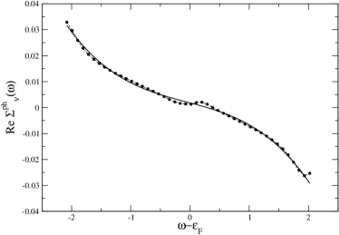
Figure 9: Real part of the phonon self-energy ${\rm Re}\Sigma_{\nu}^{ph}(\omega)$ relative to the state $\nu$ at the Fermi surface (dots), as a function of $\omega-\epsilon_{F}$ being $\epsilon_{F}$ the Fermi energy, at $\lambda=0.2$. The continuous line is the polynomial curve used to take the derivative and calculate $Z_{\nu}$.

For $\lambda=0.2$ and $\lambda=0.4$ the value of $Z_{\nu}$ about the Fermi surface has shown a very weak dependence on the degree of the polynomial chosen for the interpolation (cf. also Ref. [34]). It is remarkable that the function ${\rm Re}\Sigma_{\nu}^{ph}(\omega)$ also has a very weak dependence on $\nu$. The one reproduced in Fig. 9 very closely resembles those evaluated for different values of $\nu$. Since the staggering increases in size as one moves away from the Fermi surface, both the interpolation and the derivative become more and more ill-defined. However the contribution of these levels to the gap equation is negligible, for this reason the procedure used has demonstrated to be solid and so has the calculated value of $T_{c}$. For $\lambda=0.6$ on the other hand the staggering is large also at the Fermi surface. This once again points at the fact that the approximation used may not be entirely applicable for this interaction strength.

We now turn to discuss the effects on $T_{c}$. In Fig. 12 we show the results for $T_{c}$ as a function of $\lambda$. The two curves correspond to $T_{c}$ as evaluated using the bare interaction alone (dashed curve), and including all quasi-particle renormalization effects (solid curve).

General features - In Table 2 we report the results of the calculations when the specific effects of each renormalized quasi-particle property is isolated. The effects of the self-energy renormalizations are analogous to those we dealt with in the uniform case. The real part ${\rm Re}\Sigma^{ph}$ causes an increase in the critical temperature since, as before, it leads to an effective increase of the density of levels at the Fermi energy. On the other hand, both $Z_{\nu}$ and $\gamma_{\nu}$ depress the value of $T_{c}$, the former by causing a weaker effective interaction between quasi-particles and the latter by inhibiting pairing between quasi-particles [29].

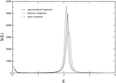
Figure 14: The figure shows the strength functions for density and spin modes with multipolarity $L=2$, for a system of 1000 particles in a sperically symmetric harmonic trap and interaction strength $\lambda=0.2$. The solid line shows the strength functions calculated with the Hartree-Fock correlation function $\Pi^{hf}$, in this case density and spin response coincide. In the RPA the two responses and distinct and are given by the dashed line and dot-dashed line respectively. The energy on the $x$-axis is measured in units of the oscillator level spacing $\hbar\omega_{0}$.

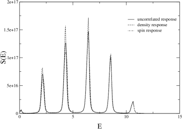
Figure 15: Same as Fig. 14 for the $L=12$ mode.

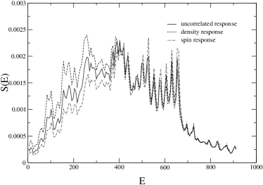
Figure 19: Same as Fig. 18 for $L=12$.

Specific features - In the weak coupling regime $\lambda=0.2$ the critical temperature is hardly affected by the renormalization of the quasi-particle properties. While this is expected as far as $\gamma_{\nu}$, $Z_{\nu}$ and ${\rm Re}\Sigma_{\nu}^{ph}$ are concerned, it is instead surprising as regards the effect of the induced interaction. For a uniform system at $\lambda=0.2$ we have seen that, if the induced interaction is calculated using only $\Pi_{\rho}^{0}$ one finds a decrease in $T_{c}$ by a factor of the order of 2. This effect is reduced, but still present, when the collectivity of the modes is accounted for. Almost no reduction is obtained instead for a trapped gas, whether one uses the lowest-order correlation function $\Pi_{\rho}^{0}$ or one accounts for the full collectivity of the modes. The absence of the reduction descends here from the discrete level structure of the harmonic trap. This can be understood by comparing the strength functions of a uniform system with those of a harmonically trapped one for the same interaction strength, see Figs. 14, 15, 18 and 19. The largest contributions to the sum in Eq. (2.4) comes from the condition $\epsilon_{\nu}=\epsilon_{\nu^{\prime}}=\omega=0$, which corresponds to particles at the Fermi surface and to the exchange of a phonon with zero frequency. The discrete level structure causes the values of the strength functions to be negligible near $\omega=0$, and consequently the effect of the phonon-induced interaction to be small. As the strength of the interaction increases ($\lambda=0.4$ and $\lambda=0.6$) the renormalization of the quasi-particle properties has a larger and larger effect on $T_{c}$. All the terms are increasingly more important but it is the quasi-particle width that dominates over the others, as can be seen in Table 2. We recall however that the case $\lambda=0.6$ is beyond the validity of the one pole approximation.

• 	$\lambda$=0.2	$\lambda$=0.4	$\lambda$=0.6
  $V^{eff}$	0.92	0.86	0.90
  $g$+ Re$\Sigma^{ph}$	1.01	1.03	1.03
  $g$+ Z	0.98	0.90	0.93
  $g$+ $\gamma$	0.97	0.85	0.76
  $V^{eff}$+ Re$\Sigma^{ph}$ + $\gamma$ + Z	0.88	0.66	0.61

Table 2: The table gives the ratio $T_{c}/T_{c}^{\rm bare}$ associated with the indicated contribution for the case of a spherically symmetric harmonic potential. $T_{c}^{\rm bare}$ is calculated including only $g$ and we find the following results: for $\lambda=0.2$, $k_{B}T_{c}^{\rm bare}=5.03\times 10^{-2}\hbar\omega_{0}$, for $\lambda=0.4$, $k_{B}T_{c}^{\rm bare}=0.34\hbar\omega_{0}$ and for $\lambda=0.6$, $k_{B}T_{c}^{\rm bare}=0.75\hbar\omega_{0}$.

Figure 10: The width $\gamma_{\nu}$ of the level $\nu$ is plotted as a function of the hartree energy $\xi_{\nu}$ for a spherically symmetric harmonic trap. The three curves correspond to the interaction strengths $\lambda=0.2$ (solid line), $\lambda=0.4$ (dashed line) and $\lambda=0.6$ (dot-dashed line). The energies are measured in units of $\hbar\omega_{0}$, with $\omega_{0}$ being the oscillator frequency.

Figure 11: The figure shows the real part of the self-energy ${\rm Re}\Sigma_{\nu}^{ph}(\epsilon_{\nu})$ of the level $\nu$ as a function of the hartree quasi-particle energy $\xi_{\nu}$ for a spherically symmetric harmonic trap. The three curves correspond to the same interaction strengths as in Fig. 10 and the same line codes and energy units are used.

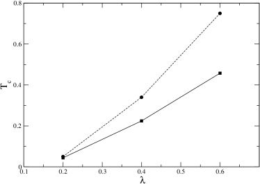
Figure 12: Critical temperature of a gas of $1000$ particles in a spherically symmetric harmonic oscillator. $T_{c}$ is in units of $\hbar\omega_{0}$. The dashed curve corresponds to $T_{c}$ calculated using the bare interaction alone, the solid one is obtained including all quasi-particle renormalization effects.

Figure 13: Critical temperature of the harmonically trapped gas with $\lambda=0.2$, as calculated from Eq. (44) including only the effective interaction contribution, as a function of the maximum multipolarity $L$ included in the correlation functions appearing in the matrix elements in Eq. (2.2). $L=1$ corresponds to the bare interaction alone. Convergence is reached around $L=27$. $T_{c}$ is in units $\hbar\omega_{0}$, with $\omega_{0}$ being the trap frequency. Circles represent the result of the calculation which includes the full induced interaction. Squares are obtained accounting only for the exchange of density modes and triangles only accounting for spin modes.

4 Conclusions

In this paper we have calculated the renormalization of the quasi-particle properties in an interacting Fermi gas due to the emission and reabsorption of density and spin fluctuations of the system. In particular we have looked, within the one pole approximation, at self-energy ($\Sigma$) and screened interaction ($V^{eff}$) effects. The real part of $\Sigma$ leads to a shift in the energy of the quasi-particles and to a reduction in the strength of the quasi-particle peak of the associated propagator (by a factor $Z\leq 1$). At the same time a non-vanishing imaginary part of $\Sigma$ results in a non-vanishing width $\gamma$ of the levels, or equivalently in a finite lifetime of the quasi-particles. The exchange of collective modes between quasi-particles leads to an effective interaction which has an overall repulsive character. This is due to the dominance of the spin triplet (repulsive) modes over spin singlet (attractive) modes, and leads to a screening of the bare attractive interaction.

Finally we have calculated the effect of these properties on the critical temperature to the superfluid state. The calculations were carried out numerically for the two illustrative cases of an isotropic infinite square well and for a harmonic trap. In both cases the calculations were carried out for a sytem of 1000 particles. We have included selectively one or the other of the renormalized quasi-particle properties and found that these have different consequences of $T_{c}$. When all of them are accounted for, the overall effect is a reduction of $T_{c}$ which depends both on the strength of the interaction and on the geometry of the system. The results are reported in Sec. 3. As the strength of the interaction increases, although the one pole approximation becomes less and less reliable, our calculations clearly indicate that the effect of fluctuations becomes more and more important and modifies the critical temperature, as compared to the one obtained using the bare quasi-particle properties, in an important way. This result is very relevant for current experiments with atomic Fermi gases. In particular it shows that the standard theories of the crossover from BCS to BEC, which are currently used to predict the value of the critical temperature also in the strongly interacting regime may be wrong by a significant amount as the interaction becomes stronger. Our approach is well suited to calculate the first corrections to the quasi-particle properties and to the critical temperature which arise when one moves towards the strongly interacting regime originating from the BCS weak coupling side.

Appendix

A.1 The correlation functions

Define:

$$\Pi_{\alpha\beta}(x,x^{\prime})=-e^{\beta\Omega}{\rm Tr}\big{\{}\hat{\rho}\;T_{\tau}[\tilde{n}_{\alpha}(x)\tilde{n}_{\beta}(x^{\prime})]\big{\}}$$

where $\tilde{n}_{\sigma}(x)=\hat{n}_{\sigma}(x)-\langle\hat{\psi}^{\dagger}_{\sigma}({{\bf r}})\hat{\psi}_{\sigma}({{\bf r}})\rangle$, with $\hat{n}_{\sigma}(x)=\hat{\psi}^{\dagger}_{\sigma}({x})\hat{\psi}_{\sigma}({x})$ and $x\equiv({\bf r},\tau)$. The indices $\alpha$, $\beta$ and $\sigma$ can assume the two values $\uparrow$ and $\downarrow$, the operator $\hat{\rho}$ is given by $\hat{\rho}=\exp[\hat{H}-\mu\hat{N}]$, with $\hat{N}=\sum_{\sigma}\int d^{3}r\;\hat{\psi}^{\dagger}_{\sigma}({{\bf r}})\hat{\psi}_{\sigma}({{\bf r}})$ and $T_{\tau}$ is the ordering operator relative to the imaginary time $\tau$. Finally $\exp(-\beta\Omega)$ is the grand partition function of the system, and $\Omega$ the thermodynamic potential.

Density correlation function - Let us now introduce the density correlation function with the definition:

$$\Pi_{\rho}(x,x^{\prime})=-e^{\beta\Omega}{\rm Tr}\big{\{}\hat{\rho}\;T_{\tau}[\tilde{n}(x)\tilde{n}(x^{\prime})]\big{\}}$$ (50)

where $\tilde{n}=\tilde{n}_{\uparrow}+\tilde{n}_{\downarrow}$. This correlation function is related to the previously defined $\Pi_{\alpha\beta}$ as follows:

$$\Pi_{\rho}(x,x^{\prime})=2\Pi_{\uparrow\uparrow}(x,x^{\prime})+2\Pi_{\uparrow\downarrow}(x,x^{\prime}),$$ (51)

where we have used $\Pi_{\uparrow\uparrow}(x,x^{\prime})=\Pi_{\downarrow\downarrow}(x,x^{\prime})$ and $\Pi_{\uparrow\downarrow}(x,x^{\prime})=\Pi_{\downarrow\uparrow}(x,x^{\prime})$.

Spin correlation function - The spin correlation function has components along the three directions $x$, $y$ and $z$, defined as follows:

$$\Pi_{\sigma_{i}}(x,x^{\prime})-e^{\beta\Omega}{\rm Tr}\big{\{}\hat{\rho}\;T_{\tau}[\hat{\sigma}_{i}(x)\hat{\sigma}_{i}(x^{\prime})]\big{\}}$$ (52)

where $\hat{\sigma}_{i}=\sum_{\alpha\beta}\hat{\psi}^{\dagger}_{\alpha}({x})(\sigma_{i})_{\alpha\beta}\hat{\psi}_{\beta}({x})$, and $(\sigma_{i})_{\alpha\beta}$ being the Pauli spin matrix element. The spin correlation function in the $z$ direction is related to $\Pi_{\alpha\beta}$ by:

$$\Pi_{\sigma_{z}}(x,x^{\prime})=2\Pi_{\uparrow\uparrow}(x,x^{\prime})-2\Pi_{\uparrow\downarrow}(x,x^{\prime}).$$ (53)

Finally since the choice of the orientation of the axes is arbitrary we must also have $\Pi_{\sigma_{x}}(x,x^{\prime})=\Pi_{\sigma_{y}}(x,x^{\prime})=\Pi_{\sigma_{z}}(x,x^{\prime})$. The $\Pi_{\alpha\beta}$ therefore contains all the information needed.

$\Pi_{\alpha\beta}$ admits the Lehmann representation:

$$\Pi_{\alpha\beta}({\bf r},{\bf r}^{\prime},i\omega_{n})=e^{\beta\Omega}(e^{-\beta E_{n}}-e^{-\beta E_{m}})\sum_{n,m\neq 0}\displaystyle\frac{\langle\Phi_{m}|\tilde{n}_{\alpha}({\bf r})|\Phi_{n}\rangle\langle\Phi_{n}|\tilde{n}_{\beta}({\bf r}^{\prime})|\Phi_{m}\rangle}{i\omega_{m}-(E_{n}-E_{m})}$$

where the complete basis of eigenstates $|\Phi_{n}\rangle$ introduced above is in principle the exact basis of excited states of the system. Below we shall assume specific approximations for the $|\Phi_{n}\rangle$’s.

A.2 The RPA approximation

To evaluate $\Pi_{\alpha\beta}$ one has to introduce specific approximations. The lowest order approximation is the Hartree-Fock particle-hole one, in which case:

$$\Pi_{\alpha\beta}^{hf}({\bf r},{\bf r}^{\prime},i\omega_{n})=\left(\begin{array}[]{cc}\chi_{0}({\bf r},{\bf r}^{\prime},i\omega_{n})&0\\ 0&\chi_{0}({\bf r},{\bf r}^{\prime},i\omega_{n})\end{array}\right).$$ (54)

As is well known a better approximation for $\Pi_{\alpha\beta}$ is the RPA self-consistent one. In this other case $\Pi_{\alpha\beta}$ is assumed to satisfy the equation (for each given $i\omega_{n}$):

$$\left(\begin{array}[]{cc}\Pi_{\uparrow\uparrow}^{r}({\bf r},{\bf r}^{\prime})&\Pi_{\uparrow\downarrow}^{r}({\bf r},{\bf r}^{\prime})\\ \Pi_{\downarrow\uparrow}^{r}({\bf r},{\bf r}^{\prime})&\Pi_{\downarrow\downarrow}^{r}({\bf r},{\bf r}^{\prime})\end{array}\right)\left(\begin{array}[]{cc}\chi_{0}({\bf r},{\bf r}^{\prime})&0\\ 0&\chi_{0}({\bf r},{\bf r}^{\prime})\end{array}\right)$$ (59)

$$+\int d^{3}r_{1}d^{3}r_{2}\;\left(\begin{array}[]{cc}\chi_{0}({\bf r},{\bf r}_{1})&0\\ 0&\chi_{0}({\bf r},{\bf r}_{1})\end{array}\right)$$ (62)

$$\left(\begin{array}[]{cc}0&g\delta({\bf r}_{1}-{\bf r}_{2})\\ g\delta({\bf r}_{1},{\bf r}_{2})&0\end{array}\right)\left(\begin{array}[]{cc}\Pi_{\uparrow\uparrow}^{r}({\bf r}_{2},{\bf r}^{\prime})&\Pi_{\uparrow\downarrow}^{r}({\bf r}_{2},{\bf r}^{\prime})\\ \Pi_{\downarrow\uparrow}^{r}({\bf r}_{2},{\bf r}^{\prime})&\Pi_{\downarrow\downarrow}^{r}({\bf r}_{2},{\bf r}^{\prime})\end{array}\right).$$ (67)

In compact notation one can write $\Pi_{\uparrow\uparrow}^{r}=\Pi_{\downarrow\downarrow}^{r}=\chi_{0}+g^{2}\chi_{0}^{3}+...$ and $\Pi_{\uparrow\downarrow}^{r}=\Pi_{\downarrow\uparrow}^{r}=g\chi_{0}^{2}+g^{3}\chi_{0}^{4}+...$ Consequently $\Pi_{\rho}^{r}=2\chi_{0}/[1-g\chi_{0}]$ and $\Pi_{\sigma_{z}}^{r}=2\chi_{0}/[1+g\chi_{0}]$.

A.3 Multipolar expansion

The spherical symmetry of our system allows expansion in multipoles:

$$\Pi_{\alpha\beta}({\bf r},{\bf r}^{\prime})=\sum_{LM}[\Pi_{\alpha\beta}(r,r^{\prime})]_{L}Y_{LM}(\Omega)Y_{LM}^{*}(\Omega^{\prime})$$ (68)

where $\Omega$ and $\Omega^{\prime}$ are the angular coordinates of ${\bf r}$ and ${\bf r}^{\prime}$ respectively.

A.4 Strength function and sum rules

Figure 16: Same as Fig. 14 for the interaction $\lambda=0.4$.

Figure 17: Same as Fig. 14 for the $L=12$ mode and interaction $\lambda=0.4$.

Figure 18: Strength function of the $L=2$ mode for a fermi gas in an isotropic infinite square well of radius $R$. The energy is in units of $\hbar^{2}/2mR^{2}$. The line codes are the same as for the previous figures.

An essential tool to study the collective modes is the strength function. This is defined as

$$S(F,E)=e^{\beta\Omega}\displaystyle\sum_{nm}(e^{-\beta E_{n}}-e^{-\beta E_{m}})$$

$$\times|\langle m|\hat{F}|n\rangle|^{2}\delta(E-E_{nm}),$$ (69)

where $\hat{F}=\sum_{\sigma}\int d^{3}rF_{\sigma}({\bf r})\hat{\psi}^{\dagger}_{\sigma}({\bf r})\hat{\psi}_{\sigma}({\bf r})$ is the operator which corresponds to external fields $F_{\uparrow}({\bf r})$ acting on the $\uparrow$ particles and $F_{\downarrow}({\bf r})$ acting on the $\downarrow$ ones. $E_{nm}$ stands for $E_{n}-E_{m}$.

The strength function is related to the retarded density correlation function by

$$S(F,E)=-\displaystyle\frac{1}{\pi}\sum_{\sigma\sigma^{\prime}}\int d^{3}r\,d^{3}r^{\prime}\,F^{*}_{\sigma}({\bf r})F_{\sigma^{\prime}}({\bf r}^{\prime}){\rm Im}\{\Pi^{0}_{\sigma\sigma^{\prime}}({\bf r},{\bf r}^{\prime},E)\}.$$

Density modes (i.e. with spin $s=0$) are excited by external fields such that $F_{\uparrow}({\bf r})=F_{\downarrow}({\bf r})$, while spin modes (with $s=1,s_{z}=0$) are excited by fields with $F_{\uparrow}({\bf r})=-F_{\downarrow}({\bf r})$.

In the particular case of a density mode of given multipolarity $L$, for which $F_{\uparrow}({\bf r})=F_{\downarrow}({\bf r})=r^{L}Y_{LM}(\Omega)$, upon use of Eq. (68), this becomes

$$S_{L}(E)=-\displaystyle\frac{1}{\pi}\sum_{\sigma\sigma^{\prime}}\int dr\,dr^{\prime}\,r^{L+2}{r^{\prime}}^{L+2}{\rm Im}\{[\Pi^{0}_{\sigma\sigma^{\prime}}(r,r^{\prime},E)]_{L}\}.$$

Also useful is the energy weighted sum-rule [33]

$$\int dE\;S(F,E)\,E=\frac{\hbar^{2}}{2m}\sum_{\sigma}\int d^{3}r\left|\nabla F_{\sigma}({\bf r})\right|^{2}n_{\sigma}(r)$$ (70)

When $F({\bf r})=r^{L}Y_{LM}(\Omega)$ it takes the simple form

$$\int dE\;S_{L}(E)E =-\displaystyle\frac{1}{\pi}\sum_{\sigma\sigma^{\prime}}\int dr\,dr^{\prime}\,r^{L+2}{r^{\prime}}^{L+2}\times{\rm Im}\{[\Pi^{0}_{\sigma\sigma^{\prime}}(r,r^{\prime},E)]_{L}\}$$ (71)

$$=\displaystyle\frac{\hbar^{2}}{2m}L(2L+1)\int_{0}^{\infty}dr\;r^{2L}n_{\sigma}(r).$$

and can be used as a check for the numerical calculations.

References

References

- [1] Jochim S, Bartenstein M, Altmeyer A, Hendl G, Riedl S, Chin C, Denschlag J H and Grimm R 2003 Science 302 2101
- [2] Greiner M, Regal C A and Jin D S 2003 Nature 426 537
- [3] Zwierlein M W, Stan C A, Schunck C H, Raupach S M F, Gupta S, Hadzibabic Z and Ketterle W 2003 Phys. Rev. Lett. 91 250401
- [4] Bourdel T, Khaykovich L, Cubizolles J, Zhang J, Chevy F, Teichmann M, Tarruell L, Kokkelmans S J J M F and Salomon C (2004) Phys. Rev. Lett. 93 050401
- [5] Kinast J, Hemmer S L, Gehm M E, Turlapov A and Thomas J E 2004 Phys. Rev. Lett. 92 150402
- [6] Leggett A J 1980, in Modern Trends in the Theory of Condensed Matter (Berlin: Springer-Verlag), pp. 13–27
- [7] Nozières P and Schmitt-Rink S 1985 J. Low Temp. Phys. 59 195
- [8] Sá de Melo C A R, Randeria M and Engelbrecht J R 1993 Phys. Rev. Lett. 71 3202
- [9] Timmermans E, Furuya K, Milonni P W and Kerman A K 2001 Phys. Lett. A 285 228
- [10] Holland M, Kokkelmans S J J M F, Chiofalo M L and Walser R 2001 Phys. Rev. Lett. 87 120406
- [11] Ohashi Y and Griffin A 2002 Phys. Rev. Lett. 89 130402
- [12] Chang S Y, Carlson J, Pandharipande V R and Schmidt K E 2004 Phys. Rev. A. 70 043602
- [13] Carlson J, Chang S Y, Pandharipande V R and Schmidt K E 2003 Phys.Rev. C 68 025802
- [14] Astrakharchik G E, Boronat J, Casulleras J and Giorgini S 2004 Phys. Rev. Lett. 93 200404
- [15] Brink D and Broglia R A (in press) Nuclear Superfluidity: pairing in finite systems (Cambridge: Cambridge University Press)
- [16] Gunnarsson D 1997 Rev. Mod. Physics 69 575
- [17] Broglia R A, Colò G, Onida G and Roman H E 2004 Solid State Physics of Finite Systems: Metal Clusters, Fullerenes, Atomic Wires (Berlin/Heidelberg: Springer-Verlag)
- [18] Giorgetti L, Viverit L, Gori G, Barranco F and Vigezzi E, Broglia R A 2004 Preprint cond-mat/0404492
- [19] Mahan G D 1990 Many-Particle Physics, 2nd Ed. (New York: Plenum Press)
- [20] The Fock contribution to the self-energy vanishes due to the form of the interaction in Eq. (1).
- [21] The Random Phase Approximation is in general a convenient tool to describe the oscillations of the mean field around the equilibrium shape, see [33].
- [22] Bruun G M and Heiselberg H 2002 Phys. Rev. A 65 053407
- [23] Bruun G M 2002 Phys. Rev. A 66, 041602
- [24] Shen C, Lombardo U, Schuck P, Zuo W and Sandulescu N 2003 Phys. Rev. C 67 061302
- [25] Bohr A and Mottelson B R 1969 Nuclear Structure (New York: W. A. Benjamin)
- [26] Barranco F, Broglia R A, Gori G, Vigezzi E, Bortignon P F and Terasaki J 1999 Phys. Rev. Lett. 83 2147
- [27] Bruun G M, Castin Y, Dum R and Burnett K 1999 Eur. Phys. J. D 7 433
- [28] Bulgac A and Yu Y 2002 Phys. Rev. Lett. 88 042504
- [29] Morel P and Nozières P 1962 Phys. Rev. 126 1909
- [30] Gorkov L P and Melik-Barkhudarov T 1961 Sov. Phys. JETP 13 1018.
- [31] Heiselberg H, Pethick C J, Smith H and Viverit L 2000 Phys. Rev. Lett. 85 2418
- [32] Combescot R 1999 Phys. Rev. Lett. 83 3766
- [33] Bertsch G F and Broglia R A 1994 Oscillations in Finite Quantum Systems (Cambridge: Cambridge University Press
- [34] Mahaux C, Bortignon P F, Broglia R A and Dasso C H 1985 Phys. Rep. 120 1