Geometry and Spectrum of Casimir Forces

Abstract

We present a new approach to the Helmholtz spectrum for arbitrarily shaped boundaries and general boundary conditions. We derive the boundary induced change of the density of states in terms of the free Green’s function from which we obtain non-perturbative results for the Casimir interaction between rigid surfaces. As an example, we compute the lateral electrodynamic force between two corrugated surfaces over a wide parameter range. Universal behavior, fixed only by the largest wavelength component of the surface shape, is identified at large surface separations, complementing known short distance expansions which we also reproduce with high precision.

The famous question “Can one hear the shape of a drum?” was posed in 1966 by Kac, illustrating the problem to deduce the shape of a region from the knowledge of its resonance spectrum Kac (1966). It was answered negatively Gordon et al. (1992) but the difficulty to characterize the distribution of eigenfrequencies of the Helmholtz wave equation in arbitrary geometries remains. This is particularly highlighted by the long-lasting efforts for chaotic (quantum) billiards which are described in two dimensions also by the wave equation Cvitanović et al. (2003). The same problems occur for Casimir interactions in three dimensions Casimir (1948) which are of much recent interest Bordag et al. (2001), mainly due to the advent of improved experimental techniques yielding the force between two parallel plates Bressi et al. (2002) and between a plate and a sphere Lamoreaux (2000). Naturally, the question arises to what extent the Casimir force characterizes the shape of the interacting objects. A large body of theoretical work, including proximity and pairwise additivity approximations Bordag et al. (2001), semi-classical approaches based on Gutzwiller’s formula Gutzwiller (1971); Schaden and Spruch (1998), a multiple scattering expansion Balian and Duplantier (1978), perturbative methods Emig et al. (2003) and recently proposed approximations from classical ray optics Jaffe and Scardicchio (2004), has been used to compute Casimir forces. However, these approaches either neglect diffraction or are limited to small smooth deformations, and reliable general expressions are not known even for simple geometries. In this Letter, we present a formula for the density of states which is formulated in terms of the free Green’s function at the boundaries only. We demonstrate its applicability by computing the lateral Casimir force between two corrugated surfaces which has been studied in a recent experiment Chen et al. (2002). We find that the surface’s shape can be deduced from the force at short distances whereas at large separations universality prevails.

The electrodynamic Casimir energy of two disconnected metallic surfaces $S_{\alpha}$, $\alpha=1,2$, is determined by the change in the photon density of states (DoS) $\delta\rho(k)=\rho(k)-\rho_{0}(k)$ caused by moving the surfaces from infinity to a finite distance in vacuum where $\rho_{0}(k)$ is the DoS for infinitely separated surfaces. Thus $\delta\rho(k)$ contains neither volume terms nor single surface contributions but measures only changes in geometry by moving the surfaces rigidly. We consider the Helmholtz equation

$$(\nabla^{2}+k^{2})\phi(\mathbf{x})=0$$ (1)

for a scalar field $\phi$ in the three connected regions separated by surfaces $S_{\alpha}$ on which $\phi$ fulfills Dirichlet (for transversal magnetic modes, TM) or Neumann (for transversal electric modes, TE) boundary conditions. The total DoS $\rho(k)$ is then given by the sum of the DoS for the three isolated regions. For simplicity, we have assumed that the surface geometry allows for a separation of the electromagnetic field into TE and TM modes which is possible for a large class of geometries as, e.g., for uniaxially deformed surfaces Emig et al. (2003). For both types of modes the Casimir energy is obtained as an integral over $\delta\rho(k)$. Since the DoS is more regular along the imaginary axis, it is useful to shift the integration to that axis and to go over from a Minkowskian to a Euclidean formulation by a Wick rotation. Then the Casimir energy becomes

$$\mathcal{E}\>=\>\frac{\hbar c}{2}\int_{0}^{\infty}dq_{0}\,q_{0}\,\delta\tilde{\rho}(q_{0})\,$$ (2)

with $\delta\tilde{\rho}(q_{0})\equiv-\delta\rho(iq_{0})$. Our main general result is the trace formula

$$\delta\tilde{\rho}(q_{0})\>=\>-\frac{1}{\pi}\frac{\partial}{\partial q_{0}}\,\text{Tr}\ln\left(\mathcal{M}\mathcal{M}_{\infty}^{-1}\right)\,,$$ (3)

where the matrix operator $\mathcal{M}$ is given by the Euclidean free Green’s function $G_{0}(\mathbf{x},\mathbf{x}^{\prime};q_{0})=e^{-q_{0}|\mathbf{x}-\mathbf{x}^{\prime}|}/(4\pi|\mathbf{x}-\mathbf{x}^{\prime}|)$ evaluated at the surfaces $S_{\alpha}$ only. Explicitly, if the surfaces $S_{\alpha}$ are represented by 3D vectors $\mathbf{s}_{\alpha}(\mathbf{u})$ with 2D local coordinates $\mathbf{u}$, then $\mathcal{M}_{\alpha\beta}(\mathbf{u},\mathbf{u}^{\prime};q_{0})=G_{0}(\mathbf{s}_{\alpha}(\mathbf{u}),\mathbf{s}_{\beta}(\mathbf{u}^{\prime});q_{0})$ for Dirichlet conditions and $\mathcal{M}_{\alpha\beta}(\mathbf{u},\mathbf{u}^{\prime};q_{0})=\partial_{\mathbf{n}_{\alpha}(\mathbf{u})}\partial_{\mathbf{n}_{\beta}(\mathbf{u}^{\prime})}G_{0}(\mathbf{s}_{\alpha}(\mathbf{u}),\mathbf{s}_{\beta}(\mathbf{u}^{\prime});q_{0})$ for Neumann conditions with $\partial_{\mathbf{n}_{\alpha}}$ the surface normal derivative pointing into the region between the surfaces. The trace in Eq. (3) is performed over the 2D coordinates and the discrete surface indices. $\mathcal{M}_{\infty}^{-1}$ is the functional inverse of $\mathcal{M}$ for infinite surface separation. A formally similar formula for the Casimir DoS has been derived by Balian and Duplantier in terms of a different matrix operator which describes surface scatterings Balian and Duplantier (1978). In the spectral theory of quantum scattering an expression of the form of Eq.(3) is known as Krein-Friedel-Lloyd formula which, however, applies to the S-matrix of potential scatterers Cvitanović et al. (2003). An important advantage of Eq.(3) is that it yields directly the regularized variation of the DoS which is free of distance independent divergences which would seriously hamper any numerical evaluations. To set an example for the applicability of our trace formula to the Casimir effect in non-trivial geometries, we compute the lateral Casimir force between corrugated surfaces which is especially sensitive to geometry. For that purpose, we employ a previously developed numerical algorithm Emig (2003); Büscher and Emig (2004) which provides a fast convergent result for the trace. It is important to note that the lateral force does not arise from a change of the mean surface separation (yielding the normal force) but from a lateral shift of the boundaries, and thus requires a careful regularization of the energy.

At first, we give a brief survey of the steps which lead to Eq. (3). We consider the Gaussian action $S=\frac{1}{2}\int d^{4}X(\nabla\phi)^{2}$ in 4D Euclidean space-time to quantize the modes of the electromagnetic field in the regions which are separated by the surfaces $S_{\alpha}$ on which Dirichlet or Neumann boundary conditions hold. Path integral techniques with delta functions enforcing the boundary conditions have been used to compute the (free) energy of constrained systems Li and Kardar (1992); Emig et al. (2003). The same approach, however, can be also used to study correlations Hanke and Kardar (2002). The modified correlations $G(\mathbf{x},\mathbf{x}^{\prime};q_{0})=\langle\phi_{q_{0}}(\mathbf{x})\phi_{-q_{0}}(\mathbf{x}^{\prime})\rangle$ in the presence of boundaries can be computed exactly in the present case of a quadratic action. If $\mathbf{x}$ and $\mathbf{x}^{\prime}$ denote two positions which are located both in the same region, one finds

$$G(\mathbf{x},\mathbf{x}^{\prime};\!q_{0})\!\! - \!\!G_{0}(\mathbf{x},\mathbf{x}^{\prime};\!q_{0})\!=\!-\!\!\sum_{\alpha\beta}\!\int\!\!d\mathbf{u}\,d\mathbf{u}^{\prime}\,G_{0}(\mathbf{x},\mathbf{s}_{\alpha}(\mathbf{u});\!q_{0})$$ (4)

$$\times \mathcal{M}^{-1}_{\alpha\beta}(\mathbf{u},\mathbf{u}^{\prime};\!q_{0})\,G_{0}(\mathbf{x}^{\prime},\mathbf{s}_{\beta}(\mathbf{u}^{\prime});\!q_{0})\,,$$

where $G_{0}$ is Green’s function in unbounded space. $\mathcal{M}^{-1}$ is the functional inverse, taken with respect to $\mathbf{u}$, $\mathbf{u}^{\prime}$ and $\alpha$, $\beta$, of the operator $\mathcal{M}$ defined after Eq. (3), see above. For a fixed region, the DoS on the imaginary axis is related to the Euclidean Green’s function by $\rho(iq_{0})=(2q_{0}/\pi)\int d^{3}\mathbf{x}\,G(\mathbf{x},\mathbf{x};q_{0})$ where the integration extends over the given region. We are actually interested in the sum of the DoS’s of the three regions into which free space is divided by the surfaces with the bulk contribution subtracted. Since Eq. (4) holds for every region, we obtain the change $\delta\rho(iq_{0})$ by integrating the r.h.s. of Eq. (4) with $\mathbf{x}^{\prime}=\mathbf{x}$ over unbounded space. Explicit integration is enabled by the simple form of Eq. (4) with $\mathbf{x}$ occurring only in the free Green’s function. Performing the integration both with $\mathcal{M}$ and $\mathcal{M}_{\infty}$ and taking the difference of the two results, we obtain Eq. (3).

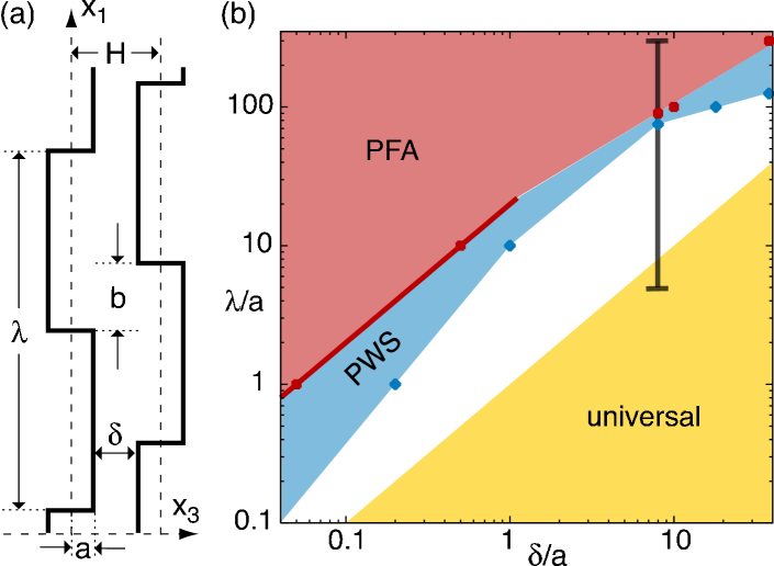
Figure 1: (a) Geometry consisting of two parallel plates with laterally shifted uniaxial rectangular gratings. (b) Approximate validity ranges of proximity force (PFA) and pairwise (PWS) approximations and sector of asymptotic universality for the lateral Casimir force as estimated from Figs.2 and 4.

In the following, we consider the geometry depicted in Fig. 1(a). It consists of two surfaces with uniaxial rectangular gratings along the $x_{1}$ axis with equal amplitude $a$ and wavelength $\lambda$. The surfaces are laterally shifted by $b$ and have a mean separation $H$, yielding a minimal gap $\delta=H-2a$. The Casimir energy of these surfaces at fixed $H$ has to be a periodic function of $b$, and it should be minimal if the surface area with minimal surface distance is maximal, i.e., for $b=\lambda$. This leads to a lateral force $F_{\rm lat}=-\partial\mathcal{E}/\partial b$. Performing the frequency integration by parts in Eq. (2) with Eq. (3), we find

$$F_{\rm lat}=-\frac{\hbar c}{2\pi}\int_{0}^{\infty}\!\!\!dq_{0}\,{\rm Tr}\left(\mathcal{M}^{-1}\partial_{b}\mathcal{M}-\mathcal{M}_{\infty}^{-1}\partial_{b}\mathcal{M}_{\infty}\right)\,.$$ (5)

For periodic geometries as the one considered here, the trace can be computed with the technique introduced in Emig (2003); Büscher and Emig (2004). We Fourier transform $\mathcal{M}_{\alpha\beta}(\mathbf{u},\mathbf{u}^{\prime};q_{0})$ with respect to $\mathbf{u}$ and $\mathbf{u}^{\prime}$ so that use can made of the periodicity along $x_{1}$ and translational invariance along $x_{2}$, allowing for the representation

$$\begin{split}&\tilde{\mathcal{M}}_{\alpha\beta}\left(\mathbf{p},\mathbf{q};q_{0}\right)\>=\>(2\pi)^{2}\delta\left(p_{2}+q_{2}\right)\\ &\times\sum_{m=-\infty}^{\infty}\delta\left(p_{1}+q_{1}+2\pi m/\lambda\right)\,N_{m}^{\alpha\beta}\left(q_{1},q_{2};q_{0}\right)\,,\end{split}$$ (6)

which defines the $2\times 2$ matrices $N_{m}$ that can be computed analytically and are given in Büscher and Emig (2004) for the geometry of Fig.1(a). The trace in Eq.(5) is more efficiently obtained if it is restricted to momenta $q_{1}$ in the interval $[0,2\pi/\lambda)$. This is possible after a rearrangement of the elements of $\tilde{\mathcal{M}}$ so that it has block-diagonal form where the blocks are numbered by the continuous index $q_{1}$ in $[0,2\pi/\lambda)$ and, for fixed $q_{0}$, $q_{2}$, have matrix elements $B_{kl}^{\alpha\beta}(q_{1},q_{2};q_{0})=N_{k-l}^{\alpha\beta}(q_{1}+2\pi l/\lambda,q_{2};q_{0})$ for integer indices $k$, $l=-\infty,\ldots,\infty$. Physically, a block with index $q_{1}$ couples only waves whose momenta differ from the Bloch momentum $q_{1}$ by integer multiples of $2\pi/\lambda$. Thus, in analogy to Bloch’s theorem, the original problem has separated into decoupled subproblems at a fixed $q_{1}$ in the interval $[0,2\pi/\lambda)$, and the total trace in Eq.(5) is given by the sum over the traces of the subproblems. This fact can be expressed by defining the function $g(q_{1},q_{2};q_{0})=\text{tr}(B^{-1}\partial_{b}B-B^{-1}_{\infty}\partial_{b}B_{\infty})$ where the trace runs over the indices $k$, $l$, $\alpha$, $\beta$ of $B$, and $B_{\infty}$ is the analog of $\mathcal{M}_{\infty}$, i.e., $B$ for $H\to\infty$. The lateral Casimir force is then given by

$$F_{\rm lat}=-\frac{\hbar c}{8\pi^{2}}\int_{0}^{\infty}\!dq\,q\int_{0}^{2\pi/\lambda}\!dq_{1}\,g(q_{1},q_{2};q_{0})\,,$$ (7)

with $q=\sqrt{q_{0}^{2}+q_{2}^{2}}$. Since the matrices $N_{m}$ are known analytically Büscher and Emig (2004), the same applies to $B$, $B_{\infty}$, and the derivative with respect to $b$ can be easily computed. However, for a non-perturbative treatment, the inversions of $B$, $B_{\infty}$ have to be implemented numerically. This is enabled by a truncation of the matrix $B$ at a fixed order $M$ so that the function $g$ is replaced by $g_{M}$ which is defined as $g$ above but with the trace running over $k,l=-M\dots M$ only. $F_{\rm lat}$ follows then from a numerical integration over $g_{M}$ in Eq. (7) for a sequence of fixed $M$ and a subsequent extrapolation to $M\to\infty$. For the results shown below, we have chosen $M$ between $13$ and $37$ with the larger $M$ used at smaller separations $\delta$. This is physically consistent with the fact that with increasing separation smaller integer multiples of $2\pi/\lambda$ around the Bloch momenta have to be considered. It should be stressed that the above analysis is independent of the boundary conditions which, however, change $\mathcal{M}$. Thus the electromagnetic Casimir force is the sum of $F_{\rm lat}$ for Dirichlet and Neumann boundary conditions, respectively, leading to the results for $F_{\rm lat}$ summarized in Figs. 2-3.

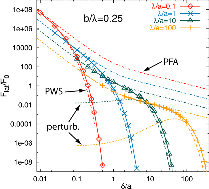
Figure 2: Lateral force $F_{\rm lat}$ at $b=\lambda/4$ obtained from Eq. (7) for the geometry of Fig. 1(a) as function of the surface gap $\delta$ (solid curves). $F_{\rm lat}$ is measured in units of the normal force $F_{0}$ between flat surfaces with $a=0$. Plotted are also the proximity force (PFA, dash-dotted curves) and pairwise summation (PWS, dashed curves) approximations, and the perturbative result $F_{\rm pt}$ for sinusoidal profiles (dotted curves) Emig et al. (2003).

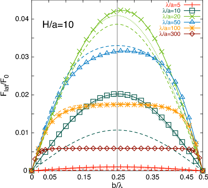
Figure 3: Shape dependence of $F_{\rm lat}$ on the lateral surface shift $b$ at fixed distance $H=10a$ for different corrugation lengths. The dashed and the dotted curves represent the PWS and the full perturbative result for sinusoidal profiles with arbitrary $H/\lambda$ Emig et al. (2003), respectively.

At short surface distances approximative methods can be employed and it is instructive to compare their predictions to our findings. To begin with, the proximity force approximation Bordag et al. (2001) yields the lateral force $F_{\rm PFA}=[2\mathcal{E}_{0}(H)-\mathcal{E}_{0}(H-2a)-\mathcal{E}_{0}(H+2a)]/\lambda$ for $0<b<\lambda/2$ with $\mathcal{E}_{0}(H)=-(\pi^{2}/720)\hbar c/H^{3}$ since it sums the flat plate energy $\mathcal{E}_{0}$ at the local distance normal to the surfaces. $F_{\rm PFA}$ changes sign at $b=\lambda/2$ discontinuously. A different approximation consists in the pairwise summation (PWS) of Casimir-Polder potentials. Although strictly justified for rarefied media only, it is often also applied to metals, using the two-body potential $U(r)=-(\pi/24)\hbar c/r^{7}$ whose amplitude is chosen as to reproduce the correct result for flat ideal metal plates Bordag et al. (2001). It yields the lateral force $F_{\rm PWS}=-\frac{\partial}{\partial b}\int_{V_{l}}d^{3}\mathbf{x}\int_{V_{r}}d^{3}\mathbf{x}^{\prime}U(|\mathbf{x}-\mathbf{x}^{\prime}|)$ with $V_{l}$ and $V_{r}$ denoting the semi-infinite regions to the left and right of the two surfaces in Fig.1(a), respectively. To compute $F_{\rm PWS}$, we have first differentiated analytically with respect to $b$ and then performed the remaining integrals numerically. Fig.2 shows our results for the amplitude of the lateral force, measured relative to the normal force $F_{0}$ between flat plates at the same $H$, over more than 4 orders of magnitude for the gap $\delta$ together with the two approximations. For small $\delta$, both approximations agree and match our results. Beyond $\delta\gtrsim\lambda/20$ the PFA starts to fail since it does not capture the exponential decay of $F_{\rm lat}$ for increasing $\delta$. The PWS approach has a slightly larger validity range [cf. Fig.1(b)] and reproduces the exponential decay. However it deviates by at least one order of magnitude from $F_{\rm lat}$ for $\delta\gtrsim 2.5\lambda$, see Fig.2. Thus it is important that in the asymptotic limit of large surface gaps, one can expect a universal behavior of the force which is independent of the detailed shape of the surface corrugation. Precisely this expectation is strikingly confirmed when we compare our results to the perturbative expression for the lateral force for sinusoidally shaped surfaces (with amplitude $a_{0}$ and wavelength $\lambda$) Emig et al. (2003),

$$F_{\rm pt}=\frac{8\pi^{3}\,\hbar c}{15}\frac{a_{0}^{2}}{\lambda^{5}H}\,\sin\left(\frac{2\pi}{\lambda}\,b\right)e^{-2\pi H/\lambda}\,,$$ (8)

which is expected to hold for $a_{0}\ll\lambda\ll H$. By considering the lowest harmonic of the rectangular corrugation, which corresponds in Eq.(8) to $a_{0}=4a/\pi$, we find excellent agreement between $F_{\rm pt}$ and our results for the geometry of Fig.1(a) for large distances $\delta\gtrsim\lambda$, see Fig.2. Higher harmonics describing short scale surface structure are irrelevant for the asymptotic Casimir interaction. This is particularly highlighted by the dependence of the force on the lateral shift $b$ shown in Fig.3 for $H=10a$ and $\lambda$ varying in the interval indicated by the bar in Fig.1(b). With changing $\lambda$, three regimes can be identified. For $\lambda\gg H$, the force profile resembles almost the rectangular shape of the surfaces, and the PWS approach yields consistent results. For decreasing $\lambda$, yet larger than $H$, the force profile becomes asymmetric with respect to $b=\lambda/4$ and more peaked, signaling the crossover to the universal regime for $\lambda\lesssim H$ where the force profile is sinusoidal. In the latter case, for not too small $\lambda/a\approx 10$, our results for $F_{\rm lat}$ indeed agree well with the perturbative result for arbitrary $H/\lambda$ of Ref.Emig et al. (2003), cf. Fig.3. We note that the PWS approach fails to predict the asymmetry of the force profile, and the PFA even predicts no variation at all with $b$ in the range of Fig.3. Finally, we observe a non-monotonous change of the lateral force with $H/\lambda$ when $H/a$ is kept fixed, see Fig.4. After a linear increase of $F_{\rm lat}/F_{0}$, described by the PFA, the force shows a maximum beyond which it decays exponentially. For small amplitudes, $a/H=1/40$ in Fig.4, the position of the maximum at $H\approx 0.4\lambda$ is again in good agreement with the full perturbative result Emig et al. (2003). With increasing $a/H$, the maximum is shifted towards smaller wavelengths.

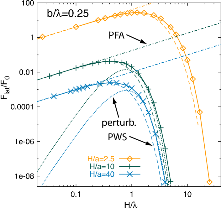
Figure 4: Dependence of $F_{\rm lat}$ (solid curves) on the corrugation length $\lambda$ at fixed mean distances $H$. Shown are also the approximations (PFA, PWS) for short distances and the perturbative result $F_{\rm pt}$ for $a\ll H$, $\lambda$.

In conclusion, we have derived a formula for the change of the Helmholtz spectrum by arbitrarily shaped boundaries. From non-perturbative results based on this formula, we argue that the lateral Casimir force between any two uniaxially corrugated surfaces of equal wavelength and amplitude is described by Eq.(8) for $H$ much larger than the wave length. We note that the validity range for this universal behavior is not fully realized in the experiment of Chen et al. (2002) with $H/a\approx 10$ and $\lambda/a\approx 55$ when $a$ is set to the geometric mean of the distinct amplitudes of the experiment. It would be interesting to probe this universality in experiments with different shapes at larger ratios $H/\lambda$. We studied surface deformations with a bounded spectrum. Stochastic surface roughness does not have this feature, and we then expect a different asymptotic behavior. We note that our approach yields also the non-integrated DoS and can be easily used in any space dimension, and also for closed boundaries. This might be of importance for applications to chaotic systems as quantum billiards. At finite temperatures, the DoS has to be integrated with a saw teeth-like weight Balian and Duplantier (1978). Finally, material properties of the surfaces can be included in our approach in form of non-local boundary conditions Emig and Büscher (2004).

This work was supported by the Deutsche Forschungsgemeinschaft through the Emmy Noether grant No. EM70/2-3.

References

- Kac (1966) M. Kac, Amer. Math. Monthly 73, 1 (1966).
- Gordon et al. (1992) C. Gordon, D. L. Webb, and S. Wolpert, Bull. Am. Math. Soc. 27, 134 (1992).
- Cvitanović et al. (2003) P. Cvitanović et al., Chaos: Classical and Quantum (Niels Bohr Institute, Copenhagen, 2003), chaosBook.org.
- Casimir (1948) H. B. G. Casimir, Proc. K. Ned. Akad. Wet. 51, 793 (1948).
- Bordag et al. (2001) M. Bordag, U. Mohideen, and V. M. Mostepanenko, Phys. Rep. 353, 1 (2001).
- Bressi et al. (2002) G. Bressi, G. Carugno, R. Onofrio, and G. Ruoso, Phys. Rev. Lett. 88, 041804 (2002).
- Lamoreaux (2000) S. K. Lamoreaux, Phys. Rev. Lett. 84, 5673 (2000).
- Gutzwiller (1971) M. C. Gutzwiller, J. Math. Phys. (N.Y.) 12, 343 (1971).
- Schaden and Spruch (1998) M. Schaden and L. Spruch, Phys. Rev. A 58, 935 (1998).
- Balian and Duplantier (1978) R. Balian and B. Duplantier, Ann. Phys. 112, 165 (1978).
- Emig et al. (2003) T. Emig, A. Hanke, R. Golestanian, and M. Kardar, Phys. Rev. Lett. 87, 260402 (2001); Phys. Rev. A 67, 022114 (2003);
- Jaffe and Scardicchio (2004) R. L. Jaffe and A. Scardicchio, Phys. Rev. Lett. 92, 070402 (2004).
- Chen et al. (2002) F. Chen, U. Mohideen, G. L. Klimchitskaya, and V. M. Mostepanenko, Phys. Rev. Lett. 88, 101801 (2002).
- Büscher and Emig (2004) R. Büscher and T. Emig, Phys. Rev. A 69, 062101 (2004).
- Emig (2003) T. Emig, Europhys. Lett. 62, 466 (2003).
- Li and Kardar (1992) H. Li and M. Kardar, Phys. Rev. A 46, 6490 (1992).
- Hanke and Kardar (2002) A. Hanke and M. Kardar, Phys. Rev. A 65, 046121 (2002).
- Emig and Büscher (2004) T. Emig and R. Büscher, Nucl. Phys. B 696, 468 (2004).