Competition and cooperation:
aspects of dynamics in sandpiles

Abstract

In this article, we review some of our approaches to granular dynamics, now well known [1] to consist of both fast and slow relaxational processes. In the first case, grains typically compete with each other, while in the second, they cooperate. A typical result of cooperation is the formation of stable bridges, signatures of spatiotemporal inhomogeneities; we review their geometrical characteristics and compare theoretical results with those of independent simulations. Cooperative excitations due to local density fluctuations are also responsible for relaxation at the angle of repose; the competition between these fluctuations and external driving forces, can, on the other hand, result in a (rare) collapse of the sandpile to the horizontal. Both these features are present in a theory reviewed here. An arena where the effects of cooperation versus competition are felt most keenly is granular compaction; we review here a random graph model, where three-spin interactions are used to model compaction under tapping. The compaction curve shows distinct regions where ’fast’ and ’slow’ dynamics apply, separated by what we have called the single-particle relaxation threshold. In the final section of this paper, we explore the effect of shape – jagged vs. regular – on the compaction of packings near their jamming limit. One of our major results is an entropic landscape that, while microscopically rough, manifests Edwards’ flatness at a macroscopic level. Another major result is that of surface intermittency under low-intensity shaking.

, , ,

1 INTRODUCTION

Matter in the jammed state has become a focus of interest for physicists in recent years.Two prime examples of this in the context of natural systems are glasses [2, 3] and densely packed granular media [4]; while the mechanisms of jamming in each case show strong similarities, the ineffectiveness of temperature as a dynamical motor in granular media leads to vastly more surprising effects. A direct consequence of such athermal behaviour in sandpiles is the stable formation of cooperative structures such as bridges [5], or indeed the very existence [6] of an angle of repose [7]; neither would be possible in the presence of Brownian motion. We discuss our studies of these two effects in the first two sections of this article. The last two sections, with their focus on jamming, unify aspects of glasses and granular media; one of them uses random graphs to illustrate competitive and cooperative effects in granular compaction [8]. The other concerns itself mainly with the fast dynamics in the boundary layer of a granular column, as the jamming limit is approached; it makes clear how asymmetric grains can orient themselves suitably so as to waste less space, when compelled so to do [9].

2 On bridges in sandpiles - an overarching scenario

The athermal nature of granular media results in the following fact: all granular dynamics is the result of external stimuli. These result in grains competing with each other to fall under gravity to a point of stability; when instead, the process is one of cooperation so that two or more grains fall together to rest on the substrate with mutual support, bridges [5] are formed. These can be stable for arbitrarily long times, since the Brownian motion that would dissolve them away in a liquid is absent in sandpiles – grains are simply too large for the ambient temperature to have any effect. As a result, bridges can affect the ensuing dynamics of the sandpile; a major mechanism of compaction is the gradual collapse of long-lived bridges in weakly vibrated granular media, resulting in the disappearance of the voids that were earlier enclosed [10]. Bridges are also responsible for jamming in granular processes, for example, as grains flow out of a hopper [6].

We first define a bridge in more quantitative terms. Consider a stable packing of hard spheres under gravity, in three dimensions. Each particle typically rests on three others which stabilise it, in the sense that downward motion is impeded. A bridge is a configuration of particles in which the three-point stability conditions of two or more particles are linked; that is, two or more particles are mutually stabilised. Bridges thus cannot be formed sequentially, but are ubiquitous in generic powders. While it is impossible to determine bridge distributions uniquely from a distribution of particle positions, we are able via our algorithm to obtain the most likely positions of bridges in a given scenario [5].

We now distinguish between linear and complex bridges via a comparison of Figures 1 and 2. Figure 1 illustrates a complex bridge, i.e., a mutually stabilised cluster of five particles (shown in green), where the stability is provided by six stable base particles (shown in blue). Of course the whole is embedded in a stable network of grains within the sandpile. Also shown is the network of contacts for the particles in the bridge: we see clearly that three of the particles each have two mutual stabilisations. Figure 2 illustrates a seven particle linear bridge with nine base particles. This is an example of a linear bridge. The contact network shows that this bridge has a simpler topology than that in Figure 1. Here, all of the mutually stabilised particles are in sequence, as in a string. A linear bridge made of $n$ particles therefore always rests on $n_{\rm b}=n+2$ base particles. For a complex bridge of size $n$, the number of base particles is reduced ($n_{\rm b}<n+2$), because of the presence of loops in their contact networks.

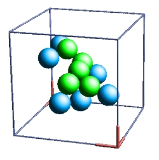
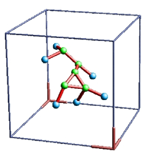
Figure 1: A five particle complex bridge, with six base particles (left), and the corresponding contact network (right). Thus $n=5$ and $n_{\rm b}=6<5+2$.

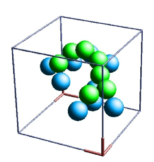
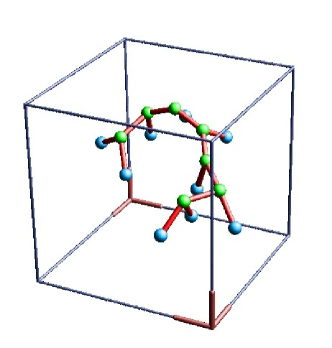
Figure 2: A seven particle linear bridge with nine base particles (left), and the corresponding contact network (right). Thus $n=7$ and $n_{\rm b}=9=7+2$.

An important point to note is that bridges can only be formed sustainably in the presence of friction; the mutual stabilisations needed would be unstable otherwise! Although our Monte Carlo simulations (described below) do not contain friction explicitly, our configurations indirectly include this: in particular, the coordination numbers lie in a range consistent with the presence of friction [10, 11, 12].

2.1 Simulation details

We have examined bridge structures in hard assemblies that are generated by a non-sequential restructuring algorithm [10], whose main modelling ingredients involve stochastic grain displacements and collective relaxation from them.

This algorithm restructures a stable hard sphere deposit in three distinct stages.

• The granular assembly is dilated in a vertical direction (with free volume being introduced homogeneously throughout the system), and each particle is given a random horizontal displacement; this models the dilation phase of a vibrated granular medium.

• The assembly is compressed in a uniaxial external field representing gravity, using a low-temperature Monte Carlo process.

• Individual spheres in the assembly are stabilised using a steepest descent ‘drop and roll’ dynamics to find local potential energy minima.

Steps (2) and (3) model the quench phase of the vibration, where particles relax to locally stable positions in the presence of gravity. Crucially, during the third phase, the spheres are able to roll in contact with others; mutual stabilisations are thus allowed to arise, mimicking collective effects. The final configuration has a well-defined contact network where each sphere is supported by a uniquely defined set of three other spheres.

The simulation method recalled above builds a sequence of static packings. Each new packing is built from its predecessor by a random process and the sequence achieves a steady state, where structural descriptors such as the mean packing fraction and the mean coordination number fluctuate about well-defined mean values. The steady-state mean volume fraction $\Phi$ typically evolves to values in the range $\Phi\sim 0.55\hbox{ -- }0.61$, depending on the shaking amplitude; the mean coordination number is always $Z\approx 4.6\pm 0.1$. We recall that for frictionless (isostatic) packings in $d$ dimensions, $Z=2d$ ($=6$ for $d=3$) [13], while for frictional packings the minimal coordination number is $Z=d+1$ ($=4$ for $d=3$) [11]; our configurations thus clearly correspond to those generated in the presence of friction. This is confirmed by the results of molecular dynamics simulations of sphere packings in the limit of high friction, which yield a mean coordination number slightly above $4.5$ [12].

Each of our configurations includes $N_{\rm tot}\approx 2200$ particles. Segregation is avoided by choosing monodisperse particles: a rough base prevents ordering. A large number of restructuring cycles is needed to reach the steady state for a given shaking amplitude: about 100 stable configurations (picked every 100 cycles in order to avoid correlation effects) are analysed, corresponding to $\Phi=0.56$ and $\Phi=0.58$. From these configurations, and following specific prescriptions, our algorithm identifies bridges as clusters of mutually stabilised particles [5].

Figure 3 illustrates two characteristic descriptors of bridges used in this work. The main axis of a bridge is defined using triangulation of its base particles as follows: triangles are constructed by choosing all possible connected triplets of base particles, and the vector sum of their normals is defined to be the direction of the main axis of the bridge. The orientation angle $\Theta$ is defined as the angle between the main axis and the $z$-axis. The base extension $b$ is defined as the radius of gyration of the base particles about the $z$-axis; note that this is distinct from the radius of gyration about the main axis of the bridge.

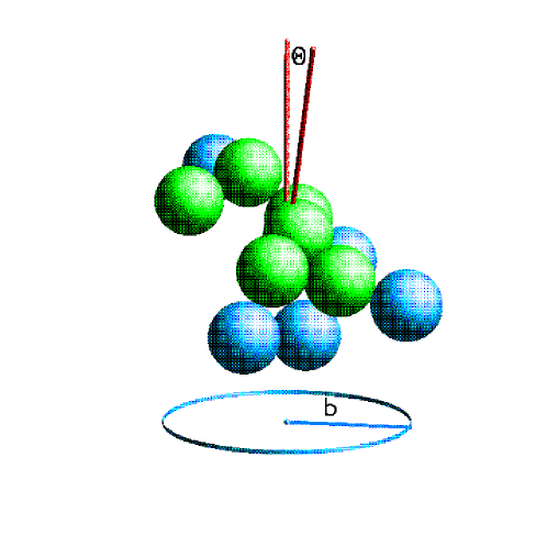
Figure 3: Definition of the angle $\Theta$ and the base extension $b$ of a bridge. The main axis makes an angle $\Theta$ with the $z$-axis; the base extension $b$ is the projection of the radius of gyration of the bridge on the $x$-$y$ plane.

2.2 Bridge sizes and diameters: when does a bridge span a hole?

In the following, we present statistics for both linear and complex bridges. While we recognise that bridge formation is a collective dynamical process, we adopt an ergodic viewpoint [14] here. Inspired by polymer theory [15], we visualise a linear bridge as a random chain which grows as a continuous curve, i.e. ’sequentially’ in terms of its arc length $s$. (For complex bridges, this simplification is not possible in general – a direct consequence of their branched structure). This replacement of what is in reality a collective phenomenon in time by a random walk in space is somewhat analogous to the ’tube model’ of linear polymers [15]: both are simple but efficient effective pictures of very complex problems.

We first address the question of the length distribution of linear bridges. We define the length distribution $f_{n}$ as the probability that a linear bridge consists of exactly $n$ spheres. We make the simplest and the most natural assumption that a bridge of size $n$ remains linear with some probability $p<1$ if an $(n+1)^{\rm th}$ sphere is ’added’ to it: this leads to the exponential distribution

$$f_{n}=(1-p)p^{n}.$$ (2.1)

The exponential distribution above can also be derived by means of a continuum approach. Here, a linear bridge is viewed as a continuous random curve or ‘string’, parametrised by the arc length $s$ from one of its endpoints. We assume also that such a bridge disappears at a constant rate $\alpha$ per unit length, either by changing from linear to complex or by collapsing. The survival probability $S(s)$ of a linear bridge upto length $s$ thus obeys the rate equation $\dot{S}=-\alpha S$ and falls off exponentially, according to $S(s)=\exp(-\alpha s)$. Consequently, the probability distribution of the length $s$ of linear bridges reads $f(s)=-\dot{S}(s)=\alpha\,\exp(-\alpha s)$, a continuum analogue of (2.1).

This is in good accord with the results of independent simulations, which exhibit an exponential decay of linear bridges of the form (2.1), with $\alpha\approx 0.99$ [5], which is clearly seen until $n\approx 12$. Around $n\approx 8$, complex bridges begin to predominate; these have size distributions which show a power-law decay:

$$f_{n}\sim n^{-\tau}.$$ (2.2)

with $\tau\approx 2$ [5].

We have also measured the diameter $R_{n}$ of linear and complex bridges of size $n$, which is such that $R_{n}^{2}$ is the mean squared end-to-end distance. Our data on diameters and size distributions [5] indicate that linear bridges in three dimensions start off as planar self-avoiding walks, which eventually collapse onto each other because of vibrational effects; on the other hand, complex bridges look like $3d$ percolation clusters.

Another issue of interest to us is the jamming potential of a bridge. A measure of this, in the case of a linear bridge, is its the base extension $b$ (see Figure 3); this is the horizontal projection of the ’span’ of the bridge. Our simulation results [5] indicate that three-dimensional bridges of a given length have a fairly characteristic horizontal extension, making it relatively easy to predict whether or not they would ’jam’ a given hole.

In order to compare our simulations with experiment [16, 17], we plot in Figure 4 the logarithm of the probability distribution of base extensions $p(b)$ against the (normalised) base extension $b/\langle b\rangle$. This figure emphasises the exponential tail of the distribution function, and also shows that bridges with small base extensions are unfavoured. We note that this long tail is characteristic of three-dimensional experiments on force chains in granular media [17]. The sharp drop at the origin as well as the long tail in Figure 4, are observed in normal force distributions obtained via molecular dynamics simulations of particle packings [18], in the limit of strong deformations. Realising that the measured forces propagate through chains of particles, we use this similarity to suggest that bridges are really just long-lived force chains, which have survived despite strong deformations. We suggest also that with the current availability of 3D visualisation techniques such as NMR [19], bridge configurations might be an easily measurable and effective tool to probe inhomogeneities in shaken sand.

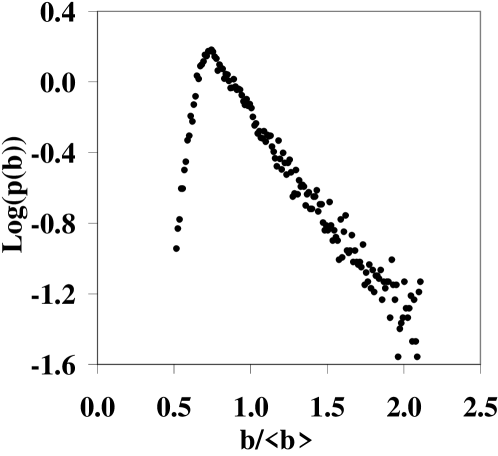
Figure 4: Distribution of base extensions of bridges, for $\Phi=0.58$. The logarithm of the normalised probability distribution is plotted as a function of the normalised variable $b/\langle b\rangle$, where $\langle b\rangle$ is the mean extension of bridge bases.

2.3 Turning over at the top; how linear bridges form domes

Recall that a linear bridge is modelled as a continuous curve, parametrised by its arc length $s$. We here focus on its most important degree of freedom, the tilt with respect to the horizontal; the azimuthal degree of freedom is neglected. Accordingly, we define the local or link angle $\theta(s)$ between the direction of the tangent to the bridge at point $s$ and the horizontal, and the mean angle made by the bridge from its origin up to point $s$, also with the horizontal:

$$\Theta(s)=\displaystyle{\displaystyle 1\over\displaystyle s}\int_{0}^{s}\theta(u)\,{\rm d}u.$$ (2.3)

The local angle $\theta(s)$ so defined may be either positive or negative; it can even change sign along the random curve which represents a linear bridge. Of course, the orientation angle $\Theta$ measured in our numerical simulations is positive by construction, being defined as the angle between the main bridge axis and the $z$-axis (see Figure 3). (Note that by simple geometry, this ’zenith angle’ made by the bridge axis with the vertical, equals the mean angle made by the basal plane of the bridge with the horizontal).

Our simulations show that the mean angle $\Theta(s)$ typically becomes smaller and smaller as the length $s$ of the bridge increases. Small linear bridges are almost never flat [5]; as they get longer, assuming that they still stay linear, they get ‘weighed down’, arching over as at the mouth of a hopper [6]. Thus, in addition to our earlier claim that long linear bridges are rare, we claim further here that (if and) when they exist, they typically have flat bases, becoming ‘domes’.

We use these insights to write down equations to investigate the angular distribution of linear bridges. These couple the evolution of the local angle $\theta(s)$ with local density fluctuations $\phi(s)$ at point $s$ (with ^′ denoting a derivative with respect to $s$):

$$\theta^{\prime}=-a\theta-b\phi^{2}+\Delta_{1}\eta_{1}(s),$$ (2.4)

$$\phi^{\prime}=-c\phi+\Delta_{2}\eta_{2}(s).$$ (2.5)

The effects of vibration on each of $\theta$ and $\phi$ are represented by two independent white noises $\eta_{1}(s)$, $\eta_{2}(s)$, such that

$$\langle\eta_{i}(s)\eta_{j}(s^{\prime})\rangle=2\,\delta_{ij}\,\delta(s-s^{\prime}),$$ (2.6)

whereas the parameters $a$, …, $\Delta_{2}$ are assumed to be constant.

The phenomenology behind the above equations is the following: the evolution of $\theta(s)$ is caused, in our effective picture, by the sequential addition of particles to the bridge at its ends. The fluctuations of local density $\phi$ at a point $s$ are caused by collective particle motion [20]. The first terms on the right-hand side of (2.4), (2.5) say that neither $\theta$ nor $\phi$ is allowed to be arbitrarily large. Their coupling via the second term in (2.4) arises as follows: if there are density fluctuations $\phi^{2}$ of large magnitude at the tip of a bridge, these will, to a first approximation, ‘weigh the bridge down’, i.e., decrease the angle $\theta$ locally.

Reasoning as above, we therefore anticipate that for low-intensity vibrations and stable bridges, both density fluctuations $\phi(s)$ and link angles $\theta(s)$ will be small. Accordingly, we linearise (2.4), obtaining thus an Ornstein-Uhlenbeck equation:

$$\theta^{\prime}=-a\theta+\Delta_{1}\eta_{1}(s).$$ (2.7)

Let us make the additional assumption that the initial angle $\theta_{0}$, i.e., that observed for very small bridges, is itself Gaussian with variance $\sigma_{0}^{2}=\langle\theta_{0}^{2}\rangle$. The angle $\theta(s)$ is then a Gaussian process with zero mean for any value of the length $s$. Its correlation function can be easily evaluated to be [21]:

$$\langle\theta(s)\theta(s^{\prime})\rangle=\sigma_{\rm eq}^{2}\,{\rm e}^{-a|s-s^{\prime}|}+(\sigma_{0}^{2}-\sigma_{\rm eq}^{2}){\rm e}^{-a(s+s^{\prime})}.$$ (2.8)

It follows from this that the variance of the link angle is:

$$\langle\theta^{2}\rangle(s)=\sigma_{\rm eq}^{2}+(\sigma_{0}^{2}-\sigma_{\rm eq}^{2}){\rm e}^{-2as},$$ (2.9)

We see from the above that orientation correlations decay with a characteristic length given by $\xi=1/a$; also, in the limit of an infinite bridge, the variance $\langle\theta^{2}\rangle$ relaxes to $\sigma_{\rm eq}^{2}=\displaystyle{\displaystyle\Delta_{1}^{2}\over\displaystyle a}$ [5]. Thus, as the chain gets longer, the variance of the link angle relaxes from its initial value of $\sigma_{0}^{2}$ (i.e. that for the initial link) to $\sigma_{\rm eq}^{2}$ for infinitely long chains.

Given the above, it can be shown that the mean angle $\Theta(s)$ will also have a Gaussian distribution. Its variance can be derived by inserting (2.8) into (2.3):

$$\langle\Theta^{2}\rangle(s)=2\sigma_{\rm eq}^{2}\,\displaystyle{\displaystyle as-1+{\rm e}^{-as}\over\displaystyle a^{2}s^{2}}+(\sigma_{0}^{2}-\sigma_{\rm eq}^{2})\displaystyle{\displaystyle(1-{\rm e}^{-as})^{2}\over\displaystyle a^{2}s^{2}}.$$ (2.10)

The asymptotic result

$$\langle\Theta^{2}\rangle(s)\approx\displaystyle{\displaystyle 2\sigma_{\rm eq}^{2}\over\displaystyle as}\approx\displaystyle{\displaystyle 2\Delta_{1}^{2}\over\displaystyle a^{2}s},$$ (2.11)

confirms our earlier statement that the longest bridges form domes, i.e. they have bases that are almost flat. Each such bridge can be viewed as consisting of a large number $as=s/\xi\gg 1$ of independent ‘blobs’ of length $\xi$; this result suggests, yet again, strong analogies between linear bridges and linear polymers [15].

The result (2.11) has another interpretation. As $\Theta(s)$ is small with high probability for a very long bridge, its extension in the vertical direction reads approximately

$$Z=z(s)-z(0)\approx s\,\Theta(s),$$ (2.12)

so that $\langle Z^{2}\rangle\approx s^{2}\langle\Theta^{2}\rangle(s)\approx 2(\Delta_{1}/a)^{2}\,s$. Switching back to a discrete picture of an $n$-link chain, we have

$$Z_{n}\sim n^{1/2}.$$ (2.13)

The vertical extension of a linear bridge is thus found to grow with the usual random-walk exponent $1/2$, in agreement with experiments on two-dimensional arches [16]. Our observations on horizontal extensions of three-dimensional bridges have yielded [5] a non-trivial exponent $\nu_{\rm lin}\approx 0.66$. Putting all of this together, our results predict that long linear bridges are domelike; also, they are vertically diffusive but horizontally superdiffusive. Evidently, jamming in a three-dimensional hopper would be caused by the planar projection of such a dome.

We now compare the results of this simple theory with data on bridge structures obtained from independent numerical simulations of shaken hard sphere packings [10]. Figure 5 confirms that the mean angle is Gaussian to a good approximation, while Figure 6 shows the measured size dependence of the variance $\langle\Theta^{2}\rangle(s)$. The numerical data are found to agree well with a common fit to the first (stationary) term of (2.10) - the ‘transient’ effects of the second term of (2.10) are too small to be significant at our present accuracy. We thus conclude that our simple theory captures the principal structural features of linear bridges.

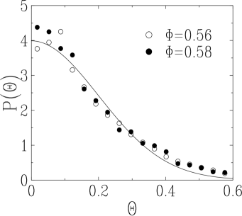
Figure 5: Plot of the normalised distribution of the mean angle $\Theta$ (in radians) of linear bridges of size $n=4$, for both volume fractions. The $\sin\Theta$ Jacobian has been duly divided out, explaining thus the larger statistical errors at small angles. Full lines: common fit to (half) a Gaussian law.

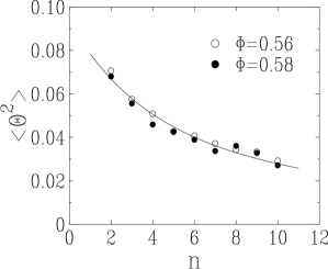
Figure 6: Plot of the variance of the mean angle of a linear bridge, against size $n$, for both volume fractions. Full line: common fit to the first (stationary) term of (2.10), yielding $\sigma_{\rm eq}^{2}=0.093$ and $a=0.55$. The ‘transient’ effects of the second term of (2.10) are invisible with the present accuracy.

2.4 Discussion

We end this section with the following remarks. First, more subtle effects, including the effects of transients via the second term of (2.10), and the dependence of the parameters $\sigma_{\rm eq}^{2}$ and $a$ on the packing fraction $\Phi$, are deserving of further investigation. Second, we might expect that with increasing density $\Phi$, branched structures would become more and more common; linear bridge formation, with its ’sequential’ progressive attachment of independent blobs would then become more and more rare. Our theory should therefore cease to hold at a limit packing fraction $\Phi_{\rm lim}$, which is qualitatively reminiscent of the single-particle relaxation threshold density [8] (see section $3$). Finally, our investigations suggest that long-lived bridges are natural indicators of sustained inhomogeneities in granular systems.

3 On angles of repose: bistability and collapse

Typically, the faces of a sandpile are inclined at a finite angle to the horizontal. This is the so-called ’angle of repose’ $\theta_{\rm R}$: in practice, it can take a range of values before spontaneous flow occurs, i.e., the sandpile becomes unstable to further deposition. The limiting value of this pre-avalanching angle is known as the maximal angle of stability $\theta_{\rm m}$ [6]. Also, as a result of their athermal nature, sandpiles are strongly hysteretic; this results in bistability at the angle of repose  [23, 24], such that a sandpile can either be stable. or in motion, at any angle $\theta$ such that $\theta_{\rm R}<\theta<\theta_{\rm m}$. Notwithstanding the above, it is possible for a sandpile to undergo spontaneous collapse to the horizontal; this is, in general, a rare event. We propose a theoretical explanation [7] below for both bistability at, and collapse through, the angle of repose via the coupling of fast and slow relaxational modes in a sandpile [1].

3.1 Coupled nonlinear equations: dilatancy vs. the angle of repose

Our basic picture is that fluctuations of local density are the collective excitations responsible for stabilising the angle of repose, and for giving it its characteristic width,

$$\delta\theta_{\rm B}=\theta_{\rm m}-\theta_{\rm R},$$ (3.1)

known as the Bagnold angle [22]. Such density fluctuations may arise from, for instance, shape effects [9] or friction [6, 25]; they are the manifestation in our model of Reynolds dilatancy [26].

The dynamics of the angle of repose $\theta(t)$ and of the density fluctuations $\phi(t)$ are described [7] by the following stochastic equations, which couple their time derivatives $\dot{\theta}$ and $\dot{\phi}$:

$$\dot{\theta}=-a\theta+b\phi^{2}+\Delta_{1}\,\eta_{1}(t),$$ (3.2)

$$\dot{\phi}=-c\phi+\Delta_{2}\,\eta_{2}(t).$$ (3.3)

The parameters $a$, …, $\Delta_{2}$ are phenomenological constants, while $\eta_{1}(t)$, $\eta_{2}(t)$ are two independent white noises such that

$$\langle\eta_{i}(t)\eta_{j}(t^{\prime})\rangle=2\,\delta_{ij}\,\delta(t-t^{\prime}).$$ (3.4)

The first terms in (3.2) and (3.3) suggest that neither the angle of repose nor the dilatancy is allowed to be arbitrarily large for a stable system. The second term in (3.2) affirms that dilatancy underlies the phenomenon of the angle of repose; in the absence of noise, density fluctuations constitute this angle. The term proportional to $\phi^{2}$ is written on symmetry grounds, since the the magnitude (rather than the sign) of density fluctuations should determine the width of the angle of repose. The noise in (3.2) represents external vibration, while that in (3.3) embodies Edwards’ compactivity [14], being related to purely density-driven effects. We note that these equations bear more than a passing resemblance to those in the previous section on orientational statistics of bridges: the underlying reason for this similarity is the idea [5, 7] that bridges form by initially aligning themselves at the angle of repose in a sandpile.

Examining the above equations, we quickly distinguish two regimes. When the material is weakly dilatant ($c\gg a$), so that density fluctuations decay quickly to zero (and hence can be neglected), the angle of repose $\theta(t)$ relaxes exponentially fast to an equilibrium state, whose variance

$$\theta_{\rm eq}^{2}=\displaystyle{\displaystyle\Delta_{1}^{2}\over\displaystyle a}$$ (3.5)

is just the zero-dilatancy variance of $\theta$. The opposite limit, where $c\ll a$, and density fluctuations are long-lived, will be our regime of interest here. When, additionally, $\Delta_{1}$ is small, the angle of repose has a slow dynamics reflective of the slowly evolving density fluctuations. These conditions can be written more precisely as

$$\gamma\ll 1,\qquad\varepsilon\ll 1,$$ (3.6)

in terms of two dimensionless parameters (see (3.13):

$$\gamma=\displaystyle{\displaystyle c\over\displaystyle a},\qquad\varepsilon=\displaystyle{\displaystyle ac^{2}\Delta_{1}^{2}\over\displaystyle b^{2}\Delta_{2}^{4}}=\displaystyle{\displaystyle\theta_{\rm eq}^{2}\over\displaystyle\theta_{\rm R}^{2}}.$$ (3.7)

The parameter $\gamma$, which sets the separation of the fast and slow timescales, is an inverse measure of dilatancy in the granular medium; small values of this imply a granular medium that is ’stiff’ to deformation, resulting from the persistence of density fluctuations. The parameter $\varepsilon$ measures the ratio of fluctuations about the (zero-dilatancy) angle of repose to its full value in the presence of density fluctuations: from this we can already infer that it is a measure of the ratio of the external vibrations to density-driven effects, which are explicitly contained in the ratio ($\displaystyle{\displaystyle\Delta_{1}^{2}\over\displaystyle\Delta_{2}^{4}}$). Realising that external vibrations and density/compactivity respectively drive fast and slow dynamical processes in a granular system, we see that a quantity which measures their ratio has all the characteristics of an effective temperature [1] in the slow dynamical regime of interest to us here. This temperature-like aspect will become much more vivid subsequently, when we discuss the issue of sandpile collapse.

To recapitulate: the regime (3.6) that we will discuss below is characterised as low-temperature and strongly dilatant, governed as it is by the slow dynamics of density fluctuations.

3.2 Bistability within $\delta\theta_{\rm B}$ : how dilatancy ’fattens’ the angle of repose

Suppose that a sandpile is created in regime (3.6) with very large initial values for the angle $\theta_{0}$ and dilatancy $\phi_{0}$. In the initial transient stages, the noises have negligible effect and the decay is governed by the deterministic parts of (3.2) and (3.3):

$$\theta(t)=(\theta_{0}-\theta_{\rm m}){\rm e}^{-at}+\theta_{\rm m}\,{\rm e}^{-2ct},$$ (3.8)

$$\phi(t)=\phi_{0}\,{\rm e}^{-ct},$$ (3.9)

with

$$\theta_{\rm m}\approx\displaystyle{\displaystyle b\,\phi_{0}^{2}\over\displaystyle a}.$$ (3.10)

Thus, density fluctuations $\phi(t)$ relax exponentially, while the trajectory $\theta(t)$ has two separate modes of relaxation. First, there is a fast (inertial) decay in $\theta(t)\approx\theta_{0}\,{\rm e}^{-at}$, until $\theta(t)$ is of the order of $\theta_{\rm m}$; this is followed by a slow (collective) decay in $\theta(t)\approx\theta_{\rm m}\,{\rm e}^{-2ct}$. When $\phi(t)$ and $\theta(t)$ are small enough [i.e., $\phi(t)\sim\phi_{\rm eq}$ and $\theta(t)\sim\theta_{\rm R}$, cf. (3.11) and (3.13)] for the noises to have an appreciable effect, the above analysis is no longer valid. The system then reaches the equilibrium state of the full non-linear stochastic process represented by (3.2) and (3.3), a full analytical solution of which is presented in [7].

In order to get a feeling for the more qualitative features of the equilibrium state, we note first that the equilibrium variance of $\phi(t)$ is:

$$\phi_{\rm eq}^{2}=\displaystyle{\displaystyle\Delta_{2}^{2}\over\displaystyle c}.$$ (3.11)

We see next that to a good approximation, the angle $\theta$ adapts instantaneously to the dynamics of $\phi(t)$ in regime (3.6):

$$\theta(t)\approx\displaystyle{\displaystyle b\,\phi(t)^{2}\over\displaystyle a}.$$ (3.12)

The two above statements together imply that the distribution of the angle $\theta(t)$ is approximately that of the square of a Gaussian variable. The typically observed angle of repose $\theta_{\rm R}$ is the time-averaged value

$$\theta_{\rm R}=\langle\theta\rangle_{\rm eq}=\displaystyle{\displaystyle b\,\phi_{\rm eq}^{2}\over\displaystyle a}=\displaystyle{\displaystyle b\Delta_{2}^{2}\over\displaystyle ac}.$$ (3.13)

Equation (3.12) then reads

$$\theta(t)\approx\theta_{\rm R}\,\displaystyle{\displaystyle\phi(t)^{2}\over\displaystyle\phi_{\rm eq}^{2}}.$$ (3.14)

Equation (3.14) entirely explains the physics behind the multivalued and history-dependent nature of the angle of repose [27, 28]. Its instantaneous value depends directly on the instantaneous value of the dilatancy; its maximal (stable) value $\theta_{\rm m}$ is noise-independent [cf. (3.10)] and depends only on the maximal value of dilatancy that a given material can sustain stably [6]. Sandpiles constructed above this will first decay quickly to it; they will then decay more slowly to a ‘typical’ angle of repose $\theta_{\rm R}$. The ratio of these angles is given by

$${\displaystyle\theta_{\rm m}\over\displaystyle\theta_{\rm R}}=\displaystyle{\displaystyle\phi_{0}^{2}\over\displaystyle\phi_{\rm eq}^{2}},$$ (3.15)

so that $\theta_{\rm m}\gg\theta_{\rm R}$ for $\phi_{0}\gg\phi_{\rm eq}$. Within the Bagnold angle $\delta\theta_{\rm B}$, (i.e. for sandpile inclinations which lie in the range $\theta_{\rm R}<\theta<\theta_{\rm m}$), our simple theory also demonstrates the presence of bistability. Thus, sandpiles submitted to low noise are stable in this range of angles (at least for long times $\sim 1/c$); on the other hand, sandpiles submitted to high noise (such that the effects of dilatancy become negligible in (3.2)) continue to decay rapidly in this range of angles, becoming nearly horizontal at short times $\sim 1/a$.

Our conclusions are that bistability at the angle of repose is a natural consequence of applied noise (tilt [23] or vibration) in granular systems. For sandpile inclinations $\theta$ within the range $\delta\theta_{\rm B}$, sandpile history is all-important: depending on this, a sandpile can either be at rest or in motion at the same angle of repose.

3.3 When sandpiles collapse: rare events, activated processes and the topology of rough landscapes

When sandpiles are subjected to low noise for a sufficiently long time, they can collapse [1], such that the angle $\theta(t)$ vanishes. Such an event is expected to be very rare in the regime (3.6); in fact it occurs only if the noise $\eta_{1}(t)$ in (3.2) is sufficiently negative for sufficiently long to compensate for the strictly positive term $b\phi^{2}$. It can be shown [7] that the equilibrium probability for $\theta$ to be negative, $\Pi={\rm Prob}(\theta<0)$, scales throughout regime (3.6) as:

$$\Pi\approx\displaystyle{\displaystyle(2\varepsilon)^{1/4}\over\displaystyle\Gamma(1/4)}\,{\cal F}(\zeta),\qquad\zeta=\displaystyle{\displaystyle\gamma\over\displaystyle\varepsilon^{1/2}}=\displaystyle{\displaystyle b\Delta_{2}^{2}\over\displaystyle a^{3/2}\Delta_{1}}$$ (3.16)

The scaling function ${\cal F}(\zeta)$ decays [7] monotonically from ${\cal F}(0)=1$ to ${\cal F}(\infty)=0$; to find out when the angle of repose first crosses zero, we should explore the latter limit, i.e. the regime $\zeta\gg 1$. Here, the equilibrium probability of collapse vanishes exponentially fast:

$$\Pi\sim\exp\left(-\displaystyle{\displaystyle 3\over\displaystyle 2}\left(\displaystyle{\displaystyle\gamma^{2}\over\displaystyle\varepsilon}\right)^{1/3}\right).$$ (3.17)

The above suggests that sandpile collapse is an activated process, with a competition between ’temperature’ $\varepsilon$ and ’barrier height’ $\gamma^{2}$. Collapse events occur at Poissonian times, with an exponentially large characteristic time given by an Arrhenius law:

$$\tau\sim 1/\Pi\sim\exp\left(\displaystyle{\displaystyle 3\over\displaystyle 2}\left(\displaystyle{\displaystyle\gamma^{2}\over\displaystyle\varepsilon}\right)^{1/3}\right).$$ (3.18)

The stretched exponential with a fractional power of the usual ’barrier-height-to-temperature ratio’ $\gamma^{2}/\varepsilon$ is suggestive of glassy dynamics [3]; it also reinforces the idea that sandpile collapse is a rare event.

While the reader is referred to a longer paper [7] for the derivation of the stretched exponential, the physics behind it is readily understood by means of an exact analogy with the problem of random trapping [29], which we outline below.

Consider a Brownian particle in one dimension, diffusing (with diffusion constant $D$) among a concentration $c$ of Poissonian traps. Once a trap is reached, the particle ceases to exist, so that its survival probability $S(t)$ is also the probability that it has not encountered a trap until time $t$. Assuming a uniform distribution of starting points, the fall-off of this probability can be estimated by first computing the probability of finding a large region of length $L$ without traps, and then weighting this with the probability that a Brownian particle survives within it for a long time $t$:

$$S(t)\sim\int_{0}^{\infty}\exp\left(-cL-\displaystyle{\displaystyle\pi^{2}Dt\over\displaystyle L^{2}}\right)\,{\rm d}L.$$ (3.19)

The first exponential factor $\exp(-cL)$ is the probability that a region of length $L$ is free of traps, whereas the second exponential factor is the asymptotic survival probability of a Brownian particle in such a region, $\exp(-Dq^{2}t)$. The integral is dominated by a saddle-point at $L\approx\left(\displaystyle{\displaystyle 2\pi^{2}Dt\over\displaystyle c}\right)^{1/3}$, whence we recover the well-known estimate

$$S(t)\sim\exp\left(-\displaystyle{\displaystyle 3\over\displaystyle 2}\left(2\pi^{2}c^{2}Dt\right)^{1/3}\right).$$ (3.20)

Notice the similarity in the forms of (3.17) and (3.20); it turns out that the steps in their derivations are identical [7], and form the basis of an exact analogy. In turn the analogy allows us to formulate an optimisation-based approach to sandpile collapse, which makes for a much more intuitive grasp of its physics.

Accordingly, let us visualise the angle $\theta$ as an ’exciton’ whose ’energy levels’ are determined by the magnitude of $\theta$. It diffuses with temperature $\varepsilon$ in a frozen landscape of $\phi$ (dilatancy) barriers of typical energy $\gamma$. Only if it succeeds in finding an unusually low barrier can it escape via  (3.17), to reach its ground state ($\theta=0$) - this of course corresponds to sandpile collapse. Taking the analogy a step further, we visualise the exciton as ’flying’ at a ’height’ $\theta$, surrounded by $\phi$-peaks of typical ’height’ $\gamma$ in a rough landscape. Flying too low would cause the $\theta$ exciton to hit a $\phi$ barrier fast, while flying too high would cause the exciton to miss the odd low barrier. It turns out [7] that flying at $\theta\sim\varepsilon^{1/3}$ allows the exciton to escape via (3.17) (cf. the arguments leading to $L\sim t^{1/3}$ above). Translating back to the scenario of sandpile angles, the above arguments imply the following: angles of repose that are too low are unsustainable for any length of time, given dilatancy effects, while angles that are too large will resist collapse. Thus optimal angles for sandpile collapse are found to scale as $\theta\sim\varepsilon^{1/3}$; sandpiles with these inclinations show a finite, if small, tendency to collapse via (3.17).

Clearly, the frequency of collapse will depend on the topology of the $\phi$-landscape; the form (3.17) was valid for a landscape with Gaussian roughness [7]. What if the landscape is much rougher or smoother than this? - to answer this question, we look at two opposite extremes of non-Gaussianness.

First, let us assume that density fluctuations are peaked around zero; typical barriers are low, and the $\phi$-landscape is much flatter than Gaussian. The exciton’s escape probability ought now to be greatly increased. This is in fact the case [7]; it can be shown that in the $\gamma\to 0$ limit, the collapse probability scales as $\varepsilon^{1/4}$. Switching back to the language of sandpiles, this limit corresponds to a nearly non-dilatant material; it results in a ‘liquid-like’ scenario of frequent collapse, where a finite angle of repose is hard to sustain under any circumstances.

In the opposite limit of an extremely rough energy landscape, where large values of $\phi$ are more frequent than in the Gaussian distribution, one might expect the escape probability of the $\theta$ exciton to be greatly reduced. If, for example, the jaggedness of the landscape is such that $|\phi(t)|$ is always larger than some threshold $\phi_{\rm th}$, the stretched exponential in (3.17) reverts (in the $\varepsilon\ll 1$ regime considered) to an Arrhenius law in its usual form:

$$\Pi\sim\exp\left(-\displaystyle{\displaystyle(\phi_{\rm th}/\phi_{\rm eq})^{4}\over\displaystyle 2\varepsilon}\right).$$ (3.21)

In the language of sandpiles, this limit corresponds to strongly dilatant material; here, as one might expect, sandpile collapse is even more strongly inhibited than in (3.17). Wet sand for example, is strongly dilatant; its angles of repose can be far steeper than usual, and still resist collapse.

3.4 Discussion

The essence of our theory above is that dilatancy is responsible for the existence of the angle of repose in a sandpile. We claim further that bistability at the angle of repose results from the difference between out-of-equilibrium and equilibrated dilatancies. We are also able to provide an analytical confirmation of the following everyday observation: weakly dilatant sandpiles collapse easily, while strongly dilatant ones bounce back.

4 Compaction of disordered grains in the jamming limit: sand on random graphs

Granular compaction is characterised by a competition between fast and slow degrees of freedom [1]; when voids abound, individual grains can quickly move into these to suit their convenience. As the jamming limit is approached, clusters of grains need to rearrange in order better to fill remaining partial voids: this process is necessarily slow, and eventually leads to dynamical arrest [3].

The modelling of granular compaction has been the subject of considerable effort. Early simulations of shaken hard sphere packings [10], carried out in close symbiosis with experiment [30], were followed by lattice-based theoretical models [31, 32]; the latter could not, of course, incorporate the reality of a disordered substrate. Mean-field models [33] which could incorporate such disorder could not, on the other hand, impose the finite connectivity of grains included in Refs. [10, 31, 32]. It was to answer the need of an analytically tractable model which incorporated finitely connected grains on fully disordered substrates, that we introduced [8] random graph models of granular compaction.

Why random graphs? First, random graphs [34] are the simplest structures with a finite number of neighbours. Finite connectivity is a key property of grains in a sandpile with a gamut of consequences, ranging from kinetic constraints [35] to cascade processes in granular compaction [8]. Second, random graphs are among the simplest fully disordered constructs where, despite the existence of defined neighbourhoods of a site, no global symmetries exist. Disorder is an equally key feature of granular matter, even at the highest densities; its consequences include the presence of a range of coordination numbers [10] for any sandpile, corresponding to locally varying neighbourhoods of individual grains, a feature which can be incorporated via locally fluctuating connectivities [8] in random graphs.

Having motivated our choice of random graphs as a basis, we proceed below to describe our spin model of granular compaction.

4.1 The three-spin model: frustration, metastability and slow dynamics

The guiding factor in our choice of spin model is that it be the simplest model with frustration, metastability and slow dynamics; we will discuss the last two later, but remark at the outset that geometrical frustration is crucial to any study of granular matter. This concerns the fruitless competition between grains which try - and fail - to fill voids in the jamming limit, due either to geometric constraints on their mobility, or because of incompatibilities in shape or size. Our way of modelling this is via multi-spin interactions on plaquettes on a random graph [8]. We choose in particular a 3-spin Hamiltonian on a random graph (see Fig. 7) where $N$ binary spins $S_{i}=\pm 1$ interact in triplets:

$$H=-\rho N=-\sum_{i<j<k}C_{ijk}S_{i}S_{j}S_{k}$$ (4.1)

Here, the variable $C_{ijk}=1$ with $i<j<k$ denotes the presence of a plaquette connecting sites $i,j,k$, while $C_{ijk}=0$ denotes its absence. Choosing $C_{ijk}=1(0)$ randomly with probability $2c/N^{2}$ ($1-2c/N^{2}$) results in a random graph, where the number of plaquettes connected to a site is distributed with a Poisson distribution of average $c$ - this exemplifies the locally varying connectivities mentioned above. The connection with granular compaction is made in accordance with Edwards’ hypothesis [14]: we interpret the local contribution to the energy in different configurations of the spins as the volume occupied by grains in different local orientations.

Figure 7: A part of a random graph with triplets of sites forming plaquettes illustratng its local treelike structure (no planarity or geometric sense of distance are implied).

This Hamiltonian has been studied on a random graph in various contexts [36, 37]. It has a trivial ground state where all spins point up and all plaquettes are in the configuration $+++$ giving a contribution of $-1$ to the energy. Yet, locally, plaquettes of the type $--+,-+-,+--$ (satisfied plaquettes) also give the same contribution, although one may not be able to cover the entire graph with these four types of plaquettes in equal proportions. This degeneracy of the four configurations of plaquettes with $s_{i}s_{j}s_{k}=1$ results in frustration, via the competition between satisfying plaquettes locally and globally. In the former case, all states with even parity may be used, resulting in a large entropy and in the latter, only the $+++$ state may be used. Such frustration eventually leads to slow dynamics.

This mechanism has a suggestive analogy in the concept of geometrical frustration of granular matter, if we think of plaquettes as granular clusters. When grains are shaken, they rearrange locally, but locally dense configurations can be mutually incompatible. Voids could appear between densely packed clusters due to mutually incompatible grain orientations between neighbouring clusters. The process of compaction in granular media consists of a competition between the compaction of local clusters and the minimisation of voids globally .

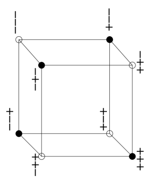
Figure 8: The phase space of three spins connected by a single plaquette. Configurations of energy $-1$ (the plaquette is satisfied) are indicated by a black dot, those of energy $+1$ (the plaquette is unsatisfied) are indicated by a white dot

Another key feature of this model is the existence of metastable states. We note from Figure 8 that two spin flips are required to take a given plaquette from one satisfied configuration to another; an energy barrier thus has to be crossed in any intermediate step between two satisfied configurations. This has a mirror image in the context of granular dynamics, where compaction follows a temporary dilation; for example, a grain could form an unstable (’loose’) bridge with other grains before it collapses into an available void beneath the latter [5, 10]. This mechanism, by which an energy barrier has to be crossed in going from one metastable state to another, is an important ingredient in models of granular compaction [38].

4.2 How we tap the spins - dilation and quench phases

Our tapping algorithm is a simplified version of the tapping dynamics used in cooperative Monte Carlo simulations of sphere shaking [10]. We treat each tap as consisting of two phases. First, during the dilation phase, grains are provided with free volume to move into; next, in the quench phase, they are allowed to relax until a mechanically stable configuration is reached.

More technically, the dilation phase is modelled by a single sequential Monte Carlo sweep of the system at a dimensionless temperature $\Gamma$. A site $i$ is chosen at random and flipped with probability $1$ if its spin $s_{i}$ is antiparallel to its local field $h_{i}$, with probability $\exp(-h_{i}/\Gamma)$ if it is not, and with probability $0.5$ if $h_{i}=0$. This procedure is repeated $N$ times. Sites with a large absolute value of the local field $h_{i}$ thus have a low probability of flipping into the direction against the field; such spins may be thought of as being highly constrained by their neighbours. The dynamics of our ’thermal’ dilation phase differs from the ’zero-temperature’ dynamics used in [40] where a certain fraction of spins is flipped regardless of the value of their local field. Our choice [8] reflects the following physics: if grains are densely packed (’strongly bonded’ to their neighbours), they are unlikely to be displaced during the dilation phase of vibration.

The grains are then allowed to relax via a $\Gamma=0$ quench, which lasts until the system has reached a blocked configuration [41], where each site $i$ has $s_{i}=\mbox{sgn}(h_{i})$ or $h_{i}=0$: thus, each grain is either aligned with its local field, or it is a ’rattler’ [42]. Thus, at the end of each tap (dilation $+$ quench), the system will be in a physically stable configuration [10].

4.3 The compaction curve

Among the most important of our results is the compaction curve obtained by tapping our model granular medium for long times. This is shown in Figure 9, where three regimes of the dynamics can be identified. In the first regime, fast individual dynamics predominates, while in the second, one sees a logarithmic growth of the density via slow collective dynamics.The last regime consists of system-spanning density fluctuations in the jamming limit, where our quantitative agreement with experiment [43] allows us to propose a cascade theory of compaction during jamming.

Figure 9: Compaction curve at connectivity $c=3$ for a system of $10^{4}$ spins (one spin is flipped at random per tap). The data stem from a single run with random initial conditions and the fit (dashed line) follows (4.2) with parameters $\rho_{\infty}=.971$, $\rho_{0}=.840$, $D=2.76$, and $\tau=1510$. The long-dashed line (top) indicates the approximate density $0.954$ at which the dynamical transition occurs, the long-dashed line (bottom) indicates the approximate density $0.835$ at which the fast dynamics stops, the single-particle relaxation threshold.

4.3.1 Fast dynamics till SPRT: each grain for itself!

At the end of the first tap, each grain is connected to more unfrustrated than frustrated clusters. This is a direct result of the first tap being a zero-temperature quench: any site where this was not the case would simply flip its spin. More generally, a fast dynamics occurs in this regime whereby single grains locally adopt the orientation that, finally, optimises their density; this density $\rho_{0}$ has been termed [8] the single-particle relaxation threshold (SPRT).

If we neglect correlations between the local fields of neighbouring sites, we can arrive at a simple population dynamics model of the fast dynamics, details of which can be found in [8]. It yields a value of the SPRT, $\rho_{0}=0.835$ (shown as a dotted line in Figure 9) which is much higher than the value of the density $\rho(=0.49)$ of a typical blocked configuration.

This is quite an extraordinary result; it implies that despite the exponential dominance of blocked configurations, random initial conditions preferentially select a higher density corresponding to the SPRT $\rho_{0}$. This prediction of an overshoot in the density achieved by fast dynamics has also, strikingly, been confirmed in independent lattice-based models [31] of granular compaction, and points to a strong non-ergodicity in the fast dynamics of individual grains. We will discuss this further in Section $5.3$.

Another significant feature of this regime is that a fraction of spins is left with local fields exactly equal to zero, which thus keep changing orientation [44]. These are manifestations in our model of ’rattlers’ [42], i.e. grains which keep changing their orientation within well-defined clusters [10]. They will later (cf. Section $5.3$) be used as a tool to probe the statistics of blocked configurations [8].

To summarize: each grain reaches its locally optimal configuration via fast individual dynamics, resulting in the attainment of the SPRT density. All dynamics after this point is perforce collective.

4.3.2 Slow dynamics of granular clusters: logarithmic compaction.

The second stage of our tapping dynamics is fully collective: it removes some of the remaining frustrated plaquettes as clusters slowly rearrange themselves. A logarithmically slow compaction results [30, 31], leading from the SPRT density $\rho_{0}$ to the asymptotic density $\rho_{\infty}$. The resulting compaction curve may be fitted, with $D$ and $\tau$ being characteristic constants, to the well-known logarithmic law [30]:

$$\rho(t)=\rho_{\infty}-(\rho_{\infty}-\rho_{0})/(1+1/D\,\ln(1+t/\tau))\ ,$$ (4.2)

This can be written more transparently as $1+t(\rho)/\tau=\exp{\{D\displaystyle{\displaystyle\rho-\rho_{0}\over\displaystyle\rho_{\infty}-\rho}\}}\$, a form which makes clear that the dynamics becomes slow (logarithmic) as soon as the density reaches $\rho_{0}$. Although most grains are firmly held in place by their neighbours in this regime, cascade-like changes of orientation can occur. For example, if some grains change orientation during the dilation phase, this would change the constraints on their neighbours; importantly, the freer dynamics of rattlers could also alter local fields in their neighbourhood, and cause previously blocked grains to reorient. Reorientation in cascades [8] would then ensue, leading to collective granular compaction upto the asymptotic density $\rho_{\infty}$. We identify this with the density of random close packing [45] (RCP) and associate it with a dynamical phase transition [46, 47].

4.3.3 Cascades at the dynamical transition.

With increasing density, free-energy barriers rise up causing the dynamics to slow down according to (4.2). The point where the height of these barriers scales with the system size marks a breaking of the ergodicity of the dynamics; an exponential number of valleys appears in the free-energy landscape. Our theoretical [8] value for the dynamical transition, shown as a horizontal line in Figure 9, is in good agreement with the asymptotic density $\rho_{\infty}$ reached (numerically) by the tapping dynamics.

Also shown in Figure 9 are marked fluctuations around the logarithmic compaction law, especially as the jamming limit is approached; their correlations over several octaves have been the subject of detailed experimental investigations [43]. To compare the results of our model with experiment, we follow [43] and use Fourier transforms to plot the power spectrum of the timeseries $\rho(t)$ (in different frequency bands) against time in Figure 10.

Figure 10: The density fluctuations as a function of time resulting from 1024 taps are plotted as the topmost trace. The successive plots are of the power spectrum against time, in different frequency octaves. The power in the first octave (frequency 1/(1024 taps) -2/(1024 taps)) is the bottommost trace, second octave (frequency 2/(1024 taps) - 4/(1024 taps)), above it, and so on to the top. Note that the fluctuations of the power in the different frequency bands are strongly correlated; they correspond to sudden changes in the density (topmost trace).

Our results indicate, as in the experimental data, that there are ’bursts’ in the power spectrum fluctuations: our decomposition of these bursts over several octaves shows that they are caused by strong correlations of noise power over a wide range of frequencies. Importantly, the correlation matrices we obtain [8] are in quantitative agreement with experiment [43].

In our model, we can trace such bursts as being due to cascades of spin-flips. As mentioned before, these arise from the change in local fields caused by the flipping of a single spin (or several spins); this instability propagates through ever larger neighbourhoods, causing correlated bursts in noise power fluctuations. Note that this cascade mechanism is entirely absent from generic fully connected models [33], where each spin interacts with all spins in the system. Interestingly, it is also absent from the finitely-connected parking-lot model [48]; this is because the creation and filling of ’parking lots’ by ’cars’ in that model does not cause the appearance of further parking lots, in the way spins flips may trigger a cascade. Put another way, the absence of competition between individual and collective interactions in the parking-lot [48] model results in an absence of cascades there, despite its finite connectivity.

We use the above insights to argue [8] that in real granular media, the observed correlations [43] of density fluctuations are due to a cascade process in granular compaction near the jamming limit. Here, orientational/positional changes in strongly constrained grains give rise to propagating instabilities, leading to a near-global rearrangement of the granular medium. Pictorially, the movement of a single grain in this regime is only possible as the consequence of a system-wide cooperative motion of grains: this leads to sharp changes in overall density, and to the observed ’bursts’ in the power spectrum of density fluctuations [43].

4.4 Realistic amplitude cycling; how granular media jam at densities lower than close-packed.

Our random graphs model has also been used to simulate amplitude cycling, an experimental [30] protocol on tapped granular media. Here, the granular medium is tapped at a given amplitude $\Gamma$ for a time $\tau$, after which its amplitude is changed by an infinitesimal $\delta\Gamma$; this process is repeated for cycles of increasing and decreasing $\Gamma$. The control parameter turns out to be the so called ’ramp rate’, which is the ratio $\delta\Gamma/\tau$; this is a measure [31] of the ’equilibration’ allowed to the granular medium. Clearly low values of this will correspond to quasi-static processes, while large values will correspond to near-adiabaticity.

The most simple-minded application of this protocol in our model results in the scenario of Figure 11. At both high and low cycling rates, the density $\rho$ first reaches the SPRT $\rho_{0}$, increases with increasing amplitude, and decreases again at large values of $\Gamma$. Thereafter, $\rho$ always decreases with increasing $\Gamma$. The part of the curve where $\Gamma$ is increased for the first time has been termed [30] the irreversible branch; the reversible branch refers to the trajectory traced out by all successive increases and decreases of tapping amplitude. The results of Figure 11, in agreement with many other models [31, 38, 49], suggest that as the ramp rate is decreased, the system will eventually attain the RCP density $\rho_{\infty}$. In particular, these models predict that in the limit of near-zero ramp rates, the irreversible branch disappears, with $\rho$ becoming a single-valued function of $\Gamma$.

Figure 11: Amplitude cycling: $\Gamma$ is varied in both directions between $0$ to $2$ at two rates $\delta\Gamma=10^{-4},10^{-5}$ per tap. with $\tau=1$. The lower ramp rate (shown by the dotted line) results in a higher final density.

This prediction is in direct contradiction to the experimental results of [30]; these suggest that at least for experimentally realisable times, low-amplitude shaking does not result in RCP being reached. Instead, they suggest that some grains in the jamming limit of a granular assembly are so strongly constrained that they will never be displaced by low-amplitude taps.

In order to model the above experimental scenario, we modify the simplest picture of amplitude cycling presented above. First, we realise that in the dynamics of our model described thus far, sites with a high local field (corresponding to strongly constrained grains) may be flipped at any finite value of $\Gamma$ with a correspondingly small but finite probability. This is what eventually leads the system to the RCP density $\rho_{\infty}$.

To prevent this drift to RCP, one could naively think of introducing a threshold in local fields such that spins with fields above this threshold are not flipped. It turns out [8], however, that this is insufficient; the orientational dynamics of neighbouring spins will always loosen the constraints on previously blocked spins in the end, and lower their local fields below any given threshold. The above implies that the constraints on grains are not related to orientational frustration alone; it was suggested [8] that they might also be mechanical in nature, related to force networks [17] between grains. Further, it seemed reasonable to suppose that such effectively immobile [51] ’blockages’ could only be removed kinetically by the imposition of large intensity ($\Gamma$) vibrations.

Accordingly, the concept of low-amplitude pinning of grains was introduced [8]: assign to each site $i$ a real number $r_{i}$ between zero and one, such that only grains with $r_{i}<\Gamma$ (mechanically constraining forces less than external vibration intensity) will be free to move. This modification could in principle lead to a lower value of $\rho_{\infty}$ after amplitude recycling: for example, spin plaquettes (granular clusters) generated during the high-amplitude part of the cycle, would be effectively immobile at lower amplitudes, leading to wasted space.

However, this too is insufficient to stop the evolution of the system to $\rho_{\infty}$. It turns out [8] that jamming at lower densities can only be achieved if low-amplitude pinning is combined with the choice of an extremely low ramp rate, via a large ’equilibration time’ $\tau$. If this is done, grains are allowed to ’equilibrate’ at each amplitude, thus making sure that a steady-state of the density is always reached. This leads, finally, to the low-amplitude immobilisation of granular clusters created at high amplitudes, to the consequent blocking of voids, and hence to ’jamming’  [30, 50] at densities lower than RCP (see Figure 12)

Figure 12: The asymptotic density for tapping amplitudes ranging from $\Gamma=0.2$ to $\Gamma=2$ in steps of $0.2$. The density measured after $10^{7}$ taps at each amplitude and convergence to a steady-state each time was checked.

Our results [8] on modified amplitude cycling thus indicate that it is important to have mechanical pinning as well as long equilibration times [52] for jamming to occur. In fact, the random configurations of immobile spins at each value of $\Gamma$ can be viewed [8] as an additional quenched disorder, and their effect on neighbouring mobile spins, as an additional random local field. Our results demonstrate also a rather fundamental difference between excitations in glassy systems and granular media. In glasses, one would expect the configurations of spins reached at high values of temperature and subsequently frozen, immediately to alter the behaviour of the system at lower values of temperature. In athermal media like granular systems, however, it is important to allow equilibration at each value of the shaking intensity $\Gamma$, in order even to begin to observe the hysteretic effects which result in jamming at lower-than-RCP densities.

4.5 Discussion

In the above, we have presented a finitely connected spin model on random graphs [8], with the aim of examining the compaction of tapped granular media. Fast non-ergodic relaxation of individual grains terminated at the SPRT density, in our compaction curve; collective relaxation followed, manifest first by logarithmic compaction, and next by system-wide density fluctuations around RCP, both of which match experimental results [30, 43]. Our model explains the latter in terms of a cascade process that occurs near the jamming limit of granular matter. Also, in contradistinction to other models [31, 38, 49], our results indicate that jamming at densities lower than RCP occurs as a result of competition between mechanical and orientational frustration, during amplitude cycling. We leave the discussion of the configurational entropies [8, 53] generated by our tapping algorithm to the concluding section of this article.

5 Shape matters

In the concluding section of this review, we explore the effect of grain shapes in granular compaction. Our model is based on the following picture. Consider a box of sand in the presence of gravity; for ease of visualisation, we think of this as being constituted of vertical columns. In the jamming limit, diffusion of grains between columns is inhibited [31] due to the absence of holes (grain-sized voids); compaction proceeds instead by grain reorientation within each column [9] to minimise the size of the partial voids that persist. This intuitive picture is verified by results of computer simulations [10] which show that correlations in the transverse (inter-column) direction are negligible compared to those in the longitudinal (intra-column) direction. We thus focus on a column model of grains in the jamming limit [9].

Each ordered grain occupies one unit of space, while each disordered grain occupies $1+\varepsilon$ units of space, with $\varepsilon$ a measure of the partial void trapped by misorientation. A reorientation of the grain to an ordered (‘space-saving’) state frees up the partial void, for use by other grains to reorient themselves. This cascade-like picture of compaction in the jamming limit resembles that presented in the previous section, where random graph models [8] were discussed. Also, as there, the response of grains to external dynamics is via the local minimisation of void space modelled by a local field.

5.1 A model of regular and irregular grains

In our column model, grains are indexed by their depth $n$ measured from the free surface. Each grain can be in one of two orientational states – ordered ($+$) or disordered ($-$) – the ‘spin’ variables $\{\sigma_{n}=\pm 1\}$ thus uniquely defining a configuration. Exactly as in the random graphs model [8] presented above, a local field $h_{n}$ constrains the temporal evolution of spin $\sigma_{n}$, such that excess void space is minimised.

In the presence of a vibration intensity $\Gamma$, grains reorient with an ease that depends on their depth $n$ within the column (grains at the free surface must clearly be the freest to move!), as well as on the local void space $h_{n}$ available to them. The transition probabilities governing this are:

$$w\bigl{(}\sigma_{n}=\pm\to\sigma_{n}=\mp\bigr{)}=\exp\bigl{(}-n/\xi_{\rm dyn}\mp h_{n}/\Gamma\bigr{)}.$$ (5.1)

The dynamical length $\xi_{\rm dyn}$ [9, 31] effectively defines the boundary layer of the column; within this dynamics are fast, while well beyond it, they are slow. The local field $h_{n}$ is a measure of excess void space [6]:

$$h_{n}=\varepsilon\,m^{-}_{n}-m^{+}_{n},$$ (5.2)

where $m^{+}_{n}$ and $m^{-}_{n}$ are respectively the numbers of $+$ and $-$ grains above grain $n$. The definition Equation (5.2) is such that a transition from an ordered to a disordered state for grain $n$ is hindered by the number of voids that are already above it, as might be expected for an ordering field in the jamming limit.

In the $\Gamma\to 0$ limit of zero-temperature dynamics [8], the probabilistic rules (5.1) become deterministic: the expression $\sigma_{n}=\mathop{\rm sign}\nolimits\,h_{n}$ (provided $h_{n}\neq 0$) determines the ground states of the system. Frustration [2] manifests itself for $\varepsilon>0$, which leads to a rich ground-state structure, whose precise nature depends on whether $\varepsilon$ is rational or irrational. We mention for completeness that the case $\varepsilon<0$ discussed in earlier work [31] corresponds to a complete absence of frustration and a single ground state of ordered grains.

For irrational $\varepsilon$, no local field $h_{n}$ can ever be zero (cf. (5.2)). Noting that irrational values of $\varepsilon$ denote shape irregularity, we conclude that the excess void space is nonzero even in the ground state of jagged grains. Their ground state, far from being perfectly packed, turns out [9] to be quasiperiodic.

Regularly shaped grains correspond to rational $\varepsilon=p/q$, with $p$ and $q$ mutual primes. We see from (5.2) that now, some of the $h_{n}$ can vanish; these correspond, as noted in the previous section, to rattlers. A rattler at depth $n$ thus has a perfectly packed column above it, so that it is free to choose its orientation [8, 9, 42]. For regular grains in their ground state, rattlers occur periodically (as in crystalline packings!) at points such that $n$ is a multiple of the period $p+q$.. Every ground state is thus a random sequence of two patterns of length $p+q$, each containing $p$ ordered and $q$ disordered grains; this degeneracy leads to a zero-temperature configurational entropy or ground-state entropy $\Sigma=\ln 2/(p+q)$ per grain.

5.2 Zero-temperature dynamics: (ir)retrievability of ground states, density fluctuations and anticorrelations

Regular and irregular grains behave rather differently when submitted to zero-temperature dynamics. The (imperfect) but unique ground state for irregular grains is rapidly retrieved; the perfect (and degenerate) ground states for regular grains never are, resulting in density fluctuations.

We recall the rule for zero-temperature dynamics:

$$\sigma_{n}\to\mathop{\rm sign}\nolimits h_{n}.$$ (5.3)

Starting with irregular grains (with a given irrational value of $\varepsilon$) in an initially disordered state, one quickly recovers the ground state with zero-temperature dynamics. The ground state in fact propagates ballistically from the free surface to a depth $L(t)\approx V(\varepsilon)\,t$ [9] at time $t$, while the rest of the system remains in its disordered initial state. When $L(t)$ becomes comparable with $\xi_{\rm dyn}$, the effects of the free surface begin to be damped. In particular for $t\gg\xi_{\rm dyn}/V(\varepsilon)$ we recover the logarithmic coarsening law $L(t)\approx\xi_{\rm dyn}\ln t$, also seen in other theoretical models [8, 31] of the slow relaxation of tapped granular media [30]. To recapitulate, the ground state for irregular grains is quickly (ballistically) recovered with zero-temperature dynamics, until the boundary layer $\xi_{\rm dyn}$ is reached; below this, the column is essentially frozen, and coarsens only logarithmically.

For regular grains with rational $\varepsilon$, the local field $h_{n}$ in (5.3) vanishes for rattlers. Their dynamics is stochastic even at zero temperature, since they have a choice of orientations: a simple way to update them is according to the rule $\sigma_{n}\to\pm 1$ with probability $1/2$. This stochasticity results in an intriguing dynamics even well within the boundary layer $\xi_{\rm dyn}$, while the dynamics for $n\gg\xi_{\rm dyn}$ is as before logarithmically slow [9].

In what follows, we will focus on the fast dynamics within the boundary layer. Our main result is that zero-temperature dynamics does not drive the system to any of its degenerate ground states, but instead engenders a fast relaxation to a non-trivial steady state, independent of initial conditions, which consists of unbounded density fluctuations. This recalls density fluctuations close to the jamming limit [8, 30], in other studies of granular compaction.

Figure 13: Log-log plot of $W_{n}^{2}=\langle h_{n}^{2}\rangle$ against depth $n$, for zero-temperature dynamics with $\varepsilon=1$. Full line: numerical data. Dashed line: fit to asymptotic behaviour leading to (5.4) (after [9]).

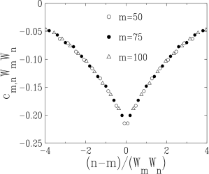
Figure 14: Scaling plot of the orientation correlation function $c_{m,n}$ for $n\neq m$ in the zero-temperature steady state with $\varepsilon=1$, demonstrating the validity of (5.5) and showing a plot of (minus) the scaling function $F$ (after [9]).

Fig. 13 shows the variation of these density fluctuations as a function of depth $n$:

$$W_{n}^{2}=\langle h_{n}^{2}\rangle\approx A\,n^{2/3},\quad A\approx 0.83.$$ (5.4)

The fluctuations are approximately Gaussian, with a definite excess at small values: $|h_{n}|\sim 1\ll W_{n}$. We recall that non-Gaussianness was also observed in experiments on density fluctuations in tapped granular media [43]; in our theory here, we interpret it in terms of grain (anti)correlations. If grain orientations were fully uncorrelated, one would have the simple result $\langle h_{n}^{2}\rangle=n\varepsilon$, while (5.4) implies that $\langle h_{n}^{2}\rangle$ grows much more slowly than $n$.

It turns out that at least within a dynamical cluster of radius $n^{2/3}$) [9], the orientational displacements of each grain are fully anticorrelated. Fig. 14 shows that the orientation correlations $c_{m,n}=\langle\sigma_{m}\sigma_{n}\rangle$ scale as [9]

$$c_{m,n}\approx\delta_{m,n}-\displaystyle{\displaystyle 1\over\displaystyle W_{m}W_{n}}\,F\!\left(\displaystyle{\displaystyle n-m\over\displaystyle W_{m}W_{n}}\right),$$ (5.5)

where the function $F$ is such that $\int_{-\infty}^{+\infty}F(x)\,{\rm d}x=1$. We find also that, within such a dynamical cluster, the fluctuations of the orientational displacements are totally screened: $\sum_{n\neq m}c_{m,n}\approx-c_{m,m}=-1$. These results recall the anticorrelations in grain displacements observed in independent simulations of shaken hard spheres close to jamming [10]; there they corresponded to compaction via bridge collapse, as upper and lower grains in bridges [6] collapsed onto each other, releasing void space.

5.3 Rugged entropic landscapes: Edwards’ or not?

The most remarkable feature of our column model is, arguably, the rugged landscape of microscopic configurations visited during the steady state of zero-temperature dynamics (for regular grains); this is all the more striking because the macroscopic entropy is flat, in agreement with Edwards’ hypothesis [14].

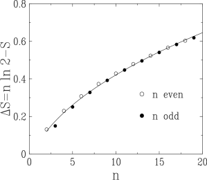
Figure 15: Plot of the measured entropy reduction $\Delta S$ in the zero-temperature steady state with $\varepsilon=1$, against $n\leq 19$. Symbols: numerical data, for $t\sim 10^{9}$ and $n\approx 20$. Full line: fit $\Delta S=(62\ln n+53)10^{-3}\,n^{1/3}$.

The entropy of the steady state of zero-temperature dynamics is defined by the usual Boltzmann formula

$$S=-\sum_{\cal C}p({\cal C})\ln p({\cal C}),$$ (5.6)

where $p({\cal C})$ is the probability that the system is in the orientation configuration ${\cal C}$ in the steady state, and the sum runs over all the $2^{n}$ configurations of a system of $n$ grains. This can be estimated theoretically by using (5.4). Consider $n$ as a fictitious discrete time, with the local field $h_{n}$ as the position of a random walker at time $n$. For a free lattice random walk of $n$ steps, one has $\langle h_{n}^{2}\rangle=n$; as all configurations are equiprobable. the entropy reads $S_{\rm flat}=n\ln 2$. For a column of regularly shaped grains, our model predicts instead $\langle h_{n}^{2}\rangle=W_{n}^{2}\ll n$; the entropy $S$ of our random walker is therefore reduced with respect to $S_{\rm flat}$. The entropy reduction [54] $\Delta S=S_{\rm flat}-S=n\ln 2-S$ can be estimated [9] to be

$$\Delta S\sim\sum_{m=1}^{n}\displaystyle{\displaystyle 1\over\displaystyle W_{m}^{2}}\sim n^{1/3}.$$ (5.7)

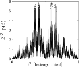
Figure 16: Plot of the normalised probabilities $2^{12}\,p({\cal C})$ of the configurations of a column of 12 grains in the zero-temperature steady state with $\varepsilon=1$, against the configurations ${\cal C}$ in lexicographical order. The empty circles mark the $2^{6}=64$ ground-state configurations, which turn out to be the most probable (after [9]).

Evaluating the steady-state entropy $S$ numerically, using (5.6) and measuring all configurational probabilities $p({\cal C})$, we find (cf. Figure 15) that $\Delta S$ is small; for example for $n=12$, we have $\Delta S\approx 0.479$, in good agreement with the results of Eq. (5.7). This is a convincing demonstration that anticorrelations (see previous section) lead to only microscopic corrections to the overall dynamical entropy of the steady state, which is flat, in agreement with Edwards’ hypothesis [14].

To investigate the effect of the constraints, we plot the normalised configurational probabilities $2^{12}\,p({\cal C})$ for a column of 12 grains against the $2^{12}=4096$ configurations ${\cal C}$ in Figure 16. Note that the actual values of the configurational probabilities $p({\cal C})$ are microscopically small! At this microscopic scale, however, the entropic landscape is startlingly rugged; some configurations are clearly visited far more often than others. It turns out that the most visited configurations are the ground states of the system (empty circles). We suggest that this behaviour is generic: i.e., the dynamics of compaction in the jammed state leads to a microscopic sampling of configuration space which is highly non-uniform, so that its ground states are visited most frequently. Our model thus provides a natural reconciliation between, on the one hand, the intuitive perception that not all configurations can be equally visited during compaction in the jamming limit, that the most compact configurations should be the most visited; and, on the other, the flatness hypothesis of Edwards, which states that for large enough systems, the entropic landscape of visited configurations is flat [14].

The dynamical entropy generated by the random graphs model [8] of the previous section is also reconcilable with Edwards’ flatness [14], at least in the jamming limit discussed above. This was explored via rattlers ( sites $i$ such that the local field $h_{i}=0$) in the blocked configurations generated after each tap. We have seen above that they have a rather crucial role to play the density fluctuations of our column model [9]; it turns out that they are also a good probe of Edwards’ flatness under the tapping dynamics of our random graphs model. If blocked states at a given density are equiprobable, a plot of the fraction of connected rattlers versus the density should reproduce this [8].

Figure 17: The fraction $g$ of connected rattlers during $4$ runs of a tapped random graph [8] with $N=1000,c=3$ at $T=0.4$ (dots), $T=0.56$ ($+$), $T=0.7$ ($\times$), and $T=1.5$ (circles). The solid and dashed lines correspond respectively to annealed and quenched theoretical values corresponding to Edwards’ flatness. The vertical lines indicate the approximate values for $\rho_{0}$ (left line) and $\rho_{\infty}$ (right line) respectively.

Figure 17 shows the results for four single runs of plotting the fraction of rattlers $g$ against density $\rho$, at increasing amplitudes of vibration $\Gamma$. The dashed line and full lines correspond respectively to quenched and annealed replica symmetric averages for $g$, assuming Edwards’ flatness [8]. We notice that there is a reasonable congruence of all the numerical results and the (theoretically more accurate) quenched average at the asymptotic density $\rho_{\infty}$. Thereafter, there are systematic divergences with lower density and higher $\Gamma$.

We can draw the following conclusions from this. First, at the jamming limit near RCP, the dynamically generated entropies are flat, in accord with Edwards’ hypothesis [14], as well as with the results of our column model [9]. Second, as we move to the regimes of higher vibration and lower density, the entropic landscape gets rougher - one can imagine a process whereby the roughening visible on microscopic scales near jamming (cf. Figure 16) begins to increase to macroscopic scales as one moves away from jamming. In this regime, we observe that configurations which are dynamically accessed by tapping (cf. the symbols in Figure 17) correspond to higher than typical densities (dashed and full lines in Figure 17) - we recall from section 4.3.1 that this occurs when non-ergodic fast dynamics dominates configurational access. Putting all of this together, we conclude that also according to our random graphs model, Edwards’ flatness [14] governs dynamically generated configurational entropies when slow (ergodic) dynamics predominate in the jamming limit; there are however, systematic deviations from flatness when fast dynamics predominate, in the regime of higher tapping amplitudes and lower densities.

Configurational entropies of strongly nonequilibrium models with slow dynamics, are, however, not generically flat. To demonstrate this, we present results for a model of nonequilibrium aggregation, which despite its origins in cosmology [55] turns out to have applications in the gelation of stirred colloidal solutions [56, 57]. This ’winner-takes-all’ model of cluster growth, whereby the largest cluster always wins, manifests both fast and slow dynamics. In mean field, the slow dynamical phase results in at most one surviving cluster at asymptotic times; however, on finite lattices, there can be many metastable clusters which survive forever, provided they are each isolated from the others (Figure 18).

Figure 18: A typical pattern of surviving clusters on the square lattice for the cluster aggregation model of Refs. [56, 57]. Black (resp. white) squares represent $\sigma_{\bf n}=1$ (resp. $\sigma_{\bf n}=0$), i.e., surviving (resp. dead) sites. The left panel shows a $150^{2}$ sample, while the right panel is enlarged ($40^{2}$) for clarity.

We remark that this ’isolation’ of surviving sites implies a very strong anticorrelation between neighbouring sites in this model; that is, each survivor must have voids around it, or run the risk of dying out. These anticorrelations are manifest in Figure 19, both for cluster survival and cluster mass on a one-dimensional version of the model. The presence of such anticorrelations and of competition between slow and fast dynamics in a nonequilibrium context, suggests strong analogies between this model [56, 57] and our random graphs [8] and column [9] models. We might therefore naively expect some version of Edwards’ flatness to hold; however, our results [56] suggest that it does not.

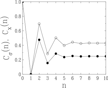
Figure 19: Plot of correlation functions for the cluster aggregation model of Refs. [56, 57] against the distance $n$ along the chain. Empty symbols: correlation $C_{\sigma}(n)$ of the survival index. Full symbols: correlation $C_{x}(n)$ of the reduced mass.

In conclusion, we emphasise that Edwards’ flatness in the landscape of configurational entropies is not the generic fate of strongly nonequilibrium models with slow dynamics, even when they have many features in common. The similarity between our column model [9] and the random graphs model [8] discussed in the previous section is thus all the more remarkable; both models manifest Edwards’ flatness in the jamming limit, deviating from it whenever free volume constraints are relaxed.

5.4 Low-temperature dynamics along the column: intermittency

We now return to the investigation of the column model [9], to do with its low-temperature dynamics. For rational $\varepsilon$, the presence of a finite but low shaking intensity merely increases the magnitude of density fluctuations [30], given that the zero-temperature dynamics is in any case stochastic. However, for irrational $\varepsilon$, low-temperature dynamics introduces an intermittency in the position of a surface layer; this has recently been observed in experiments on vibrated granular beds [58].

This happens as follows: when the shaking amplitude $\Gamma$ is such that it does not distinguish between a very small void $h_{n}$ and the strict absence of one, the site $n$ ‘looks like’ a point of perfect packing. The grain at depth $n$ then has the freedom to point the ‘wrong’ way; we call such sites excitations, using the thermal analogy. The probability of observing an excitation at site $n$ scales as $\Pi(n)\approx\exp(-2|h_{n}|/\Gamma)$. The uppermost site $n$ such that $|h_{n}|\sim\Gamma\ll 1$ will be the ’preferred’ excitation; it is propagated ballistically (cf. zero-temperature irrational $\varepsilon$ dynamics) until another excitation is nucleated above it. Its instantaneous position ${\cal N}(t)$ denotes the layer at which shape effects are lost in thermal noise, i.e., it separates an upper region of quasiperiodic ordering from a lower region of density fluctuations (5.4).

Fig. 20 shows a typical sawtooth plot of the instantaneous depth ${\cal N}(t)$, for a temperature $\Gamma=0.003$. The ordering length, defined as $\langle{\cal N}\rangle$, is expected to diverge at low temperature, as excitations become more and more rare; we find in fact [9] a divergence of the ordering length at low temperature of the form $\langle{\cal N}\rangle\sim 1/(\Gamma|\ln\Gamma|)$. This length is a kind of finite-temperature equivalent of the ‘zero-temperature’ length $\xi_{\rm dyn}$, as it divides an ordered boundary layer from a lower (bulk) disordered region. We emphasise once again that fast dynamics predominates in both zero-temperature and finite temperature boundary layers ($\xi_{\rm dyn}$ and $\langle{\cal N}\rangle$), with slow dynamics setting in for column depths beyond these.

Figure 20: Plot of the instantaneous depth ${\cal N}(t)$ of the ordered layer, for $\varepsilon=\Phi$ (the golden mean) and $\Gamma=0.003$. Dashed lines: leading nucleation sites given by Fibonacci numbers (bottom to top: $F_{11}=89$, $F_{12}=144$, $F_{13}=233$) (after [9]).

5.5 Discussion

We have discussed the effect of shape in granular compaction near the jamming limit, via a column model of grains [9]. Our main conclusions are that jagged (irregular) grains are characterised by optimal ground states, which are easily retrievable, while smooth (regular) grains cannot retrieve their ground states of perfect packing; in the latter case, even zero-temperature dynamics results in density fluctuations. We predict also that grain irregularities result in a surface intermittency for low-amplitude shaking, in agreement with recent experimental observations [58].

6 Conclusions

We have here reviewed some of our approaches to granular dynamics, now well known to consist of both fast and slow relaxational processes [1]. In the first case, grains typically compete with each other, while in the second, they cooperate. The dynamics of bridge formation is a typical result of cooperation, as is the relaxation of the angle of repose; competition between density fluctuations and external driving forces can, on the other hand, result in sandpile collapse. In the random graphs model presented above, the SPRT density separates regions of cooperation and competition, each with its own distinctive features. Finally, while slow dynamics predominate deep inside our column model of compacting grains, fast dynamics gives rise to strikingly rough configurational landscapes and surface intermittency.

References

References

- [1] Mehta,A., in Granular Matter: An Interdisciplinary Approach, 1994 ed. Mehta, A., (Springer, New York).
- [2] Mézard M, Parisi G, and Virasoro M A, 1987, Spin Glass Theory and Beyond (World Scientific, Singapore).
- [3] Marinari E, Parisi G, Ricci-Tersenghi F, and Zuliani F, 2001, J. Phys. A 34, 383; Mézard M, Physica A 2002 306, 25; Biroli G and Mézard M, 2002, Phys. Rev. Lett. 88, 025501; Lawlor A, Reagan D, McCullagh G D, De Gregorio P, Tartaglia P, and Dawson K A, 2002, Phys. Rev. Lett. 89, 245503.
- [4] see, e.g. Challenges in Granular Physics edited by Mehta A and Halsey T C, 2003, (Singapore: World Scientific); H M Jaeger H M, Nagel S R and Behringer R P, 1996, Rev. Mod. Phys. 68 1259; de Gennes P G 1999, Rev. Mod. Phys. 71 S374.
- [5] Mehta A, Barker G C, and Luck J M 2004 JSTAT P10014
- [6] Brown R L and Richards J C 1966 Principles of Powder Mechanics (Oxford: Pergamon)
- [7] Luck J M and Mehta A 2004 JSTAT (2004) P10015
- [8] Berg J and Mehta A 2001 Europhys. Lett. 56 784 —–2002 Phys. Rev. E 65, 031305.
- [9] Luck J M and Mehta A 2003 J. Phys. A 36 L365 —–2003 Eur. Phys. J. B 35 399
- [10] Mehta A and Barker G C 1991 Phys. Rev. Lett. 67 394 Barker G C and Mehta A 1992 Phys. Rev. A 45 3435 Barker G C and Mehta A 1993 Phys. Rev. E 47, 184
- [11] Edwards S F 1998 Physica 249 226
- [12] Silbert L E et al2002 Phys. Rev. E 65 031304
- [13] Donev A et al2004 Science 303 990
- [14] Edwards, S. F., 1994 in Granular Matter: An Interdisciplinary Approach, ed. Mehta, A., (Springer, New York).
- [15] Doi M and Edwards S F 1986 The Theory of Polymer Dynamics (Oxford: Clarendon)
- [16] To K, Lai P Y, and Pak H K 2001 Phys. Rev. Lett. 86 71
- [17] Liu C H et al1995 Science 269 513 Mueth D M, Jaeger H M, and Nagel S R 1998 Phys. Rev. E 57 3164
- [18] Erikson J M et al2002 Phys. Rev. E 66 040301 O’Hern C S et al2002 Phys. Rev. Lett. 88 075507
- [19] see chapters by Fukushima E and Seidler G T et al2003 in Challenges in Granular Physics edited by Mehta A and Halsey T C (Singapore: World Scientific)
- [20] Mehta A, Luck J M, and Needs R J 1996 Phys. Rev. E 53 92 Hoyle R B and Mehta A 1999 Phys. Rev. Lett. 83 5170
- [21] Uhlenbeck G E and Ornstein L S 1930 Phys. Rev. 36 823 Wang M C and Uhlenbeck G E 1945 Rev. Mod. Phys. 17 323
- [22] Bagnold R A 1966 Proc. R. Soc. London Ser. A 295 219
- [23] Mehta A and Barker G C 2001 Europhys. Lett. 56 626
- [24] Daerr A and Douady S 1999 Nature 399 241
- [25] Edwards S F 1998 Physica 249 226
- [26] Reynolds O 1885 Phil. Mag. 20 469
- [27] Nagel S R 1992 Rev. Mod. Phys. 64 321
- [28] Jaeger H M, Liu C H, and Nagel S R 1989 Phys. Rev. Lett. 62 40
- [29] Smoluchowski M V 1916 Z. Phys. 17 557
- [30] Nowak, E.R., Knight,J.B., Povinelli, M., Jaeger, H.M and Nagel, S.R., 1997 Powder Technology 94, 79. Nowak, E.R., Knight,J.B., Ben-Naim, E., Jaeger, H.M and Nagel, S.R., 1998 Phys. Rev. E 57, 1971.
- [31] Mehta, A., and Barker, G. C., 1994 Europhys. Lett. 27, 501. Stadler, P. F., Luck, J. M., and Mehta, A., 2002 Europhys. Lett.57, 46.
- [32] Caglioti, E., Loreto, V., Herrmann, H. J., and Nicodemi, M., 1997 Phys. Rev. Lett. 79, 1575.
- [33] Kurchan, J., 2000 J. Phys. Cond. Mat, 12, 6611.
- [34] B. Bollobas, Random Graphs (Academic Press, London, 1985)
- [35] Kob, W., and Andersen, H.C., 1993 Phys. Rev. E 48, 4364.
- [36] Ricci-Tersenghi, F., Weigt, M., and Zecchina, R., 2001 Phys. Rev. E 63, 026702.
- [37] Newman, M., and Moore,C., 1999 Phys Rev.E60, 5068.
- [38] Mehta, A., and Barker, G. C., 2000 J. Phys - Cond. Mat.12, 6619. Barker, G. C., and Mehta, A., 2002 Phase Transitions, 75, 519.
- [39] Villarruel, F. X., Lauderdale, B. E., Mueth, D. E., and Jaeger, H. E., 2000 Phys. Rev. E 61, 6914.
- [40] Dean, A. S., and Lefèvre, A., 2001 Phys. Rev. Lett. 86, 5639.
- [41] Even in the presence of frustration, a blocked state can be suitably defined: it merely implies that the grain is aligned with its net local field, i.e., it is connected to more unfrustrated than frustrated clusters.
- [42] Weeks, E. R., Crocker, D. E., Levitt, A. C., Schofield, A., and Weitz, D. A., 2002 Science 287, 627.
- [43] Nowak, E. R., Grushin, A., Barnum, A. C. B., and Weissman, M. B., 2001 Phys. Rev. E 63, 020301.
- [44] Barrat, A., and Zecchina, R., 1999 Phys. Rev. E 59 R1299.
- [45] Bernal, J. D., 1964 Proc. R. Soc. London A280, 299.
- [46] Monasson, R., 1995 Phys. Rev. Lett.75,2847.
- [47] Franz, S., and Parisi, G., 1995 J. Physique 5,1401.
- [48] Kolan, A. J., Nowak E. R.,and Tchakenko, A. J.,1999 Phys. Rev.E 59 3094.
- [49] Coniglio A. and Nicodemi M., 2000 J. Phys C 12 6601.
- [50] Liu A. J,. and Nagel, S. R., 1998 Nature 396, 21.
- [51] Biswas, P., Majumdar, A., Mehta, A., and Bhattacharjee, J. K., 1998 Physical Review E58, 1266.
- [52] Despite the use of very low ramp rates and large ’equilibration times’ at each tap, ’jamming’ at densities lower than was not observed in [31, 38, 49]; on the contrary, the results of all these simulations implied that the asymptotic density of random close packing would always be approached in the limit of sufficiently low ramp rates.
- [53] Berg J., and Mehta A., 2003 in Challenges in Granular Physics edited by Mehta A and Halsey T C (Singapore: World Scientific)
- [54] Monasson R., and Pouliquen, O., 1997 Physica A 236, 395.
- [55] Majumdar, A. S., Mehta, A., and Luck, J. M., 2005 Physics Letters B 607, 219.
- [56] Luck, J. M., and Mehta, A., cond-mat/0410385, 2005, to appear in Eur. Phys. J. B
- [57] Mehta, A., cond-mat/0411684.
- [58] Caballero, G., Lindner, A., Ovarlez, G., Reydellet, G., Lanuza, J., and Clement, E., 2004 in Unifying Concepts in Granular Media and Glasses edited by Coniglio, A., Fierro, A., Herrmann, H. J., and Nicodemi, M. (Elsevier).