Variational Perturbation Theory for Fokker-Planck Equation with Nonlinear Drift

Abstract

We develop a recursive method for perturbative solutions of the Fokker-Planck equation with nonlinear drift. The series expansion of the time-dependent probability density in terms of powers of the coupling constant is obtained by solving a set of first-order linear ordinary differential equations. Resumming the series in the spirit of variational perturbation theory we are able to determine the probability density for all values of the coupling constant. Comparison with numerical results shows exponential convergence with increasing order.

I INTRODUCTION

In many problems of physics, chemistry and biology one has to deal with vast numbers of influences which are not fully known and are thus modelled by noise or fluctuations Gardiner ; Stratonovich ; Kampen ; Haken1 . The stochastic approach to such systems identifies some relevant macroscopic property $x$ governed by a drift coefficient $K(x)$, while the microscopic degrees are averaged to noise, entering as a stochastic force. In the case of additive noise this simply leads to a diffusion constant $D$. Thus we arrive at the Fokker-Planck equation (FP) Risken for the density $\mathcal{P}(x,t)$ of the probability to find the system in a state with property $x$ at time $t$:

$$\dfrac{\partial}{\partial t}\mathcal{P}(x,t)=-\frac{\partial}{\partial x}\left[K(x)\mathcal{P}(x,t)\right]+D\frac{\partial^{2}}{\partial x^{2}}\mathcal{P}(x,t)\,.$$ (1)

Once $\mathcal{P}(x,t)$ is known from solving (1), we can calculate the ensemble average of any function $\mathcal{O}(x)$ according to

$$\langle\mathcal{O}(x(t))\rangle=\int_{-\infty}^{+\infty}\mathcal{O}(x(t))\mathcal{P}(x,t)\,dx\,.$$ (2)

In this paper we consider a stochastic model with the nonlinear drift coefficient

$$K(x)=-\gamma\,x-gx^{3}\,.$$ (3)

Such models are studied, for instance, in semiclassical treatments of a laser near to its instability threshold Risken ; Haken3 , where the variable $x$ is taken to be the electric field. The damping constant $\gamma$ is set proportional to the difference between the pump parameter $\sigma$ and its threshold value $\sigma_{\rm thr}$, so that the laser instability corresponds to $\gamma=0$. The coupling constant $g\geq 0$ describes the interaction between light and matter within the dipole approximation, and the diffusion constant $D$ in the FP equation characterizes the spontaneous emission of radiation. While the linear case with $g=0$, corresponding to Brownian motion with damping constant $\gamma$, can be solved analytically, there is no exact solution for the nonlinear case with $g>0$. But we can find a solution in form of a series expansion of the probability density $\mathcal{P}(x,t)$ in powers of the coupling constant $g$. This series is asymptotic, i.e. its expansion coefficients increase factorially with the perturbative oder and alternate in sign.

Such divergent weak-coupling series are known from various fields of physics, e.g. quantum statistics or critical phenomena, and resummation techniques have been invented to extract meaningful information in such situations. Powerful tools among them are the variational methods, independently studied by many groups. (see e.g. the references in HampKleinert1 ). A simple example is the so-called $\delta$-expansion of the anharmonic quantum oscillator, where the trial frequency of an artificial harmonic oscillator introduced to maximally counterbalance the nonlinear term, is optimized following the principle of minimal sensitivity Stevenson . It turns out that the $\delta$-expansion procedure corresponds to a systematic extension of a variational approach in quantum statistics Feynman1 ; Feynman2 ; Tognetti1 ; Tognetti2 to arbitrary orders as developed by Kleinert Kleinertsys ; Festschrift ; Kleinert , now being called variational perturbation theory (VPT). In recent years, VPT has been extended in a simple but essential way to also allow for the resummation of divergent perturbation expansions which arise from renormalizing the $\phi^{4}$-theory of critical phenomena Festschrift ; KleinertD1 ; KleinertD2 ; Verena . The most important new feature of this field-theoretic variational perturbation theory is that it accounts for the anomalous power approach to the strong-coupling limit which the $\delta$-expansion cannot do. This approach is governed by an irrational critical exponent as was first shown by Wegner Wegner in the context of critical phenomena. In contrast to the $\delta$-expansion, the field-theoretic variational perturbation expansions cannot be derived from adding and subtracting a harmonic term. Instead, a self-consistent procedure is set up to determine this irrational critical Wegner exponent. The theoretical results of the field-theoretic variational perturbation theory are in excellent agreement with the only experimental value available so far with appropriate accuracy, the critical exponent $\alpha$ governing the behaviour of the specific heat near the superfluid phase transition of ⁴He which was measured in a satellite orbiting around the earth Festschrift ; Verena ; Satellit ; Lipa .

Recently, the VPT techniques have been applied to Markov theory, approximating a nonlinear stochastic process by an effective Brownian motion Putz ; Okopinska . This is achieved by adding and subtracting a linear term to the nonlinear drift coefficient (3), where the new damping constant is taken as the variational parameter. In the present paper we extend this result to higher orders, which we have made accessible by our recursive approach Dreger . By doing so, we are able to show that VPT makes Markov theory converge exponentially with respect to order, a phenomenon known for various other systems Janke1 ; Janke2 ; Guida ; Proof ; Kuerzinger ; Weissbach ; Schanz .

The paper is structured as follows. In Sec. II we review some properties of the FP equation which are essential for our discussion. In Sec. III we present the asymptotic perturbation expansion for the normalization constant of the stationary solution of the FP equation with the drift coefficient (3) and its variational resummation. This simple case already illustrates in an introductory fashion all features of the upcoming treatment of the time-dependent problem. In Sec. IV we perturbatively solve the FP equation with a nonlinear drift coefficient (3) for Gaussian initial distributions by means of a double expansion with respect to the coupling strength $g$ and the variable $x$. In Sec. V we apply VPT to the resulting divergent weak-coupling expansion of the probability density to render the results convergent for all values of the coupling constant $g$. Furthermore, we discuss the exponential convergence of our variational method with respect to the order. The paper closes with a summary in Sec.VI.

II FOKKER-PLANCK EQUATION

In this section we fix our notation by reviewing the main properties of one-dimensional stochastic Markov processes.

II.1 Definitions

A stochastic Markov process $x(t)$ is described by an ordinary stochastic differential equation which is of the Langevin form

$$\dot{x}(t)=a(x(t))+b(x(t))\,\Gamma(t)\,,$$ (4)

where $\Gamma(t)$ is a Gaussian distributed stochastic force with zero mean and $\delta$-correlation:

$$\langle\Gamma(t)\rangle=0,\qquad\langle\Gamma(t)\Gamma(t^{\prime})\rangle=2\delta(t-t^{\prime})\,.$$ (5)

For the special case of the coefficient $b(x)\equiv b$ being constant, the stochastic system is said to be driven by additive noise, and the time evolution of its probability density $\mathcal{P}(x,t)$ is described by the Fokker-Planck equation (1) with drift coefficient $K(x)=a(x)$ and diffusion coefficient $D=b^{2}$ Risken . The FP equation (1) has the form of a continuity equation

$$\frac{\partial}{\partial t}\mathcal{P}(x,t)+\frac{\partial}{\partial x}\mathcal{S}(x,t)=0$$ (6)

with probability current

$$\mathcal{S}(x,t)=K(x)\mathcal{P}(x,t)-D\frac{\partial}{\partial x}\mathcal{P}(x,t)\,.$$ (7)

For natural boundary conditions, where $\mathcal{S}(x,t)\to 0$ as $x\to\pm\infty$, probability conservation is thus guaranteed:

$$\frac{\partial}{\partial t}\int_{-\infty}^{+\infty}dx\,\mathcal{P}(x,t)=0\,.$$ (8)

In the case of additive noise, the drift coefficient $K(x)$ can be derived from a potential

$$\Phi(x)=-\frac{1}{D}\int^{x}K(y)\,dy$$ (9)

such that

$$K(x)=-D\,\Phi^{\prime}(x)\,.$$ (10)

If the potential satisfies $\Phi(x)\to+\infty$ for $x\to\pm\infty$, the probability density $\mathcal{P}(x,t)$ approaches a stationary values $\mathcal{P}_{\text{stat}}(x)$ in the long-time limit, i.e.

$$\mathcal{P}_{\text{stat}}(x)=\lim_{t\to\infty}\mathcal{P}(x,t)=\mathbf{N}\,e^{-\Phi(x)}\,,$$ (11)

where the normalization constant $\mathbf{N}$ is found to be

$$\mathbf{N}=\left\{\int_{-\infty}^{+\infty}\exp\left[\frac{1}{D}\int^{x}K(y)\,dy\right]dx\right\}^{-1}\,.$$ (12)

II.2 Brownian Motion

For Brownian motion, defined by a linear drift coefficient

$$K(x)=-\gamma\,x$$ (13)

with damping $\gamma>0$, we have a harmonic potential:

$$\Phi(x)=\dfrac{\gamma}{2D}x^{2}$$ (14)

and the FP equation (1) has a solution in closed form. With initial condition

$$\mathcal{P}(x,x_{0};0)=\delta(x-x_{0})$$ (15)

the solution is

$$\mathcal{P}(x,x^{\prime};t) = \sqrt{\frac{\gamma}{2\pi D(1-e^{-2\gamma\,t})}}$$ (16)

$$\times\exp\!\left[-\frac{(x-x^{\prime}e^{-\gamma\,t})^{2}}{2D(1-e^{-2\gamma\,t})/\gamma}\right]\,.$$

It represents the Green function of the FP equation with the drift coefficient (13), describing the evolution of the probability density starting with an arbitrary initial distribution according to

$$\mathcal{P}(x,t)=\int_{-\infty}^{+\infty}\mathcal{P}(x,x^{\prime};t-t^{\prime})\mathcal{P}(x^{\prime},t^{\prime})dx^{\prime}\,.$$ (17)

For instance, the initial Gaussian probability density

$$\mathcal{P}(x;t=0)=\frac{1}{\sqrt{2\pi\sigma^{2}}}\exp\left[-\frac{(x-\mu)^{2}}{2\sigma^{2}}\right]$$ (18)

has the time evolution

$$\mathcal{P}_{\gamma}(x,t) = \sqrt{\frac{\gamma}{2\pi[D-(D-\gamma\sigma^{2})e^{-2\gamma t}]}}$$ (19)

$$\times\exp\!\left[-\frac{\gamma}{2}\frac{(x-\mu\,e^{-\gamma t})^{2}}{D-(D-\gamma\sigma^{2})e^{-2\gamma t}}\right]\,.$$

In the long-time limit it approaches the stationary distribution

$$\mathcal{P}_{\text{stat}}(x)=\lim_{t\to\infty}\mathcal{P}_{\gamma}(x,t)=\sqrt{\frac{\gamma}{2\pi D}}\exp\left(-\frac{\gamma\,x^{2}}{2D}\right)$$ (20)

which turns out to be independent of the parameters $\mu$ and $\sigma$ of the initial distribution (18).

II.3 Nonlinear Drift

Consider now an additional nonlinear drift (3) so that the potential (9) becomes

$$\Phi(x)=\frac{\gamma}{2D}x^{2}+\frac{g}{4D}x^{4}\,.$$ (21)

While there exists no closed solution of the corresponding FP equation (1)

$$\frac{\partial}{\partial t}\mathcal{P}(x,t)=\frac{\partial}{\partial x}\left[(\gamma x+gx^{3})\mathcal{P}(x,t)\right]+D\frac{\partial^{2}}{\partial x^{2}}\mathcal{P}(x,t)\,,$$ (22)

its stationary distribution (11) is given by

$$\mathcal{P}_{\text{stat}}(x)=\mathbf{N}(g)\exp\left(-\frac{\gamma}{2D}x^{2}-\frac{g}{4D}x^{4}\right)$$ (23)

with normalization constant

$$\mathbf{N}(g)=\left[\int_{-\infty}^{+\infty}\exp\left(-\frac{\gamma}{2D}x^{2}-\frac{g}{4D}x^{4}\right)dx\right]^{-1}\,.$$ (24)

Performing the integral in (24), we obtain

$$\mathbf{N}(g)=\begin{cases}\sqrt{\frac{2g}{\gamma}}\exp\left(-\tfrac{\gamma^{2}}{8Dg}\right)\Bigl{/}\mathrm{K}_{1/4}\left(\tfrac{\gamma^{2}}{8Dg}\right)&\text{; $\gamma>0$\, ,}\\[8.5359pt] \left(\frac{4g}{D}\right)^{1/4}\Bigl{/}\Gamma\left(\frac{1}{4}\right)&\text{; $\gamma=0$\, ,}\\[4.26773pt] \frac{\frac{2}{\pi}\sqrt{\frac{g}{|\gamma|}}\exp\left(-\tfrac{\gamma^{2}}{8Dg}\right)}{\left[\mathrm{I}_{-1/4}\left(\tfrac{\gamma^{2}}{8Dg}\right)+\mathrm{I}_{1/4}\left(\tfrac{\gamma^{2}}{8Dg}\right)\right]}&\text{; $\gamma<0$\,,}\end{cases}$$ (25)

where $\mathrm{I}_{\nu}(z)$ and $\mathrm{K}_{\nu}(z)$ denote modified Bessel functions of $\nu$-th order of first and second kind, respectively Gradshteyn .

$n$	$\sqrt{2\pi}\,a_{n}$	$b_{n}$
0	$1$	$0.390\,062\,251\,089\,407=\Gamma(3/4)/\pi$
1	$3/4$	$0.131\,836\,797\,004\,050\,253\,244$
2	$-87/32$	$-0.004\,198\,378\,378\,722\,963\,623$
3	$2889/128$	$-0.001\,419\,006\,213\,792\,844\,574$
4	$-581157/2048$	$0.000\,536\,178\,450\,689\,882\,683$
5	$38668509/8192$	$-0.000\,093\,437\,511\,028\,762\,876$

Table 1: The first 6 coefficients of the weak- and strong-coupling expansion (26) and (29), respectively, for $D=\gamma=1$.

III NORMALIZATION CONSTANT

The diverging behaviour of a perturbation series as well as the method of VPT to overcome this problem can already be studied by considering the normalization constant (24) of the stationary solution (23). To simplify our discussion we assume in this section without loss of generality $D=1$.

III.1 Weak- and Strong-Coupling Expansion

The weak-coupling expansion

$$\mathbf{N}_{\text{weak}}^{(N)}(g)=\sum_{n=0}^{N}a_{n}\,g^{n}$$ (26)

follows from (24) by expanding the $\exp(-gx^{4}/4)$-term in the integrand:

$$\mathbf{N}_{\text{weak}}^{(N)}(g)=\left[\sqrt{2}\sum_{k=0}^{N}\frac{(-g)^{k}}{k!}\frac{\Gamma(1/2+2k)}{\gamma^{1/2+2k}}\right]^{-1}\,.$$ (27)

On the other hand, a rescaling $x\to(4/g)^{1/4}y$ in the normalization integral (24) leads to

$$\mathbf{N}(g)=\left(\frac{g}{4}\right)^{1/4}\left[\int_{-\infty}^{+\infty}\exp\left(-\frac{\gamma}{g^{1/2}}y^{2}-y^{4}\right)dy\right]^{-1}\,,$$ (28)

so the strong-coupling expansion

$$\mathbf{N}_{\text{strong}}^{(M)}(g)=g^{1/4}\sum_{m=0}^{M}b_{m}\,g^{-m/2}$$ (29)

follows from (28) by expanding the term $\exp(-\gamma y^{2}/g^{1/2})$ in the integrand

$$\mathbf{N}_{\text{strong}}^{(M)}(g)=\left(\frac{g}{4}\right)^{1/4}\left[\sum_{k=0}^{M}\frac{(-\gamma)^{k}}{g^{k/2}}\frac{\Gamma(1/4+k/2)}{2k!}\right]^{-1}.$$ (30)

Note that the weak-coupling expansion (26) contains integer powers of $g$, whereas dimensional arguments lead to rational powers of $g$ for the strong-coupling expansion (29). The first six coefficients $a_{n},b_{m}$ are given in Table 1 and the respective expansions (26) and (29) are depicted in Figure 1. While the weak-coupling expansion provides good results for small values of $g$, the strong-coupling expansion describes the behavior for large values of $g$. For intermediate values of $g$ both series yield poor results.

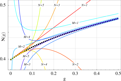
Figure 1: Weak- and strong-coupling expansions (26) and (29) up to the $5$th order, respectively, as well as the exact normalization constant (24) ($\bullet\,\bullet\,\bullet$) for $D=\gamma=1$.

III.2 Variational Perturbation Theory

Despite its diverging nature, all information on the analytic function $\mathbf{N}(g)$ is already contained in the weak-coupling expansion (26). One way to extract this information and use it to render the series convergent for any value of the coupling constant $g$ is provided by VPT as developed by Kleinert Verena ; Festschrift ; Kleinert . This method is based on introducing a dummy variational parameter on which the full perturbation expansion does not depend, while the truncated expansion does. The optimal variational parameter is then selected by invoking the principle of minimal sensitivity Stevenson , requiring the quantity of interest to be stationary with respect to the variational parameter. In our context Putz ; Okopinska ; Dreger , this dummy variational parameter can be thought of as the damping constant $\kappa$ of a trial Brownian motion with a harmonic potential $\kappa x^{2}/2$, which is tuned in such a way, that it effectively compensates the nonlinear potential. In order to introduce the variational parameter $\kappa$, we add the harmonic potential $\kappa x^{2}/2$ of the trial Brownian motion to the nonlinear potential (21) and subtract it again:

$$\Phi(x)=\frac{\kappa}{2}x^{2}+\frac{g}{4}x^{4}+\frac{\gamma-\kappa}{2}x^{2}\,.$$ (31)

By doing so, we consider the harmonic potential $\kappa x^{2}/2$ as the unperturbed term and treat all remaining potential terms in (31) as a perturbation. Such a formal perturbation expansion is performed for the normalization constant (24) according to

$$\mathbf{N}(g) = \left\{\int_{-\infty}^{+\infty}\exp\Bigg{[}-\frac{\kappa}{2}x^{2}\right.$$ (32)

$$\left.\left.-\delta\left(\frac{g}{4}x^{4}+\frac{\gamma-\kappa}{2}x^{2}\right)\Bigg{]}dx\right\}^{-1}\right|_{\delta=1}\,,$$

where the additional parameter $\delta$ is introduced in the spirit of the $\delta$-expansion (see, for instance, the references in HampKleinert1 ). Due to the rescaling $x\to\tilde{x}/\beta(\delta)$ with the scaling factor

$$\beta(\delta)=\sqrt{[\kappa+\delta(\gamma-\kappa)]/\gamma}\,,$$ (33)

the weak-coupling expansion (26) of (24) leads to:

$$\mathbf{N}(g)=\left.\beta(\delta)\sum_{n=0}^{\infty}a_{n}\left[\frac{\delta g}{\beta^{4}(\delta)}\right]^{n}\right|_{\delta=1}\,.$$ (34)

Expanding and truncating the series at order $N$ in $\delta$, we obtain the $N$th variational approximation to the normalization constant $\mathbf{N}(g)$:

$$\mathbf{N}_{\text{VPT}}^{(N)}(g,\kappa) = \sum_{n=0}^{N}a_{n}\left(\frac{\kappa}{\gamma}\right)^{1/2-2n}g^{n}$$ (37)

$$\times\sum_{k=0}^{N-n}\left(\begin{array}[]{c}1/2-2n\\ k\end{array}\right)\left(\frac{\gamma-\kappa}{\kappa}\right)^{k}\,.$$

Equivalently, the variational expression (37) also follows directly from the weak-coupling expansion (26). To this end we remark that, due to dimensional arguments, the respective coefficients depend via

$$a_{n}=\tilde{a}_{n}\,\gamma^{1/2-2n}$$ (38)

on $\gamma$ where $\tilde{a}_{n}$ denote dimensionless quantities. Treating in (31) the harmonic potential $\kappa x^{2}/2$ as the unperturbed term and all remaining potential terms as a perturbation, corresponds then to the substitution

$$\gamma\to\kappa(1+gr)$$ (39)

with the abbreviation

$$r=\frac{\gamma-\kappa}{\kappa g}\,.$$ (40)

Thus inserting (39) in the weak-coupling expansion (26), (38), a reexpansion in powers of $g$ up to order $N$ together with the resubstitution (40) leads to a rederivation of (37).

As the normalization constant $\mathbf{N}(g)$ does not depend on the variational parameter $\kappa$, it is reasonable to ask for the truncated series (37) to depend on $\kappa$ as little as possible. Therefore, we invoke the principle of minimal sensitivity Stevenson and demand

$$\left.\frac{\partial}{\partial\kappa}\mathbf{N}_{\text{VPT}}^{(N)}(g,\kappa)\right|_{\kappa=\kappa_{\text{opt}}^{(N)}(g)}=0\,.$$ (41)

The optimal variational parameter $\kappa_{\text{opt}}^{(N)}(g)$ leads to the $N$th order variational approximation $\mathbf{N}_{\text{VPT}}^{(N)}(g,\kappa_{\text{opt}}^{(N)}(g))$ to the normalization constant $\mathbf{N}(g)$. In case that (41) is not solvable, we determine $\kappa_{\text{opt}}^{(N)}(g)$ from the zero of the second derivative in accordance with the principle of minimal sensitivity Stevenson :

$$\left.\frac{\partial^{2}}{\partial\kappa^{2}}\mathbf{N}_{\text{VPT}}^{(N)}(g,\kappa)\right|_{\kappa=\kappa_{\text{opt}}^{(N)}(g)}=0\,.$$ (42)

If it happens that (41) or (42) have more than one solution, we select that particular one which is closest to the solution in the previous variational order.

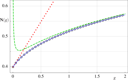
Figure 2: First-oder variational result (—) compared with exact normalization constant $(\circ\circ\circ)$. First-order weak- and strong-coupling approximations are shown by dashed (– –) and dotted ($\cdot\!\cdot\!\cdot$) lines, respectively.

As an illustrative example we treat explicitly the first variational order where we obtain

$$\mathbf{N}_{\text{VPT}}^{(1)}(g,\kappa)=\frac{2\kappa(\kappa+\gamma)+3g}{4\sqrt{2\pi\kappa^{3}}}\,,$$ (43)

so that the first derivative with respect to $\kappa$

$$\frac{\partial}{\partial\kappa}\mathbf{N}^{(1)}_{\text{vpt}}(g,\kappa)=\frac{2\kappa(\kappa-\gamma)-9g}{8\sqrt{2\pi\kappa^{5}}}$$ (44)

has the two zeros

$$\kappa_{\text{opt}}^{(1,\pm)}(g)=\frac{1}{2}\left(\gamma\pm\sqrt{18g+\gamma^{2}}\,\right).$$ (45)

Since the variational parameter has to approach $\gamma$ for a vanishing coupling constant $g$, we select from (45) the solution $\kappa_{\text{opt}}^{(1,+)}(g)$. The resulting optimized result $\mathbf{N}_{\text{VPT}}^{(1)}(g,\kappa_{\text{opt}}^{(1,+)}(g))$ is shown in Figure 2. We observe that in this parameter range already the first-order variational approximation $\mathbf{N}_{\text{VPT}}^{(1)}(g,\kappa_{\text{opt}}^{(1,+)}(g))$ is indistinguishable from the exact normalization constant $\mathbf{N}(g)$.

III.3 Exponential Convergence

In order to quantify the accuracy of the variational approximations, we study now, in particular, the strong-coupling regime $g\to\infty$. In first order, the insertion of (45) in (43) leads to the strong-coupling expansion (29) with the leading coefficient

$$b_{0}^{(1)}=\left(\frac{2}{9\pi^{2}}\right)^{1/4}\approx 0.387\,.$$ (46)

Comparing (46) with $b_{0}=\Gamma(3/4)/\pi\approx 0.390$ (see Table 1), we conclude that first-order variational perturbation theory yields the leading strong-coupling coefficient within an accuracy of less than 1 %.

To obtain higher-order variational results for this strong-coupling coefficient $b_{0}$, we proceed as follows. From the first-order approximation (45) we see that the variational parameter has a strong-coupling expansion $\kappa^{(1,+)}_{\rm opt}(g)=\sqrt{g}\,3\sqrt{2}/2+\ldots$, whose form turns out to be valid also for the orders $N>1$. Inserting the ansatz $\kappa^{(N)}_{\rm opt}(g)=\kappa_{0}^{(N)}\sqrt{g}+\ldots$ in (37), we obtain the $N$th order approximation for the leading strong-coupling coefficient $b_{0}$:

$$b_{0}^{(N)}(\kappa_{0}^{(N)}) = \sum_{n=0}^{N}a_{n}\left(\frac{\kappa_{0}^{(N)}}{\gamma}\right)^{1/2-2n}$$ (49)

$$\times\sum_{k=0}^{N-n}\left(\begin{array}[]{@{}c}1/2-2n\\ k\end{array}\right)\,(-1)^{k}\,.$$

The inner sum can be performed explicitly by using Eq. (0.151.4) in Ref. Gradshteyn :

$$b_{0}^{(N)}(\kappa_{0}^{(N)})=\sum_{n=0}^{N}(-1)^{N-n}\,\left(\begin{array}[]{@{}c}-1/2-2n\\ N-n\end{array}\right)a_{n}\left(\frac{\kappa_{0}^{(N)}}{\gamma}\right)^{1/2-2n}.$$ (52)

In order to optimize (52) we look again for an extremum

$$\frac{\partial b_{0}^{(N)}(\kappa_{0}^{(N)})}{\partial\kappa_{0}^{(N)}}=0$$ (53)

or for a saddle point

$$\frac{\partial^{2}b_{0}^{(N)}(\kappa_{0}^{(N)})}{\partial\kappa_{0}^{(N)}{}^{2}}=0\,.$$ (54)

It turns out that extrema exist for odd orders $N$, whereas even orders $N$ lead to saddle points. The points of Figure 3 show the logarithmic plot of the relative error $|b^{(N)}_{0}(\kappa_{0}^{(N)})-b_{0}|/b_{0}$ when using the smallest zero of the first and second derivative, i.e. (53) and (54), respectively. We observe that the relative error depends linearily on $N^{1/2}$ up to the order $N=120$ according to

$$\frac{|b^{(N)}_{0}(\kappa_{0}^{(N)})-b_{0}|}{b_{0}}=e^{-\alpha-\beta\,N^{1/2}}\,,$$ (55)

where the fit to the straight line $-\alpha-\beta N^{1/2}$ leads to the quantities $\alpha=0.139714$ and $\beta=1.33218$. Thus we have demonstrated that the variational approximations for the leading strong-coupling coefficient converge exponentially fast. Note that the speed of convergence is faster than the exponential convergence of the variational results for the ground-state energy of the anharmonic oscillator Janke1 ; Janke2 .

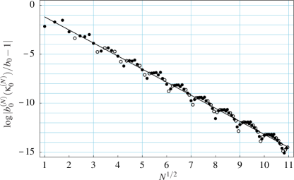
Figure 3: The points show the logarithmic plot of the relative error $|b^{(N)}_{0}(\kappa_{0}^{(N)})-b_{0}|/b_{0}$ when using the smallest zero of the first ($\bullet$) and the second derivative $(\circ)$, respectively, against $N^{1/2}$. The solid line represents a fit to the straight line $-\alpha-\beta N^{1/2}$.

IV RECURSION RELATIONS

Now we elaborate the perturbative solution of the FP equation (22) with the initial distribution (18). By doing so, we follow the notion of Ref. Weissbach and generalize the recursive Bender-Wu solution method for the Schrödinger equation of the anharmonic oscillator Bender , thus obtaining a recursive set of first-order ordinary differential equations Dreger .

IV.1 Time Transformation

At first we perform a suitable time transformation which simplifies the following calculations:

$$\tau(t)=\tau_{0}e^{-\gamma t}\,,\qquad\tau_{0}=\sqrt{1-\gamma\sigma^{2}/D}\,.$$ (56)

Thus the new time $\tau$ runs from $\tau_{0}$ to $0$ when the physical time $t$ evolves from $0$ to $\infty$. Due to (56) the FP equation (22) is transformed to

$$-\gamma\tau\frac{\partial}{\partial\tau}\mathcal{P}(x,\tau)=\frac{\partial}{\partial x}\left[(\gamma x+gx^{3})\mathcal{P}(x,\tau)\right]+D\frac{\partial^{2}}{\partial x^{2}}\mathcal{P}(x,\tau)\,.$$ (57)

Furthermore, the initial distribution (18) reads then

$$\mathcal{P}(x,\tau=\tau_{0})=\frac{1}{\sqrt{2\pi\sigma^{2}}}\exp\!\left[-\frac{(x-\mu)^{2}}{2\sigma^{2}}\right]$$ (58)

and contains $P(x,\tau=1)=\delta(x-\mu)$ as a special case in the limit $\sigma^{2}\to 0$.

IV.2 Expansion in Powers of $g$

If the coupling constant $g$ vanishes, the solution of the initial value problem (57), (58) follows from applying the time transformation (56) to (19), i.e.

$$\mathcal{P}_{\gamma}(x,\tau)=\sqrt{\frac{\gamma}{2\pi D(1-\tau^{2})}}\exp\!\left[-\frac{\gamma}{2D}\frac{(x-x_{0}\tau)^{2}}{1-\tau^{2}}\right]\,,$$ (59)

where we have introduced the abbreviation

$$x_{0}=\frac{\mu}{\sqrt{1-\gamma\sigma^{2}/D}}\,.$$ (60)

For a coupling constant $g>0$, we solve (57) by the ansatz

$$\mathcal{P}(x,\tau)=\mathcal{P}_{\gamma}(x,\tau)\,q(x,\tau)\,,$$ (61)

so that the remainder $q(x,\tau)$ fulfills the partial differential equation

$$-\gamma\tau\frac{\partial}{\partial\tau}q(x,\tau)=\left[3gx^{2}+\frac{\gamma gx^{4}-\gamma g\tau x_{0}x^{3}}{D(\tau^{2}-1)}\right]q(x,\tau)$$

$$+\left[\frac{\gamma(\tau^{2}+1)x-2\gamma\tau x_{0}}{\tau^{2}-1}+gx^{3}\right]\frac{\partial}{\partial x}q(x,\tau)+D\frac{\partial^{2}}{\partial x^{2}}q(x,\tau)\,.$$ (62)

Then we solve (62) by expanding $q(x,\tau)$ in a Taylor series with respect to the coupling constant $g$, i.e.

$$q(x,\tau)=\sum_{n=0}^{\infty}g^{n}\,q_{n}(x,\tau)\,,$$ (63)

where we set $q_{0}(x,\tau)=1$. Thus the expansion coefficients $q_{n}(x,\tau)$ obey the partial differential equations

$$-\gamma\,\tau\frac{\partial}{\partial\tau}q_{n}(x,\tau)=\left[3x^{2}+\frac{\gamma x^{4}-\gamma\,\tau x_{0}x^{3}}{D(\tau^{2}-1)}+\frac{\partial}{\partial x}\right]q_{n-1}(x,\tau)$$

$$+\frac{\gamma(\tau^{2}+2)x-2\gamma\,\tau x_{0}}{\tau^{2}-1}\frac{\partial}{\partial x}q_{n}(x,\tau)+D\frac{\partial^{2}}{\partial x^{2}}q_{n}(x,\tau)\,.$$ (64)

IV.3 Expansion in Powers of $x$

It turns out that the partial differential equations (64) are solved by expansion coefficients $q_{n}(x,\tau)$ which are finite polynomials in $x$:

$$q_{n}(x,\tau)=\sum_{k=0}^{M_{n}}\alpha_{n,k}(\tau)x^{k}\,.$$ (65)

Indeed, inserting the decomposition (65) in (64), we deduce that the highest polynomial degree is given by $M_{n}=4n$. Note that in case of $\mu=0$ the partial differential equations (64) are symmetric with respect to $x\to-x$, so that only even powers $x$ appear in (65). From (64) and (65) follows that the functions $\alpha_{n,k}(\tau)$ are determined from

$$\frac{\partial}{\partial\tau}\alpha_{n,k}(\tau)\,+\,\frac{k(\tau^{2}+1)}{\tau(\tau^{2}-1)}\alpha_{n,k}(\tau)=r_{n,k}(\tau)\,,$$ (66)

where the inhomogeneity is given by

$$r_{n,k}(\tau)=-\frac{k+1}{\gamma\,\tau}\alpha_{n-1,k-2}(\tau)-\frac{D(k+2)(k+1)}{\gamma\,\tau}\alpha_{n,k+2}(\tau)$$

$$+\frac{x_{0}\alpha_{n-1,k-3}(\tau)}{D(\tau^{2}-1)}-\frac{\alpha_{n-1,k-4}(\tau)}{D(\tau^{3}-\tau)}+\frac{2x_{0}(k+1)}{\tau^{2}-1}\alpha_{n,k+1}(\tau)\,.$$ (67)

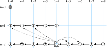
Figure 4: Recursive calculation of the functions $\alpha_{n,k}(\tau)$: $\alpha_{0,0}(\tau)=1$ is the only coefficient which is a priori nonzero (​). For each $n$ the coefficients are successively determined for $k=4n,\ldots,0$ (). Each step necessitates (​​) only those coefficients which are already known (​).

IV.4 Recursive Solution

The Eqs. (66) and (67) represent a system of first-order ordinary differential equations which can be recursively solved according to Figure 4. By doing so, one has to take into account $\alpha_{n,k}(\tau)=0$ if $n<0$ or $k<0$ or $k>4n$. The respective positions in the $(n,k)$-grid of Figure 4 are empty or lie outside. Iteratively calculating the coefficients $\alpha_{n,k}(\tau)$ in the $n$th order, we have to start with $k=4n$ and decrease $k$ up to $k=0$. In each iterative step the inhomogeneity (67) of (66) contains only those coefficients which are already known. The only coefficient which is a priori nonzero is $\alpha_{0,0}(\tau)=1$.

Applying the method of varying constants, the inhomogeneous differential equation (66) is solved by the ansatz

$$\alpha_{n,k}(\tau)=A_{n,k}(\tau)\,\frac{\tau^{k}}{(\tau^{2}-1)^{k}}\,,$$ (68)

where $A_{n,k}(\tau)$ turns out to be

$$A_{n,k}(\tau)=A_{n,k}(\tau_{0})+\int_{\tau_{0}}^{\tau}r_{n,k}(\sigma)\,\sigma^{-k}(\sigma^{2}-1)^{k}\,d\sigma\,.$$ (69)

The integration constant $A_{n,k}(\tau_{0})$ is fixed by considering the initial distribution (58). From (59), (61), (63), and (65) follows

$$1=1+\sum_{n=1}^{\infty}g^{n}\sum_{k=0}^{4n}\alpha_{n,k}(\tau_{0})x^{k}\,,$$ (70)

so we conclude $\alpha_{n,k}(\tau_{0})=0$ and thus $A_{n,k}(\tau_{0})=0$ for $n\geq 1$. Therefore, we obtain the final result

$$\alpha_{n,k}(\tau)=\frac{\tau^{k}}{(\tau^{2}-1)^{k}}\int_{\tau_{0}}^{\tau}r_{n,k}(\sigma)\,\sigma^{-k}(\sigma^{2}-1)^{k}\,d\sigma\,,$$ (71)

where $r_{n,k}(\sigma)$ is given by (67).

Note that the special case $\sigma^{2}\to 0$ with the initial distribution $P(x,\tau=1)=\delta(x-\mu)$ has to be discussed separately, as then (70) is not valid. In this case we still conclude for $k\neq 0$ that $A_{n,k}(\tau_{0}=1)=0$, otherwise $\alpha_{n,k}(\tau)$ in (68) would posses for $\tau=1$ a pole of order $k$. For $k=0$ this argument is not valid as the fraction in (68) is then no longer present. The integration constant $A_{n,0}(\tau_{0}=1)$ follows from considering the normalization integral of (61) for $\tau=1$ together with (63), and (65), i.e.

$$1=1+\sum_{n=1}^{\infty}g^{n}\sum_{k=0}^{4n}\alpha_{n,k}(\tau=1)x_{0}^{k}\,.$$ (72)

Indeed, taking into account (68) for $k=0$ leads to

$$A_{n,0}(\tau=1)=\alpha_{n,0}(\tau=1)=-\sum_{k=1}^{4n}\alpha_{n,k}(\tau=1)x_{0}^{k}\,.$$ (73)

Thus for $k\neq 0$ the coefficients $\alpha_{n,k}(\tau)$ are still given by (71), whereas for $k=0$ we obtain

$$\alpha_{n,0}(\tau)=\int_{1}^{\tau}\!r_{n,0}(\sigma)\,d\sigma-\sum_{k=1}^{4n}\alpha_{n,k}(\tau=1)x_{0}^{k}\,.$$ (74)

IV.5 Cumulant Expansion

The weak-coupling expansion (61), (63) of the probability density $\mathcal{P}(x,\tau)$ has the disadvantage that its truncation to a certain order $N$ could lead to negative values. To avoid this, we rewrite the weak-coupling expansion (61), (63) in form of the cumulant

$$\mathcal{P}(x,\tau)=e^{p(x,t)}\,,$$ (75)

where the exponent $p(x,\tau)$ is expanded in powers of the coupling constant $g$:

$$p(x,\tau)=\ln\mathcal{P}_{\gamma}(x,\tau)+\sum_{n=1}^{\infty}g^{n}\,p_{n}(x,\tau)\,.$$ (76)

The respective coefficients $p_{n}(x,\tau)$ follow from reexpanding the weak-coupling expansion (61), (63) according to (75), (76). However, it is also possible to derive a recursive set of ordinary differential equations whose solution directly leads to the cumulant expansion (75), (76). To this end we proceed in a similar way as in case of the derivation of the weak-coupling expansion and perform the ansatz

$$p_{n}(x,\tau)=\sum_{k=0}^{2n+2}\sum_{l=0}^{2n+2-k}\beta_{n,k,l}(\tau)x^{k}x_{0}^{l}\,.$$ (77)

The respective expansion coefficients $\beta_{n,k,l}(\tau)$ follow from a similar formula than (71), i.e.

$$\beta_{n,k,l}(\tau)=\frac{\tau^{k}}{(\tau^{2}-1)^{k}}\int_{\tau_{0}}^{\tau}s_{n,k,l}(\sigma)\,\sigma^{-k}(\sigma^{2}-1)^{k}\,d\sigma\,,$$ (78)

where the functions $s_{n,k,l}(\sigma)$ are given for $n=1$ by

$$s_{1,k,l}(\tau)=-\frac{3}{\gamma\tau}\delta_{k,2}\delta_{l,0}+\frac{\delta_{k,3}\delta_{l,1}}{D(\tau^{2}-1)}-\frac{\delta_{k,4}\delta_{l,0}}{D(\tau^{3}-\tau)}$$

$$+\frac{2(k+1)}{\tau^{2}-1}\beta_{1,k+1,l-1}(\tau)-\frac{D(k+2)(k+1)}{\tau\gamma}\beta_{1,k+2,l}(\tau)\,,$$ (79)

and for $n\geq 2$ by

$$s_{n,k,l}(\tau)=-\frac{k-2}{\gamma\tau}\beta_{n-1,k-2,l}(\tau)+\frac{2(k+1)}{\tau^{2}-1}\beta_{n,k+1,l-1}(\tau)$$

$$-\frac{D(k+2)(k+1)}{\gamma\tau}\beta_{n,k+2,l}(\tau)-\frac{D}{\gamma\tau}\sum_{m=1}^{n-1}\sum_{j=1}^{k+1}j(k-j+2)$$

$$\times\sum_{i=0}^{l}\beta_{m,j,i}(\tau)\beta_{n-m,k-j+2,l-i}(\tau)\,.$$ (80)

Iterating (78)–(80) one has to take into account that $\beta_{n,k,l}(\tau)$ vanishes if one of the following conditions is fulfilled: $n\leq 0$; $k<0$ or $k>2n+2$; $l<0$ or $l>2n+2-k$; $k+l$ odd. By inverting the time transformation (56), the expansion coefficients are finally determined as functions of the physical time $t$. For the first order $n=1$ one finds the following expansion coefficients $\beta_{1,k,l}(t)$:

$\beta_{1,0,0}(t)$	$=\normalsize\frac{3D(D^{2}(-5+e^{4t\gamma}-4t\gamma+e^{2t\gamma}(4-8t\gamma))+8D\gamma(1+t\gamma+e^{2t\gamma}(-1+t\gamma)){\sigma}^{2}-2{\gamma}^{2}(1-e^{2t\gamma}+2t\gamma){\sigma}^{4})}{4{\gamma}^{2}{(D(-1+e^{2t\gamma})+\gamma{\sigma}^{2})}^{2}}$
$\beta_{1,0,2}(t)$	$=\normalsize\frac{3D^{2}(D(1+e^{4t\gamma}(-5+4t\gamma)+e^{2t\gamma}(4+8t\gamma))-2\gamma(1-e^{4t\gamma}+4e^{2t\gamma}t\gamma){\sigma}^{2})}{2\gamma{(D(-1+e^{2t\gamma})+\gamma{\sigma}^{2})}^{3}}$
$\beta_{1,0,4}(t)$	$=\normalsize\frac{D^{3}(1-6e^{2t\gamma}+2e^{6t\gamma}+e^{4t\gamma}(3-12t\gamma))}{4{(D(-1+e^{2t\gamma})+\gamma{\sigma}^{2})}^{4}}$
$\beta_{1,1,1}(t)$	$=\normalsize\frac{-3De^{t\gamma}(2D^{2}(4+3t\gamma+e^{4t\gamma}(-2+t\gamma)+e^{2t\gamma}(-2+8t\gamma))-D\gamma(13-e^{4t\gamma}+12t\gamma+4e^{2t\gamma}(-3+4t\gamma)){\sigma}^{2}+3{\gamma}^{2}(1-e^{2t\gamma}+2t\gamma){\sigma}^{4})}{2\gamma{(D(-1+e^{2t\gamma})+\gamma{\sigma}^{2})}^{3}}$
$\beta_{1,1,3}(t)$	$=\normalsize\frac{-(D^{2}e^{t\gamma}(D(-1+e^{6t\gamma}+e^{4t\gamma}(9-12t\gamma)-3e^{2t\gamma}(3+4t\gamma))+3\gamma(1-e^{4t\gamma}+4e^{2t\gamma}t\gamma){\sigma}^{2}))}{2{(D(-1+e^{2t\gamma})+\gamma{\sigma}^{2})}^{4}}$
$\beta_{1,2,0}(t)$	$=\normalsize\frac{3(D^{3}(1+e^{4t\gamma}(-5+4t\gamma)+e^{2t\gamma}(4+8t\gamma))-D^{2}\gamma(3+e^{4t\gamma}(-7+4t\gamma)+4e^{2t\gamma}(1+4t\gamma)){\sigma}^{2}+D{\gamma}^{2}(3-e^{4t\gamma}+e^{2t\gamma}(-2+8t\gamma)){\sigma}^{4}+(-1+e^{2t\gamma}){\gamma}^{3}{\sigma}^{6})}{2\gamma{(D(-1+e^{2t\gamma})+\gamma{\sigma}^{2})}^{3}}$
$\beta_{1,2,2}(t)$	$=\normalsize\frac{-3De^{2t\gamma}(D^{2}(3+2t\gamma+8e^{2t\gamma}t\gamma+e^{4t\gamma}(-3+2t\gamma))-D\gamma(5-e^{4t\gamma}+4t\gamma+e^{2t\gamma}(-4+8t\gamma)){\sigma}^{2}+{\gamma}^{2}(1-e^{2t\gamma}+2t\gamma){\sigma}^{4})}{2{(D(-1+e^{2t\gamma})+\gamma{\sigma}^{2})}^{4}}$
$\beta_{1,3,1}(t)$	$=\normalsize\frac{e^{t\gamma}(D^{3}(1-e^{6t\gamma}+3e^{4t\gamma}(-3+4t\gamma)+3e^{2t\gamma}(3+4t\gamma))-3D^{2}\gamma(1+e^{4t\gamma}(-5+4t\gamma)+e^{2t\gamma}(4+8t\gamma)){\sigma}^{2}+3D{\gamma}^{2}(1-e^{4t\gamma}+4e^{2t\gamma}t\gamma){\sigma}^{4}+(-1+e^{2t\gamma}){\gamma}^{3}{\sigma}^{6})}{2{(D(-1+e^{2t\gamma})+\gamma{\sigma}^{2})}^{4}}$
$\beta_{1,4,0}(t)$	$=\normalsize\frac{-(e^{2t\gamma}(D^{3}(2-6e^{4t\gamma}+e^{6t\gamma}+3e^{2t\gamma}(1+4t\gamma))-6D^{2}\gamma(1-e^{4t\gamma}+4e^{2t\gamma}t\gamma){\sigma}^{2}+6D{\gamma}^{2}(1+e^{2t\gamma}(-1+2t\gamma)){\sigma}^{4}+2(-1+e^{2t\gamma}){\gamma}^{3}{\sigma}^{6}))}{4{(D(-1+e^{2t\gamma})+\gamma{\sigma}^{2})}^{4}}$

Table 2: First order cumulant expansion coefficients $\beta_{1,k,l}(t)$.

They are plotted for $\gamma>0$ in Figure 5 where we distinguish three time regimes from their qualitative behavior. In the limit $t\to 0$ all expansion coefficients $\beta_{1,k,l}(t)$ vanish as already the probability density of the Brownian motion (19) in (75)–(77) leads to the correct initial distribution (18). In the opposite limit $t\to\infty$ the only nonvanishing expansion coefficients $\beta_{1,k,l}(t)$ read

$$\gamma>0:\hskip 5.69046pt\lim_{t\to\infty}\beta_{1,0,0}(t)=\frac{3D}{4\gamma^{2}}\,,\quad\lim_{t\to\infty}\beta_{1,4,0}(t)=-\frac{1}{4D}\,,$$ (81)

so that (75)–(77) reproduces the correct stationary solution (23), (26) up to first order in $g$. For intermediate times $t$ we observe that all expansion coefficients $\beta_{1,k,l}(t)$ show a nontrivial time dependence. Note that the number of coefficients $\beta_{n,k,l}(t)$ which have to be calculated in the $n$th order is given by $\sum_{k=0}^{n+1}(2k+1)=(n+2)^{2}$, thus it increases quadratically. The expansion coefficients $\beta_{n,k,l}(t)$ up the 7th order can be found in Ref. internet .

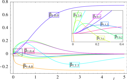
Figure 5: Time evolution of the expansion coefficients $\beta_{1,k,l}(t)$ from Table II for $D=1$, $\gamma=1$, $\mu=0$ and $\sigma=0.5$.

V VARIATIONAL PERTURBATION THEORY

In this section we follow Refs. Putz ; Dreger and perform a variational resummation of the cumulant expansion in close analogy to Section III.2. By doing so, we variationally calculate the probability density $\mathcal{P}(x,t)$ for an arbitrarily large coupling constant $g$ with $\gamma>0$ (anharmonic oscillator) and $\gamma<0$ (double well). In both cases, we obtain probability densities, which originally peaked at the origin, turn into their respective stationary solutions in the long-time limit.

V.1 Resummation Procedure

We aim at approximating the nonlinear drift coefficient (3) by the linear one $-\kappa x$ of a trial Brownian motion with a damping coefficient $\kappa$ which we regard as our variational parameter. To this end we add $-\kappa x$ to the nonlinear drift coefficient (3) and subtract it again:

$$K(x)=-\kappa x-gx^{3}-\left(\gamma-\kappa\right)x\,.$$ (82)

By doing so, we consider the linear term $-\kappa x$ as the unperturbed system and treat all remaining terms in (82) as a perturbation. Such a formal perturbation expansion is performed by introducing an artificial parameter $\delta$ which is later on fixed by the condition $\delta=1$:

$$K(x)=-\kappa x-\delta\left[gx^{3}+\left(\gamma-\kappa\right)x\right]\,.$$ (83)

Performing the rescaling

$$x\to\frac{\tilde{x}}{\beta(\delta)}\,,\hskip 17.07182ptt\to\frac{\tilde{t}}{\beta^{2}(\delta)}\,,\hskip 17.07182ptg\to\frac{\beta^{4}(\delta)\tilde{g}}{\delta}\,$$ (84)

with the scaling factor (33), the FP equation (1) with the drift coefficient (83) is transformed to the original one (22). Due to dimensional reasons also the parameter $\mu,\sigma$ of the initial distribution (58) have to be rescaled according to

$$\mu\to\frac{\tilde{\mu}}{\beta(\delta)}\,,\hskip 17.07182pt\sigma\to\frac{\tilde{\sigma}}{\beta(\delta)}\,.$$ (85)

The rescaling (84), (85) is applied to the cumulant expansion (75), (76). After expanding in powers of $\delta$ and truncating at order $N$, we finally set $\delta=1$ and obtain some $N$th order approximant $p^{(N)}(x,t;\kappa)$ for the cumulant.

Equivalently, the same result follows also from the weak-coupling expansion of the cumulant (75), (76):

$$p^{(N)}(x,t)=\ln\mathcal{P}_{\gamma}(x,t)+\sum_{n=1}^{N}p_{n}(x,t)g^{n}\,.$$ (86)

Treating in (82) the linear drift coefficient $-\kappa x$ as the unperturbed term and all remaining terms as a perturbation corresponds then to the substitution (39) with the abbreviation (40). Thus inserting (39) in (86), a reexpansion in powers of $g$ up to the order $N$ together with the resubstitution (40) leads also to $p^{(N)}(x,t;\kappa)$ Putz .

If we could have performed this procedure up to infinite order, the variational parameter $\kappa$ would have dropped out of the expression, as the original stochastic model (3) does not depend on $\kappa$. However, as our calculation is limited to a finite order $N$, we obtain an artificial dependence on $\kappa$, i.e. some $N$th order approximant $p^{(N)}(x,t;\kappa)$, which has to be minimized according to the principle of minimal sensitivity Stevenson . Thus we search for local extrema of $p^{(N)}(x,t;\kappa)$ with respect to $\kappa$, i.e. from the condition

$$\left.\frac{\partial p^{(N)}(x,t;\kappa)}{\partial\kappa}\right|_{\kappa=\kappa^{(N)}_{\rm opt}(x,t)}=0\,.$$ (87)

It may happen that this equation is not solvable within a certain region of the parameters $x,t$. In this case we look for zeros of higher derivatives instead in accordance with the principle of minimal sensitivity Stevenson , i.e. we determine the variational parameter $\kappa$ from solving

$$\left.\frac{\partial^{m}p^{(N)}(x,t;\kappa)}{\partial\kappa^{m}}\right|_{\kappa=\kappa^{(N)}_{\rm opt,m}(x,t)}=0\,.$$ (88)

The solution $\kappa^{(N)}_{\rm opt}(x,t)$ from (87) or (88) yields the variational result

$$P(x,t)\approx\frac{\exp\left[p^{(N)}\left(x,t;\kappa^{(N)}_{\rm opt}(x,t)\right)\right]}{\displaystyle\int_{-\infty}^{+\infty}\exp\left[p^{(N)}\left(x^{\prime},t;\kappa^{(N)}_{\rm opt}(x^{\prime},t)\right)\right]dx^{\prime}}$$ (89)

for the probability density. Note that variational perturbation theory does not preserve the normalization of the probability density. Although the perturbative result is still normalized in the usual sense to the respective perturbative order in the coupling constant $g$, this normalization is spoilt by choosing an $x$-dependent damping constant $\kappa^{(N)}_{\rm opt}(x,t)$. Thus we have to normalize the variational probability density according to (89) at the end Putz (compare the similar situation for the variational ground-state wave function in Refs. Florian ; Kunihiro ).

V.2 Anharmonic Oscillator $(\gamma>0)$

The variational procedure described in the last section is now applied for determining the time evolution of the probability density in case of the nonlinear drift coefficient (3) with $\gamma>0$. By doing so, the optimization of the variational parameter $\kappa$ is performed for each value of the variable $x$ at each time $t$. The result of such a calculation with the parameters $g=D=1$, $\gamma=\sigma=0.1$ and $\mu=0$ is shown in Figure 6 for the time interval $0\leq t\leq 20$. Figure 6 (a) depicts the optimal variational parameter $\kappa$ which is the largest solution from (87). For small times, the optimal variational parameter reveals a $x^{2}$-dependence. For large values of $t$, the variational parameter becomes independent of $x$ which corresponds to the expectation that the probability density converges towards the stationary one. In Figure 6 (b) the respective variational results for the distribution are compared with the cumulant expansion. The latter shows insofar a wrong behavior as it has two maxima whereas the numerical solution has only one. The variationally determined probability density is depicted by dots which correspond to the optimal variational parameters in Figure 6 (a). We observe on this scale nearly no deviation between the variational and the numerical distribution, thus already the first-order variational results are quite satisfactory.

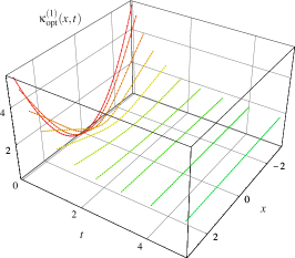
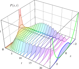
 (a)  (b) (c)

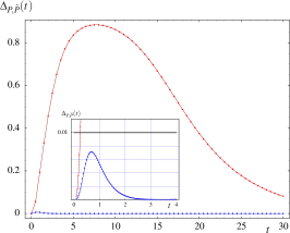
Figure 6: Time evolution of probability density from variational optimization for $g=D=1$, $\gamma=\sigma=0.1$, and $\mu=0$. (a) Largest variational parameter $\kappa$ determined from (87), colors code different times corresponding to the distributions shown in (b). (b) Dots correspond to variational parameters of (a) and coincide on this scale with numerical solutions of FP equation as represented by the lines through the dots. Cumulant expansions are shown as gray areas. At the front the stationary distribution $\mathcal{P}_{\text{stat}}(x)$ and the corresponding potential $\Phi(x)$ are depicted. (c) Distance (90) between variational and cumulant expansion from numerical solution of FP equation.

In order to quantify the quality of our approximation, we introduce the distance between two distributions $\mathcal{P}(x,t)$ and $\tilde{\mathcal{P}}(x,t)$ at time $t$ according to

$$\Delta_{\mathcal{P},\tilde{\mathcal{P}}}(t)=\frac{1}{2}\int_{-\infty}^{+\infty}\left|\mathcal{P}(x,t)-\tilde{\mathcal{P}}(x,t)\right|dx\,.$$ (90)

If both distributions are normalized and positive, the maximum value for the distance $\Delta_{\mathcal{P},\tilde{\mathcal{P}}}(t)$ is $1$ and corresponds to the case that the distributions have no overlap. However, if they coincide for all $x$, the distance $\Delta_{\mathcal{P},\tilde{\mathcal{P}}}(t)$ vanishes. Thus small values of $\Delta_{\mathcal{P},\tilde{\mathcal{P}}}(t)$ indicate that both distributions are nearly identical. In Figure 6 (c) we compare the time evolution of the distance (90) between the variational distribution and the cumulant expansion from the numerical solution of the corresponding FP equation, respectively. We observe that the variational optimization leads for all times to better results than the cumulant expansion, both being indistinguishable for very small and large times, as expected.

V.3 Double Well $(\gamma<0)$

Now we discuss the more complicated problem of a nonlinear drift coefficient (3) with $\gamma<0$. The corresponding potential (21) has the form of a double well, i.e. it decreases harmonically for small $x$ and becomes positive again for large $x$, so that a stationary solution exists (see the front of Figure 7(b)). Strictly speaking, the cumulant expansion developed in Section IV.5 makes no sense for $\gamma<0$ as the unperturbed system $g=0$ does not have a normalizable solution. This problem is reflected in the time evolution of the cumulant expansion coefficients $\beta_{n,k,l}(t)$ which are listed in Table 2 and depicted in Figure 8 for the order $n=1$. In contrast to the case $\gamma>0$ in (81), the coefficient $\beta_{1,4,0}(t)$ vanishes for $\gamma<0$ so that the cumulant expansion (75)–(77) does not even lead to the correct stationary solution (23), (26) up to first order in $g$. In the limit $t\to\infty$ the only nonvanishing expansion coefficients $\beta_{1,k,l}(t)$ read

$$\gamma>0: \lim_{t\to\infty}\beta_{1,0,2}(t)=\frac{3D^{2}(D-2\gamma\sigma^{2})}{2\gamma(D-\gamma\sigma^{2})}\,,\hskip 5.69054pt\lim_{t\to\infty}\beta_{1,2,0}(t)=\frac{3}{2\gamma}\,,$$ (91)

$$\lim_{t\to\infty}\beta_{1,0,4}(t)=\frac{D^{3}}{4(D-\gamma\sigma^{2})^{4}}\,.$$

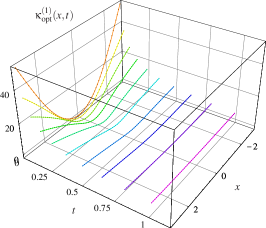
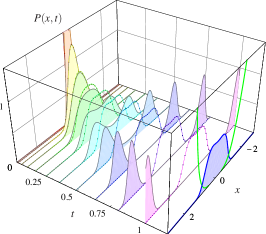
 (a)  (b) (c)

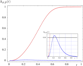
Figure 7: Time evolution of probability density from variational optimization for $g=10$, $D=1$, $\gamma=-1$, $\sigma=0.1$ and $\mu=0$. (a) Largest variational parameter $\kappa$ determined from (87), colors code different times corresponding to the distributions shown in (b). (b) Dots correspond to variational parameters of (a) and coincide on this scale with numerical solutions of FP equation as represented by the lines through the dots. Cumulant expansions are shown as gray areas. At the front the stationary distribution $\mathcal{P}_{\text{stat}}(x)$ and the corresponding potential $\Phi(x)$ are depicted. (c) Distance (90) between variational and cumulant expansion from numerical solution of FP equation.

The results of the first-order variational calculation of the probability density are summarized in Figure 7 for the parameters $g=10$, $D=1$, $\gamma=-1$, $\sigma=0.1$, and $\mu=0$. Due to the strong nonlinearity, we could determine the optimal variational parameter $\kappa$ from solving (87) for all $x$ and $t$ as shown in Figure 7 (a). As expected the cumulant expansion diverges for larger times $t$ as illustrated in Figure 7 (b). Despite of this the variational distribution lies precisely on top of the numerical solutions of the FP equation. This impressive result is also documented in Figure 7(c) where the cumulant expansion shows for increasing time $t$ no overlap with the numerical solution, whereas the distance between the variational and the numerical distribution decreases.

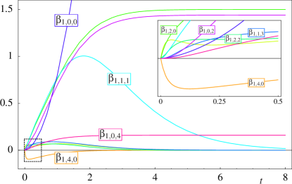
Figure 8: Time evolution of the expansion coefficients $\beta_{1,k,l}(t)$ from Table II for $D=1$, $\gamma=-1$, $\mu=0$, and $\sigma=0.5$.

Even more difficult is the case of a weak nonlinearity where the two minima of the double well are more pronounced. Therefore, the variational calculation has also been performed for the parameter values $g=0.1$, $D=1$, $\gamma=-1$, $\sigma=0.1$, and $\mu=0$. For small times one obtains again a continuous optimal variational parameter $\kappa^{(1)}_{\rm opt}(x,t)$ from solving (87) for all $x$. However, there exists a critical time $t_{\rm crit}\approx 1.6$ beyond which condition (87) has different solution branches depending on $x$. In general such a critical point exists, if the equations:

$$\left[\begin{pmatrix}1\\ \partial/\partial\kappa\\ \partial/\partial x\end{pmatrix}\frac{\partial p^{(N)}(x,t;\kappa)}{\partial\kappa}\right]_{\{x=x_{\rm crit},t=t_{\rm crit},\kappa=\kappa^{(N)}_{\rm crit}\}}=\begin{pmatrix}0\\ 0\\ 0\end{pmatrix}$$ (92)

have a solution $\{x_{\rm crit},t_{\rm crit},\kappa_{\rm crit}\}$. For the case at hand we find $x_{\rm crit}=\pm 2.267$, $t_{\rm crit}=1.618$ and $\kappa_{\rm crit}=-1.326$. The corresponding surface of zeros and the critical points are depicted in Figure 9.

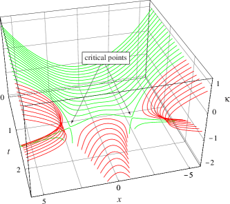
Figure 9: Zeros of $\partial p^{(1)}(x,t;\kappa)/\partial\kappa$ with continuous solutions for $t<t_{\rm crit}=1.618$ and disconnected branches beyond.

As it remains unclear how these branches should be combined for evaluating the probability density, we resort to zeros of higher derivatives (88) that are continuous for all times. For small values of $t$ we find one, two and three continuous zeros for the first, second and third derivative, respectively, as shown in Figure 10 for $t=1.2$. The smallest zero of the second and third derivative reach a critical point at $t_{\rm crit}=1.5284$ and $t_{\rm crit}=1.4588$. The larger zeros have continuous solutions for all values of $t$, as shown in Figure 11 for $t=1.7$.

Figure 12 shows the distance between variational and cumulant expansion from numerical solution of FP equation for these different branches of zeros. Apparently there is no easy choice of the right branch of zeros, which gives good results at all times. While $\kappa_{\rm opt,3b}$ gives good results at small times, it fails to approach the stationary solution. The largest zero $\kappa_{\rm opt,3c}$ of the third derivative on the other hand is unusable for small $t$, but gives good results for later times.

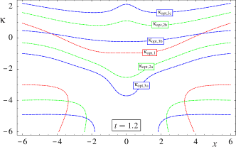
Figure 10: Zeros of (88) for $m=\{1,2,3\}$ at $t=1.2$, before reaching any critical time.

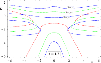
Figure 11: Zeros of (88) for $m=\{1,2,3\}$ at $t=1.7$. The smallest branch of zeros for each derivative has reached a critical point and dissected in disconnected branches.

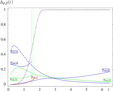
Figure 12: Distance (90) between variational and cumulant expansion from numerical solution of FP equation for different branches of zeros. The smallest zero of each derivative reaches a critical time at $t\approx 1.6$.

Assuming we had no knowledge of the numerical solution, we need to find a way to switch the solution branch from $\kappa_{\rm opt,3b}$ to $\kappa_{\rm opt,3c}$. In order to determine a suitable time to change the branch of zeros from $\kappa_{\rm opt}(x,t)$ to $\kappa^{\prime}_{\rm opt}(x,t)$, we consider the deviation of the moments of the corresponding distributions

$$\Delta^{n}_{\kappa_{\rm opt},\kappa^{\prime}_{\rm opt}}(t)=\frac{\int_{-\infty}^{+\infty}\left|x^{n}\left[P(x,t;\kappa_{\rm opt})-P(x,t;\kappa^{\prime}_{\rm opt})\right]\right|dx}{\int_{-\infty}^{+\infty}\left|x^{n}P_{\rm stat}(x,t)\right|dx}\,.$$ (93)

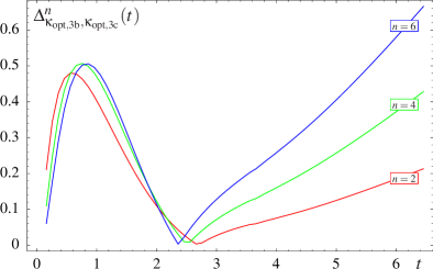
Figure 13: Distance (93) between moments of distributions determined from variationally from different branches of zeros of the third derivative.

Figure 13 shows the distance (93) for the branches of zeros $\kappa_{\rm opt,3b}(x,t)$ and $\kappa_{\rm opt,3c}(x,t)$ for the first three even moments $n={2,4,6}$. We find, that the distributions are in good agreement at $t\approx 2.6$, so we choose to combine the solution for $\kappa_{\rm opt,3b}(x,t)$ for $t<2.6$ with the solution for $\kappa_{\rm opt,3c}(x,t)$ for $t>2.6$. The combined result is shown in Figure 14. The distance (90) between variational expansion and numerical solution of the FP equation for this case exhibits a small kink at $t\approx 2.6$ due to the change in the branch of zeros. Furthermore, in comparison with the other cases in Figures 6 and 7 this distance is relatively large which underlines that this is, indeed, a difficult variational problem. Note, however, that the combined solution succeeds in approaching the stationary solution for large times.

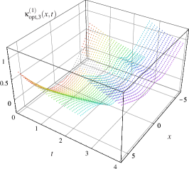
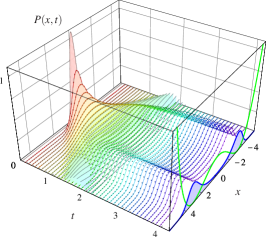
 (a)  (b) (c)

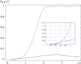
Figure 14: Time evolution of probability density from variational optimization for $g=0.1$, $D=1$, $\gamma=-1$, $\sigma=0.1$, and $\mu=0$. (a) Variational parameter $\kappa$ determined from (88) for $m=3$, colors code different times corresponding to the distributions shown in (b). For $t<2.6$ we selected the branch of zeros $\kappa_{\rm opt,3b}$, whereas for $t>2.6$ the branch $\kappa_{\rm opt,3c}$ was used. Outlined dots are interpolated zeros (see text). (b) Dots correspond to variational parameters of (a) and coincide on this scale with numerical solutions of FP equation as represented by the lines through the dots. Cumulant expansions are shown as gray areas. At the front the stationary distribution $\mathcal{P}_{\text{stat}}(x)$ and the corresponding potential $\Phi(x)$ are depicted. (c) Distance (90) between variational and cumulant expansion from numerical solution of FP equation.

We remark that the variational approach of Ref. Okopinska is related to ours. In contrast to our method, one obtains there in case of the difficult double well problem $g=0.1$, $\kappa=-1$ a unique solution of the extremal condition (87) for all $x$ and $t$. However, the resulting probability density shows for larger times $t$ significant deviations from our, and from numerical solutions of the FP equation.

V.4 Higher Orders

High-order variational calculations have been performed for the double well with the parameters $g=10$, $D=1$, $\gamma=-1$ in case of an initially Gaussian-distributed probability density peaked at the origin, i.e. $\sigma=0.1,\mu=0$ for $t=0.23$. This time was chosen due to its large distance between the variational result and the numerical solution in order to reduce possible errors in the numerical solution. The order of magnitude of the systematic error of the numerical solution can be estimated by comparing the numerical solution of the harmonic problem, e.g. $g=0$, with the exact solution that is available for that case. We find that the error of the numerical solution is about $10^{-6}$, which is smaller that the pointsize used in Figure 15. The first three variational orders, shown in Figure 15, converge exponentially to the numerical solution of the FP equation.

Figure 15: Distance (90) between numerical solution of FP equation and the first three variational calculations for $g=10$, $\gamma=-1$, $D=1$, $\sigma=0.1$, $\mu=0$ and $t=0.23$.

VI SUMMARY

We have presented high-order variational calculations for the probability density $\mathcal{P}(x,t)$ of a stochastic model with additive noise which is characterized by the nonlinear drift coefficient (3). A comparison with numerical results shows an exponential convergence of our variational resummation method with respect to the order. We hope that VPT will turn out to be useful also for other applications in Markov theory as, for instance, the calculation of Kramer rates Haenggi1 (see the recent variational calculation tunneling amplitudes from weak-coupling expansions in Ref. HampKleinert1 ), the treatment of stochastic resonance Haenggi2 , or the investigation of Brownian motors Reimann .