Monte Carlo simulations of bosonic reaction-diffusion systems

Abstract

An efficient Monte Carlo simulation method for bosonic reaction-diffusion systems which are mainly used in the renormalization group (RG) study is proposed. Using this method, one-dimensional bosonic single species annihilation model is studied and, in turn, the results are compared with RG calculations. The numerical data are consistent with RG predictions. As a second application, a bosonic variant of the pair contact process with diffusion (PCPD) is simulated and shown to share the critical behavior with the PCPD. The invariance under the Galilean transformation of this boson model is also checked and discussion about the invariance in conjunction with other models are in order.

I Introduction

The reaction-diffusion (RD) systems have become a paradigm for studying certain physical, chemical, and biological systems P97 . In the study of the RD systems on a lattice via Monte Carlo (MC) simulations, particles involved in the dynamics usually have hard core exclusion property. In other words, MC simulations have been interested in the lattice systems where multiple occupancy at a lattice point is prohibited. These particles are often referred to as fermions, but this paper prefers the term “hard core particles.” Meantime, the renormalization-group (RG) calculations that have been applied successfully to several RD systems are in many cases based on the path integral formalism for classical particles without hard core exclusion, or, if we are allowed to abuse terminology, bosons bosonF ; Lee94 ; CT96 . On this account, the comparison of the numerical studies to the RG calculations is sometimes nontrivial.

There are two ways to fill a gap between numerical and analytical studies. One is to make a path integral formula for hard core particles which is suitable for the RG calculations. Actually, this path has been sought and some formalisms are suggested PKP00 ; vW01 ; PjP05 . The other is to find a numerical method to simulate boson systems. In this context, numerical integration studies of the equivalent Langevin equations to boson systems have been performed BAF97 ; CD99 ; PL99 ; DCM04 . However, it is not always possible to find an equivalent Langevin equation G83 . By the same token, the applicability of this approach is somewhat restricted. Thus, another numerical method is called for. To our knowledge, no algorithm to simulate general bosonic RD systems directly has been suggested and to find such a algorithm is still a challenging topic.

This paper suggests an algorithm to simulate the bosonic RD systems. Section II is devoted to a heuristic explanation of the algorithm to simulate general bosonic single species RD systems. In Sec. III, the numerical method applies to some bosonic RD systems. At first, the single species annihilation models with various conditions are simulated, along with the comparison to the RG predictions. Then, a bosonic version of the pair contact process with diffusion is discussed, focusing on the universality and Galilean invariance. Section IV summarizes the works.

II Algorithm

This section explains the algorithm suitable for MC simulations of bosonic RD systems. Although the discussion in this section is restricted to single species cases, the extension to multispecies problems is straightforward.

The reaction dynamics of diffusing bosons is represented as

$$nA\stackrel{{\scriptstyle\lambda_{nm}}}{{\longrightarrow}}(n+m)A,$$ (1)

where $n\geq 0$, $m\geq-n$, $m\neq 0$, and $\lambda_{nm}$ is the transition rate. Each particle diffuses with rate $D$ on a $d$ dimensional hypercubic lattice. The periodic-boundary conditions are assumed, but other boundary conditions do not limit the validity of the algorithm. Configurations are specified by the occupation number $\rho_{\bm{x}}$ ($\geq 0$) at each lattice point ${\bm{x}}$. A configuration is denoted as $\{\rho\}$ which means $\{\rho_{{\bm{x}}}|{\bm{x}}\in\bm{L}^{d}\}$, where $\bm{L}^{d}$ stands for the set of the lattice points and the cardinality of $\bm{L}^{d}$ is $L^{d}$. The master equation which describes stochastic processes modeled by Eq. (1) takes the form G83 ; K97

$$\frac{\partial P}{\partial t}=D\sum_{\langle{\bm{x}},{\bm{y}}\rangle}\left((\rho_{\bm{x}}+1)\hat{E}_{{\bm{x}},{\bm{y}}}-\rho_{\bm{x}}\right)P$$ (2)

$$+\sum_{n,m}\lambda_{nm}\sum_{{\bm{x}}}\left(f(\rho_{\bm{x}}-m,n)\hat{C}_{{\bm{x}},m}-f(\rho_{\bm{x}},n)\right)P,$$

where $P=P(\{\rho\},t)$ is the probability with which the configuration of the system is $\{\rho\}$ at time $t$, $\langle{\bm{x}},{\bm{y}}\rangle$ means the nearest-neighbor pair (${\bm{x}},{\bm{y}}\in\bm{L}^{d}$), $f(\rho_{\bm{x}},n)=(\rho_{\bm{x}}!)/(\rho_{\bm{x}}-n)!$ is the number of ordered $n$ tuples at site ${\bm{x}}$ of the configuration $\{\rho\}$, and $\hat{E}_{{\bm{x}},{\bm{y}}}$ and $\hat{C}_{{\bm{x}},m}$ are operators affecting $P(\{\rho\},t)$ such that

$$\hat{E}_{{\bm{x}},{\bm{y}}}P =P(\{\cdots,\rho_{\bm{x}}+1,\rho_{\bm{y}}-1,\cdots\};t),$$ (3)

$$\hat{C}_{{\bm{x}},m}P =P(\{\cdots,\rho_{\bm{x}}-m,\cdots\};t).$$

The master equation implies that during infinitesimal time interval $dt$, the average number of transition events for the configuration $\{\rho\}$ is

$$E(dt, \{\rho\})=dt\sum_{{\bm{x}},n}\left(2dD\delta_{n,1}+\sum_{m}\lambda_{nm}\right)f(\rho_{\bm{x}},n)$$ (4)

$$=dt\sum_{{\bm{x}},n}\left(2dD\delta_{n,1}+\sum_{m}n!\lambda_{nm}\right)g(\rho_{\bm{x}},n),$$

where $g(\rho_{\bm{x}},n)=f(\rho_{\bm{x}},n)/n!=\binom{\rho_{\bm{x}}}{n}$ is the number of (nonordered) $n$ tuples at site ${\bm{x}}$. Therefore, the first step for MC simulations is to select one of $n$ tuples with an equal probability. For the convenience of description and better understanding, we introduce a model dependent function $h(\rho_{\bm{x}},n)=\epsilon_{n}g(\rho_{\bm{x}},n)$, where $\epsilon_{n}$ takes 1 (0) if $D\delta_{n,1}+\sum_{m}\lambda_{nm}$ is nonzero (zero). The meaning of $\epsilon_{n}$ is straightforward; we do not have to consider the reaction dynamics with transition rate zero (see below).

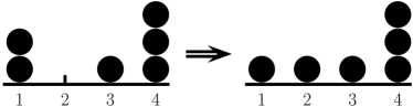
Figure 1: An example of a configuration change of a one-dimensional RD system with $L=4$ due to hopping. The black circle signifies a particle and numbers below the horizontal line indicate the lattice point. A particle at site 1 hops to site 2.

The simplest way to implement the selection is as follows: First a site ${\bm{x}}$ is selected with probability $N_{\bm{x}}/M$, where $N_{\bm{x}}={\sum_{n}}h(\rho_{\bm{x}},n)$ which will be called the number of accessible states at site ${\bm{x}}$ and $M=\sum_{\bm{x}}N_{\bm{x}}$. Then, $n$ is chosen with probability $h(\rho_{\bm{x}},n)/N_{\bm{x}}$ which is zero if $\epsilon_{n}=0$. For this procedure, the array of the number of particles at all sites, say ${\bm{\rho}}[~{}]$ (${\bm{\rho}}[{\bm{x}}]=\rho_{\bm{x}}$), is necessary.

However, it is not efficient because there are too many floating number calculations. For a faster performance, we introduce two more arrays, say list[ ] and act[ ][ ]. The array list[ ] refers the location of any $n$ tuple. Each element of list[ ] takes the form $({\bm{x}},\ell)$, where ${\bm{x}}$ is a site index and $\ell$ lies between 1 and $N_{\bm{x}}$ ($1\leq\ell\leq N_{\bm{x}}$). From $\ell$ and ${\bm{\rho}}[{\bm{x}}]$, which $n$ tuple is referred by the array list[ ] is determined. If $\ell\leq h(\rho_{\bm{x}},0)$, $n=0$ is implied. Else if $\ell\leq h(\rho_{\bm{x}},0)+h(\rho_{\bm{x}},1)$, $n=1$ is meant. Else if $\ell\leq h(\rho_{\bm{x}},0)+h(\rho_{\bm{x}},1)+h(\rho_{\bm{x}},2)$, $\ell$ indicates one of pairs at site ${\bm{x}}$, and so on. In case the total number of accessible states in the system is $M$, the size of list[ ] is $M$ and all elements of list[ ] should satisfy that ${\tt list}[p]\neq{\tt list}[q]$ if $p\neq q$ ($1\leq p,q\leq M$). Hence, the random selection of an integer between 1 and $M$ is equivalent to the choice of one $n$ tuple among $M$ accessible states with an equal probability. The array act[ ][ ] is the inverse of the list[ ], that is, ${\tt list}[s]=({\bm{x}},\ell)$ corresponds to ${\tt act}[{\bm{x}}][\ell]=s$.

Table 1: An example of making two arrays referring each other from the configuration shown in Fig. 1. Two columns on the left (right) hand side correspond to the configuration before (after) the hopping event.

Before		After
list[1]=(1,1)	act[1][1]=1	list[1]=(1,1)	act[1][1]=1
list[2]=(1,2)	act[1][2]=2	list[2]=(4,6)	act[2][1]=9
list[3]=(1,3)	act[1][3]=3	list[3]=(4,5)	act[3][1]=4
list[4]=(3,1)	act[3][1]=4	list[4]=(3,1)	act[4][1]=5
list[5]=(4,1)	act[4][1]=5	list[5]=(4,1)	act[4][2]=6
list[6]=(4,2)	act[4][2]=6	list[6]=(4,2)	act[4][3]=7
list[7]=(4,3)	act[4][3]=7	list[7]=(4,3)	act[4][4]=8
list[8]=(4,4)	act[4][4]=8	list[8]=(4,4)	act[4][5]=3
list[9]=(4,5)	act[4][5]=9	list[9]=(2,1)	act[4][6]=2
list[10]=(4,6)	act[4][6]=10

After selecting ${\bm{x}}$ and $n$, the transition $nA\rightarrow(n+m)A$ occurs with the probability of $n!\lambda_{nm}\Delta t$ for all possible $m$, where $\Delta t$ is independent from configurations. Provided $n=1$ is selected, in addition to reaction processes, a particle at ${\bm{x}}$ hops to one of the nearest neighbors with probability $D\Delta t$. To make the transition probability have a meaning, $\Delta t$ should satisfy

$$\left(2dD\delta_{n,1}+\sum_{m}n!\lambda_{nm}\right)\Delta t\leq 1,$$ (5)

for all $n$. Time is increased by $\Delta t/M$. On average, this algorithm generates $E(\Delta t,\{\rho\})$ transition events during time interval $\Delta t$. After the system’s evolving, three arrays, ${\bm{\rho}}$, list, and act, are updated in a suitable way (see below).

Through an example, how the system evolves in silico is to be clarified. Consider a RD system with $\epsilon_{n}=0$ for $n\geq 3\text{ and }n=0$. In this case, $N_{\bm{x}}=\sum_{n}h(\rho_{x},n)=g(\rho_{\bm{x}},1)+g(\rho_{\bm{x}},2)=\rho_{\bm{x}}(\rho_{\bm{x}}+1)/2$ will be used. Assume that we are given a configuration ${\bm{\rho}}[1]=2$, ${\bm{\rho}}[2]=0$, ${\bm{\rho}}[3]=1$, and ${\bm{\rho}}[4]=3$ ($N_{1}=3$, $N_{2}=0$, $N_{3}=1$, $N_{4}=6$, hence $M=10$); see Fig. 1. Complete lists of two arrays list[ ] and act[ ][ ] for this configuration are illustrated on the left-hand side of Table 1. The algorithm starts from selecting one number between 1 and $M$, randomly. Let us assume that 2 is selected, which makes ${\tt list}[2]$ to be checked. Since ${\tt list}[2]=(1,2)$ and $2\leq{\bm{\rho}}[1]$, a particle dynamics at site 1 will be attempted. Again assume that a hopping to the site 2 whose probability is $D\Delta t$ occurs, which results in a change of the configuration as shown in Fig. 1. Accordingly, three arrays should be updated. Figure 2 shows how the evolution is coded (based on the language c). In this code, rho[$x$] is the number of particles at site $x$ ($=\rho_{x}$), N[$x$] is the number of accessible states at site $x$ ($=N_{x}$), and each element of list[ ] is treated as an array. The first (second) for loop signifies the decreasing (increasing) of the number of accessible states at site 1 (2), which can be used for any particle number decreasing (increasing) events. The code generates the lists on the right-hand side of Table 1. Time is increased by $\Delta t/10$. Then again choose one number between 1 to 9, randomly, and so on.

Figure 2: A program which updates three arrays ${\bm{\rho}}[~{}]$, ${\tt list}[~{}]$, and ${\tt act}[~{}][~{}]$ after the hopping event shown in Fig. 1.

Equipped with the numerical methods, Sec. III studies some bosonic RD systems which show scaling behavior.

III Applications

III.1 Single species annihilation model

The algorithm explained in the previous section is applied to a one-dimensional single species annihilation model which corresponds to $\lambda_{nm}=0$ unless $n=2$ and $m=-2$. For saving the writing effort, let us rename $\lambda_{2,-2}\mapsto\lambda$. The renormalization-group calculation predicts that the annihilation fixed point corresponds to $\lambda=\infty$ Lee94 . Infinite pair annihilation rate means that two particles occupying the same site by any chance will be removed instantaneously. Accordingly, at most one particle can reside at each site. Hence, the boson model with infinite annihilation rate is equivalent to the diffusion-limited annihilation model (DLAn) of hard core particles which can be solved exactly S00 . It is known that the particle density of the DLAn starting from the random initial condition decays as

$$\rho(t)=\lim_{L\rightarrow\infty}\frac{1}{L}\sum_{x=1}^{L}\rho_{x}(t)=\frac{1}{\sqrt{8\pi Dt}}(1+O(1/t)).$$ (6)

This behavior does not depend on the initial density. Since renormalized coupling constant flows to the annihilation fixed point, the asymptotic behavior of the density for finite $\lambda$ is expected to be the same as Eq. (6). Besides, it is expected that the smaller the value of $\lambda$, the later the system enters the scaling regime. Actually, these predictions are tested for the annihilation model of hard core particles PPK01 . However, to our knowledge, there is no satisfactory numerical test for the RG predictions using a boson model comment .

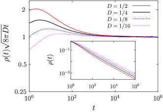
Figure 3: (Color online) A log-log plot of $\rho(t)\sqrt{8\pi Dt}$ as a function of $t$ for various $D$ with $\lambda=\frac{1}{2}$ and $\rho_{0}=1$. All curves approach to 1 as $t$ increases. Inset: same, but density is not multiplied by $\sqrt{8\pi Dt}$.

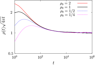
Figure 4: (Color online) A log-log plot of $\rho(t)\sqrt{4\pi t}$ vs $t$ for various $\rho_{0}$ with $D=\frac{1}{2}$ and $\lambda=\frac{1}{2}$. In the asymptotic regime, all data sets show the same behavior.

The Poisson distribution is used as an initial condition, which can be implemented if we randomly distributed $\rho_{0}L$ particles on the lattice. For this distribution, the probability that $q$ particles reside at site ${\bm{x}}$ is

$$P_{x}(q)=\left(\begin{array}[]{c}\rho_{0}L\\ q\end{array}\right)\left(\frac{1}{L}\right)^{q}\left(1-\frac{1}{L}\right)^{\rho_{0}L-q}\sim\frac{\rho_{0}^{q}}{q!}e^{-\rho_{0}},$$ (7)

where $L$ is assumed to be sufficiently large and $q\ll\rho_{0}L$. Using the algorithm explained in the previous section and varying $D$, $\lambda$, and $\rho_{0}$, we simulated the one-dimensional annihilation model. The system size is $2^{16}$ and the number of independent samples is 200 for each data set.

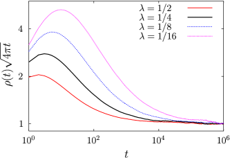
Figure 5: (Color online) A log-log plot of $\rho(t)\sqrt{4\pi t}$ vs $t$ for various $\lambda$ with $D=\frac{1}{2}$ and $\rho_{0}=1$. Although the system with smaller $\lambda$ enters the scaling regime slowly, all curves eventually meet for large $t$.

Figure 3 shows the decaying behavior of the density for $D=\frac{1}{2}$, $\frac{1}{4}$, $\frac{1}{8}$, and $\frac{1}{16}$ with $\rho_{0}=1$ and $\lambda=\frac{1}{2}$. Each curves approaches to $1/\sqrt{8\pi Dt}$ as the RG calculation predicted. We also check the initial condition dependence, by simulating systems with various initial density 2, 1, $\frac{1}{2}$, and $\frac{1}{4}$ with $D=\frac{1}{2}$ and $\lambda=\frac{1}{2}$. Figure 4 shows the initial condition independence of the asymptotic behavior. Finally, we also confirm that the asymptotic behavior is not affected by $\lambda$, see Fig. 5. As expected, the system with smaller $\lambda$ enters the scaling regime later. The MC simulation for bosonic annihilation models confirms the predictions of the RG study Lee94 .

III.2 Pair contact process with diffusion

The pair contact process with diffusion (PCPD) is a RD system of diffusing hard core particles with two competing dynamics of $2A\rightarrow 3A$ (fission) and $2A\rightarrow 0$ (annihilation), which shows a continuous transition HH04 . At first sight, the bosonic variant of the PCPD might be regarded as the boson model with $\lambda_{nm}=0$ except $\lambda_{21}$ and $\lambda_{2,-2}$. However, this variant does not show a continuous transition and there is no steady state in its active (fission dominating) phase HT97 . To have a well-defined steady state in all phases, a mechanism to keep the density from blowing up is required. Introducing a triple reaction such as $3A\rightarrow 2A$, one can get a model with well-defined steady states. Although the boson model with $\lambda_{nm}=0$ except $\lambda_{21}$, $\lambda_{2,-2}$, and $\lambda_{3,-1}$ has been expected to show a continuous transition HH04 , MC simulation results for this type of boson model which will be called “BPCPD” has yet been reported in the literature, although a parallel update bosonic model with so-called soft-constraint was studied KC03 .

Using parameter values $D=\frac{1}{2}$, $\lambda_{3,-1}=\frac{1}{6}$, $\lambda_{2,-2}=p/2$, and $\lambda_{21}=(1-p)/2$ where $p$ is the tuning parameter, the critical behavior of the BPCPD is studied. As an initial condition, we set $\rho_{\bm{x}}=2$ for all ${\bm{x}}$ ($1\leq{\bm{x}}\leq L$). Figure 6 shows the decaying behavior at criticality of two order parameters, the particle and pair densities which are defined as

$$\rho_{1}(t) =\frac{1}{L}\sum_{\bm{x}}\langle\rho_{\bm{x}}\rangle_{t},$$ (8)

$$\rho_{2}(t) =\frac{1}{L}\sum_{\bm{x}}\langle\rho_{\bm{x}}(\rho_{\bm{x}}-1)\rangle_{t},$$

where $\langle\cdots\rangle_{t}$ means the average over ensembles at time $t$. The system size in use is $2^{15}$ and all samples (around $10^{3}$ samples are independently simulated) up to observation time ($\sim 2.5\times 10^{6}$ MC steps) have at least one site with two or more particles. The critical point is found to be $p_{c}=0.148~{}79(1)$ with the critical exponent $\beta/\nu_{\|}=0.205(5)$ which is estimated from the effective exponent

$$-\delta(t)=\frac{\ln[\rho_{1,2}(t)]-\ln[\rho_{1,2}(t/m)]}{\ln m},$$ (9)

with $m=10$. At criticality, $\delta(t)$ approaches to $\beta/\nu_{\|}$ as $t$ goes to infinity. The simulation results are consistent with the previous works within error bars KC03 ; PhP05a . Hence, we conclude that the BPCPD has the same critical scaling with the PCPD.

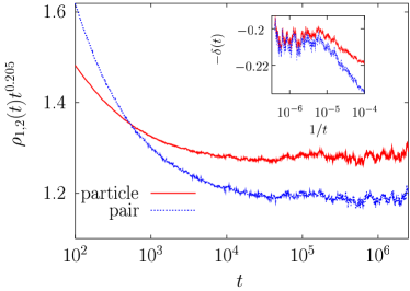
Figure 6: (Color online) Time dependence of the particle and pair densities multiplied by $t^{\beta/\nu_{\|}}$ with $\beta/\nu_{\|}=0.205$ in semilogarithmic plot at criticality for the BPCPD. Inset: effective exponents of the order parameters at $p=0.148~{}79$.

Following the path integral formalism for bosonic RD systems bosonF , the action of the BPCPD, $S=\int dt~{}d{\bm{x}}{\cal L}$, after taking the (naive) space-time continuum limit has the form

$${\cal L}=\bar{\phi}(\partial_{t}-D\nabla^{2})\phi+g_{1}\bar{\phi}\phi^{2}+\lambda_{3}\bar{\phi}\phi^{3}+g_{2}\bar{\phi}^{2}\phi^{2}+\cdots,$$ (10)

which is the same as one studied in Ref. JWDT04 which is derived from path integral formalism for the exclusive particle systems introduced in Ref. vW01 . It is argued, however, via RG calculations JWDT04 and numerical studies PhP05a ; PhP05b that Eq. (10) is inappropriate for studying the critical behavior of the PCPD using the RG techniques. Nonetheless, we will show that the Galilean invariance (GI) of the BPCPD, which is anticipated from Eq. (10), is still correct in the strong sense (see below).

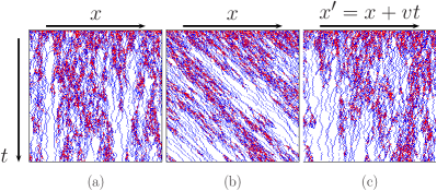
Figure 7: (Color online) Space-time configuration for the unbiased and biased BPCPD models at criticality. Blue (red) dots represent the sites with only one particle (at least two particles) and white dots stand for the empty sites. (a) and (b) are configurations of the BPCPD with $D_{R}=\frac{1}{2}$ and $D_{R}=1$, respectively. (c) is the same as (b) except that the space coordinate is Galilean transformed with $v=D_{R}-D_{L}=1$.

For some RD systems, biased diffusion only changes nonuniversal constants such as the critical point and does not affect the critical behavior. Examples are the driven branching annihilating random walks (DBAW) studied in Ref. PhP05a . Such systems will be called to have the GI in the weak sense (GIweak). Why the critical point is dependent on the bias strength is understandable within the framework of Ref. PjP05 . Using the path integral formalism for hard core particles introduced in Ref. PjP05 , the terms appearing in the action due to the bias with the strength $v$ take the form

$${\cal L}_{\textrm{bias}}=v\left(\bar{\phi}_{\bm{x}}\partial_{\|}\phi_{\bm{x}}-\bar{\phi}_{\bm{x}}^{2}\phi_{\bm{x}}\partial_{\|}\phi_{\bm{x}}\right),$$ (11)

where $\partial_{\|}$ is the lattice gradient defined as $\partial_{\|}\phi_{\bm{x}}\equiv(\phi_{{\bm{x}}+\bm{e}_{\|}}-\phi_{{\bm{x}}-\bm{e}_{\|}})/2$ with $\bm{e}_{\|}$ the unit vector along the bias direction. The derivation of Eq. (11) is shown in the Appendix. The Galilean transformation gauges away the first term in Eq. (11), but cannot remove the second term. Since the second term in Eq. (11) is irrelevant in the RG sense for the DBAW, this does not affect the universal behavior, but the very existence of this irrelevant term can change the critical point. Therefore, the DBAW is of the GIweak. Meanwhile, the PCPD is not of the GI even in the weak sense PhP05a . Since it is shown that the field theory with the action (10) is not viable JWDT04 , we cannot extract any information from Eq. (11) concerning the driven pair contact process with diffusion (DPCPD). To understand the DPCPD and the PCPD from the field theoretical point of view, more elaborated studies are required.

The bias diffusion of bosons does not generate the second term in Eq. (11). In this context, the Galilean transformation totally gets rid of the effect of bias for bosons. Hence, two systems with or without bias have the same probability distribution, let alone the critical behavior. These systems will be called to have the GI in the strong sense (GIstrong). Consider a one-dimensional bosonic RD system with reaction dynamics in Eq. (1) in which each particle hops to the right (left) with rate $D_{R}$ ($D_{L}$). The GIstrong for this model means that whatever value $D_{R}$ takes with the constraint $D_{R}+D_{L}=2D$ (constant), the system shares the probability distribution with the unbiased model ($D_{R}=D_{L}=D$). It is checked numerically for various $D_{R}$ with $D_{R}+D_{L}=1$, whether the BPCPD has the GIstrong or not. We observed that the particle and pair densities have the same behavior at the same $p$ within statistical error (not shown here). In Fig. 7, space-time configurations of the BPCPD models with the unbiased diffusion ($D_{R}=D=\frac{1}{2}$), fully biased diffusion ($D_{R}=2D=1$), and the Galilean transformation for the full bias case are shown. After Galilean transformation, no noticeable difference between biased and unbiased cases is observed. For comparison, we present in Fig. 8 the space-time configuration of the PCPD and the DPCPD studied in Ref. PhP05a . As the Galilean transformed space-time configuration shows, the bias cannot be removed in the DPCPD. The Galilean transformation generates the biased motion of the paired particles which shows the existence of the relative bias between isolated particles and paired ones. Although the validity of Eq. (10) as an appropriate action for the RG study regarding the PCPD is rather problematic, any single species bosonic RD systems with on-site reactions are conjectured to have the GIstrong.

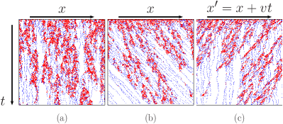
Figure 8: (Color online) Space-time configuration for (a) the PCPD and (b) the DPCPD at criticality studied in Ref. PhP05a . Blue (red) dots represent the isolated particles (particles which are members of pairs) and white dots stand for the empty sites. (c) is the same as (b) except that the space coordinate is Galilean transformed with $v=1$.

The discussion about the GIstrong should be restricted to boson models with random sequential update dynamics. If the dynamics occurs in a parallel way as in Ref. KC03 , the GI argument from the invariance of the local action like Eq. (10) under the Galilean transformation is not directly applicable. Even worse, the one dimensional system with $p_{R}=1$ (for the definition of $p_{R}$, see the next paragraph) is reduced to a single-site problem which is not expected to show phase transition. Notwithstanding, except this pathological case, the soft-constraint PCPD (SCPCPD) studied in Ref. KC03 is expected to have the GIweak KCcomment .

To understand what is happening in the SCPCPD, let us explain the dynamics of the model. During unit time, changes of a configuration occur in two steps. At first, every particle hops to the right (left) with probability $p_{R}$ ($p_{L}$) and stays still with probability $p_{S}$ ($p_{R}+p_{L}+p_{S}=1$). In Ref. KC03 , $p_{R}=p_{L}=\frac{1}{2}$ and $p_{S}=0$ are used. After the hopping events, reactions occur at all sites. Rather interestingly, the model with $p_{L}=0$ is statistically equivalent to the system with $p_{S}=0$ provided $p_{R}$ is the same. When $p_{S}=0$, particles at the even sites do not interact with those in the odd sites. For example, see Fig. 1 and regard the left figure of it as a configuration for the SCPCPD with $p_{S}=0$ under the condition of the periodic boundary. At the end of the hopping event, particles at sites 1 and 3 (2 and 4) move on to sites 2 and 4 (1 and 3). Thus, a system with size $2L$ (let us call it system $A$) can be considered two independent systems with size $L$ (call it system $B$), if we interpret the hopping events to the left in the system $A$ as a staying event in the system $B$. Since the system with $p_{L}=0$ has a bias effect in diffusion except the pathological case of $p_{R}=1$, the GI for the SCPCPD is in a sense predictable.

As a final remark, we would like to mention how the DPCPD behavior can be observed in the BPCPD model. As explained before, the bias applied to all particles has no effect. As was done for the SCPCPD in Ref. PhP05a , if different bias is applied to a particle at singly occupied sites and a particle at multiply occupied sites, the DPCPD behavior such as mean-field-like exponents, logarithmic corrections, etc., was observed (not shown here). This unusual bias cannot be included in the action like Eq. (10) in a simple way, so this DPCPD behavior is not contradictory to the GIstrong of the BPCPD.

IV Summary

To summarize, an efficient algorithm is proposed to simulate the general bosonic reaction-diffusion systems and applies to the single species annihilation model and the bosonic variant of the pair contact process with diffusion. For the single species annihilation model, renormalization group predictions are confirmed numerically. The BPCPD model is found to belong to the PCPD universality class and maintains the Galilean invariance in the strong sense. Due to the lack of the analytical predictions for the PCPD, only the comparison of our results to published simulation results are possible.

*

Appendix A Derivation of Eq. (11)

From the path integral formalism for RD systems of hard core particles introduced in Ref. PjP05 , Eq. (11) will be derived in this appendix. Since the master equation is linear and the formalism in PjP05 does not mix different dynamics, it is enough to consider the diffusion of hard core particles. For more detailed accounts, see Ref. PjP05 .

In general, the master equation becomes the imaginary time Schrödinger equation with (in general non-Hermitian) Hamiltonian $\hat{H}$ such that

$$\frac{\partial}{\partial t}|P;t\rangle=-\hat{H}|P;t\rangle,$$ (12)

where $|P;t\rangle=\sum_{\{\rho\}}P(\{\rho\},t)|\{\rho\}\rangle$ and $|\{\rho\}\rangle=\prod_{\bm{x}}|\rho_{x}\rangle$ with $\rho_{x}$ taking either 1 (occupied) or 0 (vacant). To write down the Hamiltonian, introduced are the creation and annihilation operators for hard core particles in single species models which satisfy the following commutation relations:

$$\{\hat{a}_{\bm{x}}^{\dagger},\hat{a}_{\bm{x}}\} =1,\quad\{\hat{a}_{\bm{x}},\hat{a}_{\bm{x}}\}=\{\hat{a}_{\bm{x}}^{\dagger},\hat{a}_{\bm{x}}^{\dagger}\}=0,$$ (13)

$$[\hat{a}_{\bm{x}},\hat{a}_{{\bm{x}}^{\prime}}] =[\hat{a}_{\bm{x}}^{\dagger},\hat{a}_{{\bm{x}}^{\prime}}^{\dagger}]=0.$$

Actually, these operators are nothing but the Pauli matrices. Using creation and annihilation operators, terms appearing in the Hamiltonian due to diffusion of hard core particles in the single species RD systems can be written as $\hat{H}_{D}=\sum_{\bm{x}}\hat{H}_{\bm{x}}$ with

$$\hat{H}_{\bm{x}}= \sum_{i=1}^{d}\Bigl{[}\left(D+\delta_{i,\|}\frac{v}{2}\right)(\hat{n}_{\bm{x}}\hat{v}_{{\bm{x}}+{\bm{e}}_{i}}-\hat{a}_{\bm{x}}\hat{a}_{{\bm{x}}+{\bm{e}}_{i}}^{\dagger})$$ (14)

$$+\left(D-\delta_{i,\|}\frac{v}{2}\right)(\hat{n}_{\bm{x}}\hat{v}_{{\bm{x}}-{\bm{e}}_{i}}-\hat{a}_{\bm{x}}\hat{a}_{{\bm{x}}-{\bm{e}}_{i}}^{\dagger})\Bigr{]},$$

where $\hat{n}_{\bm{x}}=\hat{a}_{\bm{x}}^{\dagger}\hat{a}_{\bm{x}}$ is the number operator, $\hat{v}_{\bm{x}}=1-\hat{n}_{\bm{x}}$, ${\bm{e}}_{i}$ is the unit vector along $i$ direction, and hopping is biased along the $\|$ direction.

The differential equation of the generating function $F$ which is defined as

$$F(\{\bar{\varphi}\};t)\equiv\sum_{\{\rho\}}\left(\prod_{\bm{x}}{\bar{\varphi}_{\bm{x}}}^{\rho_{\bm{x}}}\right)P(\{\rho\};t)=\langle\{\bar{\varphi}\}|P;t\rangle,$$ (15)

where

$$\langle\{\bar{\varphi}\}|\equiv\prod_{\bm{x}}\left(\langle 0|_{\bm{x}}+\bar{\varphi}\langle 1|_{\bm{x}}\right),$$ (16)

takes the form

$$\frac{\partial}{\partial t}F=-\langle\{\bar{\varphi}\}|\hat{H}|P;t\rangle.$$ (17)

The generating function (15) corresponds to Eq. (15) of Ref. PjP05 with the prescription (18a) in Ref. PjP05 . Since

$$\langle\{\bar{\varphi}\}|\hat{a}_{\bm{x}}^{\dagger} = \bar{\varphi}_{\bm{x}}(1-\bar{\varphi}_{\bm{x}}\hat{\varphi}_{\bm{x}})\langle\{\bar{\varphi}\}|,$$ (18)

$$\langle\{\bar{\varphi}\}|\hat{a}_{\bm{x}} = \hat{\varphi}_{\bm{x}}\langle\{\bar{\varphi}\}|,$$ (19)

$$\langle\{\bar{\varphi}\}|\hat{n}_{\bm{x}} = \bar{\varphi}_{\bm{x}}\hat{\varphi}_{\bm{x}}\langle\{\bar{\varphi}\}|,$$ (20)

$$\langle\{\bar{\varphi}\}|\hat{v}_{\bm{x}} = (1-\bar{\varphi}_{\bm{x}}\hat{\varphi}_{\bm{x}})\langle\{\bar{\varphi}\}|,$$ (21)

where $\hat{\varphi}_{\bm{x}}=\partial/\partial\bar{\varphi}_{\bm{x}}$, one can find the partial differential equations for the generating function such that

$$\frac{\partial}{\partial t}F=-\hat{\cal L}(\{\bar{\varphi}\},\{\hat{\varphi}\})F,$$ (22)

with normal ordered evolution operator $\hat{\cal L}$ which reads

$$\hat{\cal L}(\{\bar{\varphi}\},\{\hat{\varphi}\})=\sum_{\bm{x}}\Bigg{\{}v\left[\bar{\varphi}_{\bm{x}}\partial_{\|}\bar{\varphi}_{\bm{x}}-\bar{\varphi}_{\bm{x}}^{2}\hat{\varphi}_{\bm{x}}\partial_{\|}\hat{\varphi}_{\bm{x}}\right]$$ (23)

$$+D\left[-\bar{\varphi}_{\bm{x}}\nabla_{\bm{x}}^{2}\hat{\varphi}_{x}+\sum_{i}(\bar{\varphi}_{\bm{x}}-\bar{\varphi}_{{\bm{x}}+{\bm{e}}_{i}})^{2}\hat{\varphi}_{\bm{x}}\hat{\varphi}_{{\bm{x}}+{\bm{e}}_{i}}\right]\Bigg{\}}$$

$$+(\textrm{terms due to reactions}),$$

where $\nabla^{2}_{\bm{x}}$ is the lattice Laplacian defined as $\nabla^{2}_{\bm{x}}f({\bm{x}})=\sum_{i=1}^{d}(f({\bm{x}}+{\bm{e}}_{i})+f({\bm{x}}-{\bm{e}}_{i})-2f({\bm{x}}))$, and $\partial_{\|}$ is the lattice gradient along the $\|$ direction defined as $\partial_{\|}f({\bm{x}})=(f({\bm{x}}+{\bm{e}}_{\|})-f({\bm{x}}-{\bm{e}}_{\|}))/2$. Since Eq. (22) is a linear equation, we can write down the path integral solution with the action PjP05

$$S=\int dt\left[\bar{\phi}\partial_{t}\phi+{\cal L}(\{\bar{\phi}\},\{\phi\})\right],$$ (24)

which completes the derivation of Eq. (11).

References

- (1) See, for example, Nonequilibrium Statistical Mechanics in One Dimension, edited by V. Privman (Cambridge University Press, Cambridge, UK, 1997).
- (2) M. Doi, J. Phys. A 9, 1465 (1976); 9, 1479 (1976); P. Grassberger and M. Scheunert, Fortschr. Phys. 28, 547 (1980); L. Peliti, J. Phys. (Paris) 46, 1469 (1985).
- (3) B. P. Lee, J. Phys. A 27, 2633 (1994).
- (4) J. Cardy and U. C. Täuber, Phys. Rev. Lett. 77, 4780 (1996).
- (5) S.-C. Park, D. Kim, and J.-M. Park, Phys. Rev. E 62, 7642 (2000).
- (6) F. van Wijland, Phys. Rev. E 63, 022101 (2001).
- (7) S.-C. Park and J.-M Park, Phys. Rev. E 71, 026113 (2005).
- (8) M. Beccaria, B. Allés, and F. Farchioni, Phys. Rev. E 55, 3870 (1997).
- (9) W. J. Chung and M. W. Deem, Physica A 265, 486 (1999).
- (10) L. Pechenik and H. Levine, Phys. Rev. E 59, 3893 (1999).
- (11) I. Dornic, H. Chaté, and M. A. Muñoz, Phys. Rev. Lett. 94, 100601 (2005).
- (12) C. W. Gardiner, Handbook of Stochastic Methods for Physics, Chemistry, and the Natural Sciences (Springer-Verlag, Berlin, 1983).
- (13) N.G. van Kampen, Stochastic Processes in Physics and Chemistry, enlarged edition (Elsevier, Amsterdam, 1997).
- (14) See, e.g., G.M. Schütz, in Phase Transitions and Critical Phenomena, edited by C. Domb and J. L. Lebowitz (Academic Press, London, 2000), Vol. 19 and references therein.
- (15) See, e.g., S.-C. Park, J.-M. Park, and D. Kim, Phys. Rev. E 63, 057102 (2001).
- (16) There is a numerical integration study of the equivalent (complex) Langevin equation in Ref. BAF97 , but the results only confirm the decay exponent.
- (17) For a review, see M. Henkel and H. Hinrichsen, J. Phys. A 37, R117 (2004).
- (18) M. J. Howard and U. C. Täuber, J. Phy. A 30, 7721 (1997).
- (19) J. Kockelkoren and H. Chaté, Phys. Rev. Lett. 90, 125701 (2003).
- (20) S.-C. Park and H. Park, Phys. Rev. Lett. 94, 065701 (2005).
- (21) H.-K. Janssen, F. van Wijland, O. Deloubriére, and U. C. Täuber, Phys. Rev. E 70, 056114 (2004).
- (22) S.-C. Park and H. Park, Phys. Rev. E 71, 016137 (2005).
- (23) The observation of the GI for the SCPCPD in Ref. PhP05a should be understood in the weak sense.