Synchronization in complex networks with age ordering

Abstract

The propensity for synchronization is studied in a complex network of asymmetrically coupled units, where the asymmetry in a given link is determined by the relative age of the involved nodes. In growing scale-free networks synchronization is enhanced when couplings from older to younger nodes are dominant. We describe the requirements for such an effect in a more general context and compare with the situations in non growing random networks with and without a degree ordering.

From the brain over the Internet to human society, complex networks are the prominent candidates to describe sophisticated collaborative dynamics in many areas revmod . Complex networks are collections of dynamical nodes connected by a wiring of edges exhibiting complex topological properties. Of particular interest are the so called small-world (SW) and scale free (SF) wirings. SW are intermediate wirings between regular lattices (RL) and random networks (RN) watts98 . They are characterized by a path-length $\ell$ between any two nodes much shorter than a RL, but yet a clustering structure much higher than a RN. The basic property of SW is the logarithmic scaling of $\ell$ with the network size $N$ ($\ell\propto\log N$), in contrast to the linear scaling of RL. A specific example of SW is the SF configuration, in which the degree $k$ (the number of edges in a node) follows a power law distribution $p(k)\sim k^{-\gamma}$. A SF network can be grown by adding successively new nodes to the network and connecting them with the already existing ones by a preferential attachment rule barabasi99 . SW and SF properties were found in many networks in nature, such as the World Wide Web, the internet connection wiring, power grids and transportation networks, neural networks, metabolic and protein networks.

Recently, the dynamics of complex networks has been extensively investigated with regard to collective (synchronized) behaviors booksPhaseSynchr , with special emphasis on the interplay between complexity in the overall topology and local dynamical properties of the coupled units complNetSync ; barahona02 ; lai03 . Most of the previous works assumed the local units to be symmetrically connected with uniform undirected coupling strengths (unweighted links). This simplification, however, does not match satisfactorily the peculiarities of many real networks. In ecological systems, for instance, the non uniform weight in prey-predator interactions plays a crucial role in determining the food web dynamics maccan98 . Similarly, the interaction between individuals in social networks social is never symmetric, rather it depends upon several social factors, such as age, social class or influence, personal leadership or charisma.

In this Letter, we analyze networks of asymmetrically coupled dynamical units. By explicitly relating the asymmetry in the connections to an age order among different nodes, we will give evidence that age ordered networks provide a better propensity for synchronization (PFS). In particular we will show that the three main ingredient maximizing PFS are i) heterogeneity in the network topology allowing for the existence of nodes with very large degrees (hubs) together with nodes with very small degrees (non hubs), ii) asymmetry in the connections forcing a preferential coupling direction from hubs to non hubs, and iii) a structure of connected hubs in the network.

We here adopt the idea that the direction of an edge can be determined by an age ordering between the connected nodes. For growing networks (such as SF) the age order is naturally related to the appearance order of the node during the growing process. We consider a network of $N$ linearly coupled identical systems. The equation of motion reads

$$\begin{array}[]{l l}\dot{\bf x}_{i}={\bf F}({\bf x}_{i})-\sigma\sum_{j=1}^{N}G_{ij}{\bf H}[{\bf x}_{j}],&i=1,\ldots,N,\end{array}$$ (1)

where $\dot{\bf x}={\bf F}({\bf x})$ governs the local dynamics of the vector field ${\bf x}_{i}$ in each node, ${\bf H}[{\bf x}]$ is a linear vectorial function, and $\sigma$ is the coupling strength. $G_{ij}$ is a zero row-sum coupling matrix with off diagonal entries $G_{ij}=-{\cal A}_{ij}\frac{\Theta_{ij}}{\sum_{j\in K_{i}}\Theta_{ij}}$, where ${\cal A}$ is the adjacency matrix, and $\Theta_{ij}=\frac{1-\theta}{2}$ $\left(\Theta_{ij}=\frac{1+\theta}{2}\right)$ for $i>j$ ($i<j$). $K_{i}$ is the set of $k_{i}$ neighbors of the $i^{\text{th}}$ node, and the parameter $-1<\theta<1$ governs the coupling asymmetry in the network. Precisely, $\theta=0$ yields a symmetric coupling, while the limit $\theta\to-1$ ($\theta\to+1$) gives a unidirectional coupling where the old (young) nodes drive the young (old) ones. Asymmetric coupling was recently also established for non identical space extended fields prljean , where asymmetry consisted in forcing preferentially the dynamical regime of a field into the other.

The network PFS can be inspected by linear stability of the synchronous state (${\bf x}_{i}={\bf x}_{s},\forall i$). By diagonalizing the variational equation, one obtains $N$ blocks of the form $\dot{\zeta}_{i}=\text{J}{\bf F}({\bf x}_{s})\zeta_{i}+\sigma\lambda_{i}{\bf H}[\zeta_{i}]$, that only differ by the eigenvalues of the coupling matrix $\lambda_{i}$ (here J is the Jacobian operator). The behavior of the largest Lyapunov exponent associated with $\nu=\sigma\lambda_{i}$ (also called master stability function pecora98 ) fully accounts for the linear stability of the synchronization manifold. Namely, the synchronous state (associated to $\lambda_{1}=0$), is stable if all the remaining blocks, associated to $\lambda_{i}$ ($i\geq 2$), have negative Lyapunov exponents.

For a generic $\theta$, our coupling matrix is asymmetric, and therefore its spectrum is contained in the complex plane ($\lambda_{1}=0;\ \lambda_{l}=\lambda^{r}_{l}+j\lambda^{i}_{l},\ l=2,\ldots,N$). Moreover, since all elements of $G$ are real, non real eigenvalues appear in pairs of complex conjugates. In the following we will order the eigenvalues of $G$ for increasing real parts. Gerschgorin’s circle theorem gershgorin asserts that $G$’s spectrum is fully contained within the union of circles ($C_{i}$) having as centers the diagonal elements of $G$ ($d_{i}$), and as radii the sums of the absolute values of the other elements in the corresponding rows ($\{\lambda_{l}\}\subset\cup_{i}C_{i}\left[d_{i},\sum_{j\neq i}\mid G_{ij}\mid\right]$).

By construction, the diagonal elements of $G$ are normalized to 1 in all possible cases. It is crucial to emphasize the physical and mathematical relevance of this choice. Physically, this normalization prevents the coupling term from being arbitrarily large (or arbitrarily small) for all possible network topologies and sizes, thus making it a meaningful realization of what happens in many real world situations (such as neuronal networks) where the local influence of the environment on the dynamics does not scale with the number of connections. Mathematically, since $G$ is a zero row-sum matrix (and furthermore $d_{i}=\sum_{j\neq i}\mid G_{ij}\mid$ because all non zero off diagonal elements are negative), this warrants in all cases that $G$’s spectrum is fully contained within the unit circle centered at 1 on the real axis ($\mid\lambda_{l}-1\mid\leq 1,\ \forall l$), giving the following inequalities: i) $0<\lambda^{r}_{2}\leq\ldots\leq\lambda^{r}_{N}\leq 2$, and ii) $\mid\lambda^{i}_{l}\mid\leq 1,\ \forall l$. This latter property is essential to provide a consistent and unique mathematical framework within which one can formally assess the relative merit of one topology against another for optimal PFS independent of the network size or the local dynamics.

Figure 1: $\lambda^{r}_{N}$ and $\lambda^{r}_{2}$ (a), $\frac{\lambda^{r}_{N}}{\lambda^{r}_{2}}$(b), and $M$ (c) vs. $\theta$ for SF ($m=5$ and $B=0$, solid lines) and RN (dashed lines). All quantities and all other network parameters are specified in the text.

Let $\cal R$ be the bounded region in the complex plane where the master stability function provides a negative Lyapunov exponent. The stability condition for the synchronous state is that the set $\{\sigma\lambda_{l},l=2,\ldots,N\}$ be entirely contained in $\cal R$ for a given $\sigma$. The best PFS is then assured when both the ratio $\frac{\lambda^{r}_{N}}{\lambda^{r}_{2}}$ and $M\equiv\max_{l}\{\mid\lambda^{i}_{l}\mid\}$ are simultaneously made as small as possible.

With the help of such stipulations, we start with analyzing the effects of heterogeneity in the node degree distribution. This is done by comparing the PFS of a class of SF networks with different degree distributions with a highly homogeneous RN. The used class of SF networks is obtained by a generalization of the preferential attachment growing procedure barabasi99 . Namely, starting from $m+1$ all to all connected nodes, at each step a new node is added with $m$ links, connecting to old nodes with probability $p_{i}=\frac{k_{i}+B}{\sum_{j}(k_{j}+B)}$ ($k_{i}$ being the degree of the $i^{\text{th}}$ node, and $B$ a tunable real parameter, representing the initial attractiveness of each node). The $\gamma$ exponent of the power law scaling in the degree distribution $p(k)\sim k^{-\gamma(B,m)}$ is then given by $\gamma(B,m)=3+\frac{B}{m}$ in the thermodynamic ($N\to\infty$) limit netInNature . While the average degree is by construction $\langle k\rangle=2m$ (thus independent of $B$), the heterogeneity of the degree distribution can be strongly modified by $B$. This induces convergence of higher order moments of $p(k)$, in contrast with the case $B=0$ that recovers the original preferential attachment rule barabasi99 .

For comparison, a highly homogeneous Erdös-Rényi RN erdos is considered, with connection probability $P=\frac{2m}{N-1}$ (giving same average degree $\langle k\rangle=2m$), with an arbitrary initial age ordering. Fig. 1a) shows $\lambda^{r}_{N}$ and $\lambda^{r}_{2}$ vs. $\theta$ for SF with $m=5$ and $B=0$ (solid line) and for the chosen RN (dashed line). All calculations refer to ensemble averages over 24 different realizations of networks with 500 nodes. For RN, the curve $\lambda^{r}_{N}(\theta)$ [$\lambda^{r}_{2}(\theta)$] displays a minimum [a maximum] for $\theta=0$, showing that asymmetry here deteriorates the network PFS. At variance, for SF the difference between $\lambda^{r}_{N}$ and $\lambda^{r}_{2}$ continuously shrinks, as $\theta$ decreases. As a consequence, Fig. 1b) reports the behavior of the eigenratio $\frac{\lambda^{r}_{N}}{\lambda^{r}_{2}}$, making it clear that while the best PFS in RN is obtained for the symmetric case ($\theta=0$), SF shows better (worse) PFS in the asymmetric case for $\theta\to-1$ ($\theta\to 1$). As for the imaginary part of the spectra, Fig. 1c) reports $M$ vs. $\theta$, indicating only very small differences between SF and RN in the whole range of the asymmetry parameter, and highlighting that the contribution to PFS of the imaginary part of the spectra does not depend significantly on the specific network structure. These findings have been consistently observed in subsequent results.

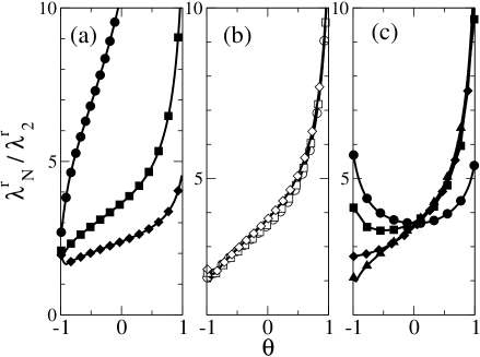
Figure 2: $\frac{\lambda^{r}_{N}}{\lambda^{r}_{2}}$ vs. $\theta$ for (a) SF with $B=0$ and $m=2$ (circles), 5 (squares), 10 (diamonds); (b) SF with $m=5$ and $B=0$ (circles), 5 (squares), and 10 (diamonds); (c) RN with arbitrary age order (circles), RN with age depending on degree (squares), SF with $m=5$ and $B=0$ without connection between nodes 1 and 5 (diamonds), and SF with $m=5$ and $B=0$ (triangles).

The second step of our study is the investigation of PFS in SF at different $m$ and $B$ values. In Fig. 2 (a), PFS is compared for different $m$ for $B=0$. Since $m$ determines the average degree, as $m$ increases, the average connectivity increases and synchronizability is naturally enhanced. The most important point is that the monotonically decreasing behavior of $\frac{\lambda^{r}_{N}}{\lambda^{r}_{2}}$ with $\theta$ persists for all $m$, indicating that synchronization is always enhanced when $\theta$ becomes smaller. In Fig. 2 (b), PFS is compared for $m=5$ and for various values of $B$, altering the exponent of the degree distribution. For all $B$ values, the same enhancement for negative $\theta$ was observed. Therefore, one can conclude that in aged growing networks PFS depends on the average degree, but the asymmetry enhanced synchronization phenomenon does not depend on heterogeneity.

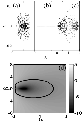
Figure 3: Distribution of $G$’s eigenvalues in the complex plane for SF with $m=2$, $B=0$ and $\theta=-0.8$ (a), $\theta=0$ (b), and $\theta=0.8$ (c). (d) Master stability function in the complex plane for coupled Rössler oscillators.

This leads us to discuss the main point of our study, concerning the determination of the essential topological ingredients enhancing PFS in weighted (aged) networks. The first ingredient is that the weighting must induce a dominant interaction from hub to non hub nodes. This can be easily understood by a simple example: the case of a star network consisting of a single large hub (the center of the star) and several non-hub nodes connected to the hub. When the dominant coupling direction is from the non-hub nodes to the hub node, synchronization is impossible because the hub receives a set of independent inputs from the different non-hub nodes. In the reverse case (when the center drives the periphery of the star) synchronization can be easily achieved. The very same mechanism occurs in our SF case. Indeed, for positive (negative) $\theta$ values, the dominant coupling direction is from younger (older) to older (younger) nodes. Now, in SF the minimal degree of a node is by construction $m$ and older nodes are more likely to display larger degrees than younger ones, so that a negative $\theta$ here induces a dominant coupling direction from hubs to non-hub nodes.

The second ingredient is that the network contains a structure of connected hubs influencing the other nodes. In our SF case, the normalization in the off diagonal elements of $G$ norma assures that hubs receive an input from a connected node scaling with the inverse of their degree, and therefore the structure of hubs is connected always with the rest of the network in a way that is independent on the network size.

In order to make evident the validity of these claims, we have performed a careful analysis on enhanced PFS over a series of ad-hoc modified networks. The results are summarized in Fig. 2 (c). First, we have reordered the node age in RN according to each node degree. The resulting $\frac{\lambda^{r}_{N}}{\lambda^{r}_{2}}(\theta)$ (curve with squares) shows now a minimum for an asymmetric configuration ($\theta\approx-0.5$), in contrast to the case with arbitrary aging (curve with circles). This confirms the need of a dominant interaction from hubs to non hubs for improving PFS, also for highly homogeneous networks. As for the second ingredient, starting from a SF with $m=5$ and $B=0$ (curve with triangles), we artificially disconnected the initially existing link between the first and fifth network nodes. These are indeed the two hubs with highest degree in the SF configuration. The result is shown in the curve with diamonds, where one sees that such a small perturbation (the difference in the two networks is limited to only a link) is already sufficient to substantially weaken the PFS. The situation remains however better than the two RN cases, indicating that the structure of growing aged network inherently enhances synchronization.

Figure 4: $\langle D\rangle$ (see text for definition) vs. $\sigma$ for RN (a) and for SF ($m=2,B=0$, b). In both graphs the curves with circles, squares, diamonds, up triangles, and left triangles refer to $\theta=~{}-0.8,~{}-0.4,~{}0,~{}0.4,~{}0.8$, respectively.

Finally, we prove the validity of our arguments by applying them to networks of coupled chaotic Rössler oscillators roe . The dynamics is ruled by Eq. 1, with ${\bf x}=(x,y,z)$, ${\bf F}({\bf x})=[-y-z,\ x+0.165y,\ 0.2+z(x-10)]$, and ${\bf H}[{\bf x}]=x$. The master stability function is depicted in Fig. 3 (d) in the complex plane $\nu=\alpha+j\beta$. The bold solid line (denoting a zero Lyapunov exponent) is the boundary between stability ($\cal R$) and instability regions for the synchronization manifold. The whole network synchronizes when all the eigenvalues of $G$ (multiplied by $\sigma$) locate inside $\cal R$. Figs. 3 (a,b,c) report the location of the $G$ spectrum for SF for $m=2,B=0,N=500$ and with $\theta=-0.8,\ 0,$ and $0.8$, respectively. While for $\theta=0$ the spectrum is real, comparison of (a) and (c) shows that the spectra at negative $\theta$ values are much less dispersed in the complex plane, thus increasing the range of $\sigma$ values for which synchronization can be achieved in the network.

The appearance of the synchronous state can be monitored by looking at the vanishing of the time average (over a window $T$) synchronization error $\langle D\rangle=\frac{1}{T(N-1)}\sum_{j>1}\int_{t}^{t+T}||\mathbf{x}_{j}-\mathbf{x}_{1}||dt^{\prime}$. In the present case, we adopt as vector norm $||\mathbf{x}||=|x|+|y|+|z|$. Fig. 4 reports $\langle D\rangle$ vs. $\theta$ for RN with arbitrary age (a) and for SF with $m=2,B=0$ (b). The curves with circles, squares, diamonds, up triangles, and left triangles refer to $\theta=~{}-0.8,~{}-0.4,~{}0,~{}0.4,~{}0.8$, respectively. While in the RN case the range for synchronization is substantially independent on $\theta$ [reflecting the behavior of $\frac{\lambda^{r}_{N}}{\lambda^{r}_{2}}$ in the dashed line of Fig. 1 (b)], the case with SF [to be compared with the curve with circles in Fig. 2 (a)] confirms that synchronization is strongly affected by the asymmetry. In particular, negative (positive) values of $\theta$ have the effects of increasing (decreasing) the range of coupling strengths over which synchronization occurs with respect to the symmetric case $\theta=0$.

In conclusion we have demonstrated that PFS is enhanced in aged networks of asymmetrically coupled units. In growing SF such enhancement is particularly evident when the dominant coupling direction is from older to younger nodes. Our study allows to individuate the main network topological ingredients at the basis of synchronization enhancement. A key aspect of social organizations is the dynamics of information exchange. Our approach may provide new insights in the study of collective communication or coordination in distributed social networks, as well as useful hints for understanding the formation of social collective behaviors (leading opinions, rumors, political orientations, dominant tastes, habits, fashion). Work partly supported by MIUR-FIRB project n. RBNE01CW3M-001.

References

- (1) R. Albert and A. L. Barabási, Rev. Mod. Phys. 74, 47 (2002).
- (2) D. J. Watts and S. Strogatz, Nature, 393, 440 (1998).
- (3) A. L. Barabási and R. Albert, Science, 286, 509 (1999).
- (4) S. Boccaletti, J. Kurths, G. Osipov, D.L. Valladares and C.S. Zhou, Phys. Rep. 366, 1 (2002).
- (5) L. F. Lago-Fernández, R. Huerta, F. Corbacho and J. A. Sigüenza, Phys. Rev. Lett. 84, 2758 (2000); H. Hong, M.Y. Choi and B.J. Kim, Phys. Rev. E65, 026139 (2002).
- (6) B. Barahona and L. M. Pecora, Phys. Rev. Lett. 89, 054101 (2002).
- (7) T. Nishikawa, A.E. Motter, Y.-C. Lai and F. C. Hoppensteadt, Phys. Rev. Lett. 91, 014101 (2003).
- (8) E. L. Berlow, Nature 398, 330 (1999).
- (9) S. N. Dorogovtsev and J. F. F. Mendes, Phys. Rev. E 62, 1842 (2000); J.J. Ramasco, S. N. Dorogovtsev and R. Pastor-Satorras, Phys. Rev. E 70, 036106 (2004).
- (10) J. Bragard, S. Boccaletti, and H. Mancini, Phys. Rev. Lett. 91, 064103 (2003); J. Bragard, S. Boccaletti, C. Mendoza, H. G. E. Hentschel, and H. Mancini, Phys. Rev. E 70, 036219 (2004).
- (11) L. M. Pecora and T. L. Carroll, Phys. Rev. Lett. 80, 2109 (1998).
- (12) S. A. Gerschgorin, Bull. Acad. Sci. URSS Leningrad 2, 749 (1931); H.E. Bell, Amer. Math. Monthly 72, 292 (1965).
- (13) S. N. Dorogovtsev and J. F. F. Mendes, Adv. Phys. 51, 1079 (2002).
- (14) P. Erdös and A. Rényi, Publ. Math. (Debrecen) 6, 290 (1959).
- (15) For SF growing networks, the non zero off diagonal elements of the coupling matrix are given by , where stands for and , respectively.
- (16) O.E. Rössler, Phys. Lett. A57, 397 (1976).