Resonant plasmon scattering by discrete breathers in Josephson junction ladders

Abstract

We study the resonant scattering of plasmons (linear waves) by discrete breather excitations in Josephson junction ladders. We predict the existence of Fano resonances, and find them by computing the resonant vanishing of the transmission coefficient. We propose an experimental setup of detecting these resonances, and conduct numerical simulations which demonstrate the possibility to observe Fano resonances in the plasmon scattering by discrete breathers in Josephson junction ladders.

I Introduction

Discrete nonlinear Hamiltonian systems generically allow for spatially localized and time periodic states, discrete breathers (DBs), which exist thanks to the interplay between nonlinearity and discreteness reviews . DBs have been detected and studied experimentally in interacting Josephson junction systems binder00a , coupled nonlinear optical waveguides eisenberg98 , lattice vibrations in crystals swanson99 , antiferromagnetic structures schwarz99 , micromechanical cantilever arrays sato03 , Bose-Einstein condensates loaded on optical lattices BEC , layered high-$T_{c}$ superconductors hightc . DBs are predicted also to exist in the dynamics of dusty plasma crystals plasma .

In the transmission problem of small amplitude waves at frequency $\omega_{q}$ through a DB in the particular case of a one-dimensional lattice, the DB acts as a time periodic scattering potential with frequency $\Omega$. Generally, there is an infinite number of scattering paths in such a case, which may lead to a variety of interference phenomena (see Fig. 1). Indeed, perfect reflection was observed for particular wave numbers tcsasf98 ; kimkim00 ; kimkim01 ; sfaemmvf03 . A detailed analysis of this phenomenon shows sfaemvfmvf02 that it is a Fano resonance fano which is based on the phenomenon of destructive interference.

\psfrag{w}{$\omega_{q}$}\psfrag{w-W}{$\omega_{q}-\Omega$}\psfrag{w-2W}{$\omega_{q}-2\Omega$}\psfrag{w-3W}{$\omega_{q}-3\Omega$}\psfrag{w+W}{$\omega_{q}+\Omega$}\psfrag{w+2W}{$\omega_{q}+2\Omega$}\psfrag{w+3W}{$\omega_{q}+3\Omega$}\includegraphics[width=216.81pt]{fig1.eps}

Figure 1: Schematic representation of dynamically generated paths in the frequency domain by a time periodic scattering potential with a period $2\pi/\Omega$. In general, there is an infinite number of paths which may lead to different interference phenomena.

Systems of coupled Josephson junctions with a ladder geometry allow for the experimental excitation and detection of DBs binder00a . A variety of experimental methods allows for a systematic study of DB properties, which have been successfully combined with theoretical calculations and predictions josephsons ; etjjmabtpo01 ; aemsfmvfyzjbp01 ; aemsfbm03 ; flach99:_rotob_josep ; schuster01:_obser_josep . JJLs are quasi-one-dimensional, and allow for the excitation of travelling linear oscillatory waves (usually referred to as plasma waves or plasmons), which can be scattered by DBs. That makes JJLs suitable for the observation of Fano resonances. In addition, Josephson junction systems are dissipative systems including both damping and the presence of an external homogeneous dc bias.

The aim of this paper is to investigate the possibility for the observation of Fano resonances in plasma wave scattering by DBs in Josephson junction ladders (JJLs). We will also discuss the experimental setup for the possible observation of these resonances. We make use of the underdamped regime of dissipation and exploit previous results on Fano resonances which have been obtained for nondissipative systems.

II Model

JJLs are formed by an array of small Josephson junctions that are arranged along the spars and rungs of a ladder, as shown in Fig. 2.

Figure 2: Schematic view of the Josephson junction ladder. Each cross represents a junction. Arrows denote the dc bias flow.

Junctions are denoted by crosses. Each junction consists of two small weakly coupled superconducting islands. The dynamical state of a junction is described by the phase difference $\phi$ (Josephson phase) of the superconducting order parameters of the two islands. When the phase difference does not vary in time $\phi={\mathrm{c}onst}$, the junction is in the superconducting state. Otherwise, the junction is in a resistive state with a nonzero voltage drop $V\propto\dot{\phi}$ (the dot represents differentiation with respect to time).

By using the resistively shunted junction (RSJ) model and Kirchhoff’s laws, we obtain a set of equations for Josephson junction ladders (JJLs) in the following form josephsons ; etjjmabtpo01 ; aemsfmvfyzjbp01

$$\ddot{\phi}_{n}^{v}+\alpha\dot{\phi}^{v}_{n}+\sin\phi_{n}^{v} = \gamma+\frac{1}{\beta_{L}}(\triangle\phi_{n}^{v}+\nabla\phi_{n-1}^{h}-\nabla\tilde{\phi}_{n-1}^{h})$$

$$\ddot{\phi}_{n}^{h}+\alpha\dot{\phi}_{n}^{h}+\sin\phi_{n}^{h} = -\frac{1}{\eta\beta_{L}}(\nabla\phi_{n}^{v}+\phi_{n}^{h}-\tilde{\phi}_{n}^{h})$$ (1)

$$\ddot{\tilde{\phi}}{}^{h}_{n}+\alpha\dot{\tilde{\phi}}{}^{h}_{n}+\sin\tilde{\phi}_{n}^{h} = \frac{1}{\eta\beta_{L}}(\nabla\phi_{n}^{v}+\phi^{h}_{n}-\tilde{\phi}_{n}^{h})\;,$$

where the notations $\triangle f_{n}\equiv f_{n-1}-2f_{n}+f_{n+1}$ and $\nabla f_{n}\equiv f_{n+1}-f_{n}$ are used. The Josephson phases of vertical, upper and lower horizontal junctions in the $n$th cell are denoted by $\phi_{n}^{v}$, $\tilde{\phi}{}_{n}^{h}$ and $\phi_{n}^{h}$ respectively, $\alpha$ is an effective damping, $\gamma$ is the external dc bias across vertical junctions. The discreteness parameter $\beta_{L}=2\pi I_{c}^{V}L/\Phi_{0}$ characterizes the ratio of geometrical cell inductance $L$ and the Josephson inductance of vertical junctions, and $\eta=I_{c}^{H}/I_{c}^{V}$ is the anisotropy parameter of the Ladder. Here, $I_{c}^{V}$ ($I_{c}^{H}$) is the vertical (horizontal) junction critical current (see Ref. schuster01:_obser_josep for details).

III Small amplitude excitations of the superconducting ground state

First we discuss the spectrum of small amplitude excitations (plasmons) around the superconducting ground state $\phi_{n}^{*v}=\arcsin\gamma$ and $\phi_{n}^{*h}=\tilde{\phi}_{n}^{*h}=0$ by linearizing the system (II)

$$\phi_{n}^{v}=\phi^{*v}_{n}+\varphi_{n}^{v}\;,\;\phi_{n}^{h}=\phi_{n}^{*h}+\varphi_{n}^{h}\;,\;\tilde{\phi}_{n}^{h}=\tilde{\phi}_{n}^{*h}+\tilde{\varphi}_{n}^{h}\;,$$ (2)

where $\varphi_{n}^{v}$, $\varphi_{n}^{h}$ and $\tilde{\varphi}_{n}^{h}$ describe the small amplitude excitations. The presence of dissipation leads to the decay of excitations in time. In experiments, the dissipation $\alpha$ can be rather weak (of the order of 0.01 or even less) and usually it is ignored when discussing the small amplitude excitation spectrum josephsons . Here we provide the correct solution in the presence of damping. We can exclude the dissipative term by the following time-dependent transformation

$$\varphi={\mathrm{e}}^{-\frac{\alpha}{2}t}\psi\;.$$ (3)

According to (3) the obtained plane waves are characterized by an exponential decay in time with a characteristic decay time $\tau=2/\alpha$. By solving the equations for $\psi_{n}\sim e^{i(qn-\omega_{q}t)}$ we obtain three plasmon bands $\omega_{1}(q),\omega_{2}(q),\omega_{3}(q)$ (see Appendix A). One of them $\omega_{1}^{2}(q)=1-\frac{\alpha^{2}}{4}$ is dispersionless (i.e. the frequency does not depend on $q$). It is characterized by all vertical junctions being at rest and in-phase excitations of horizontal junctions in each cell. The two other plasmon bands are characterized by $\omega_{2}^{2}(q)<\omega_{1}^{2}(q)$ and $\omega_{3}^{2}(q)>\omega_{1}^{2}(q)$. Note here, that the band $\omega_{2}^{2}(q)$ possesses a rather weak dispersion and becomes dispersionless for $\gamma=0$. In that limit it also coincides with the first band: $\omega_{2}(q)=\omega_{1}(q)$ for $\gamma=0$. Therefore, in the Hamiltonian limit $\alpha=0$ and $\gamma=0$ there is only one plasmon band $\omega_{3}^{2}(q)$ with nonzero dispersion.

IV Discrete breathers

JJLs support dynamic localized states - discrete breathers. A breather is characterized by a few junctions being in the resistive state $\langle\dot{\phi}\rangle\neq 0$ while the others reside in the superconducting state $\langle\dot{\phi}\rangle=0$. The frequency of a DB is proportional to the average voltage drop across the resistive junctions $\Omega_{b}\propto\langle\dot{\phi}\rangle$ and generally depends on the parameters of the system. Different types of DBs have been observed experimentally and numerically josephsons . In the following we focus on DB solutions, which are schematically represented in Fig. 3.

Figure 3: Schematic representations of A- and B- type breather resistive cores in JJLs with one vertical resistive junction. Black spots mark the junctions being in the resistive state while all others are in the superconducting one.

By tuning the external dc bias $\gamma$, a DB state generally follows adiabatically and change its characteristics including voltage drop (frequency), spatial extent etc. We coin such a state a nonresonant DB. This is correct unless the DB solution starts to resonate with the plasmon modes of the unexcited part of the ladder. Such resonances may either lead to a loss of the DB solution, or to the appearance of resonant DBs etjjmabtpo01 ; aemsfmvfyzjbp01 ; schuster01:_obser_josep . These states are characterized by a strong coupling of the DB and the extended plasmon modes of the ladder, and a corresponding voltage locking. Consequently resonant DBs are characterized by their voltage drop (frequency) being nearly independent of the applied external dc bias. Note that resonant DB states do not persist in the dissipationless Hamiltonian limit easily, since the absence of dissipation causes a radiation of the DB energy into the rest of the ladder due to the assumed resonance with the extended ladder modes. In the dissipative case, extended modes are damped, and energy is fed into the system through the breather core, providing with an intricate balance. However DBs with nondecaying tails in Hamiltonian systems might well correspond to resonant DBs in dissipative systems.

V Dissipationless limit and correspondence idea

Let us study the Hamiltonian limit, by neglecting both the dissipation $\alpha$ and the dc bias $\gamma$. In that case we can later apply a well developed numerical scheme for wave scattering. While the wave scattering can be also analyzed for the dissipative case, we use the advantages of DB properties in Hamiltonian systems. In this limit nonresonant DBs become one-parameter families of periodic orbits in phase space. Their general form is

$$\vec{\phi}_{n}(t)=\vec{\kappa}_{n}\Omega_{b}t+\vec{g}_{n}(t)\;,$$ (4)

where the notation $\vec{f}_{n}=\{f_{n}^{v},f_{n}^{h},\tilde{f}^{h}_{n}\}$ for the function of cell $n$ is used. The $j$th component of $\vec{\kappa}_{n}$ is an integer winding number. It is nonzero for a few junctions in the DB’s core and zero for all others. E.g. for the breathers from Fig. 3 we have $\kappa=1$ for all resistive junctions of the A-breather and zero otherwise, while for the B-breather $\kappa=1$ for the resistive horizontal junctions and $\kappa=2$ for the vertical resistive junction. $\vec{g}_{n}(t)$ are periodic functions of time $\vec{g}_{n}(t~{}+~{}\frac{2\pi}{\Omega_{b}})=\vec{g}_{n}(t)$ with exponential decay of amplitudes along the ladder $\max\limits_{t}|g^{j}_{|n|\rightarrow\infty}(t)|~{}\rightarrow~{}0$. The frequency $\Omega_{b}$ is a parameter which changes along the family of solutions.

In the presence of weak dissipation $\alpha$ and dc bias $\gamma$ a given solution from a nonresonant DB family is selected to become an attractor and only slightly changed in its temporal evolution. These changes are small if $\alpha\ll 1$ which we assume. By tuning the external dc bias $\gamma$ we simply scan dissipative nonresonant DBs which are close to their nonresonant DBs of the Hamiltonian limit. For this purpose one can use the relation between $\Omega_{b}$, $\alpha$ and $\gamma$, which is given in Ref. aemsfmvfyzjbp01 . This correspondence idea will be exploited in what follows below.

VI Scattering of waves by discrete breathers: dissipationless case

DBs are dynamic localized excitations. For propagating waves DBs act as time-periodic scattering potentials. Based on results for Hamiltonian lattices tcsasf98 ; kimkim00 ; kimkim01 ; sfaemmvf03 , we expect that such interesting phenomena as resonant transmission and resonant reflection could be observed in JJLs too. Here we focus on the resonant reflection, or Fano resonance. We start with the Hamiltonian limit, where we can rely on recent results on Fano resonances induced by time periodic scattering potentials sfaemvfmvf02 . We predict the position of the resonance and then confirm the prediction using numerical simulations. The extrapolation of the obtained resonances to the non-Hamiltonian case in the presence of non zero damping and bias will be shown to be successfull.

In order to study the scattering problem in the Hamiltonian limit $\alpha=0$ and $\gamma=0$, we linearize the set of equations (II) around a DB (4) by substituting $\vec{\phi}_{n}=\hat{\vec{\phi}}_{n}+\vec{\varphi}_{n}$ with small amplitude excitations $\vec{\varphi}_{n}$

$$\ddot{\varphi}_{n}^{v}+\cos(\hat{\phi}^{v}_{n})\varphi_{n}^{v} = \frac{1}{\beta_{L}}(\triangle\varphi_{n}^{v}+\nabla\varphi_{n-1}^{h}-\nabla\tilde{\varphi}_{n-1}^{h})$$

$$\ddot{\varphi}_{n}^{h}+\cos(\hat{\phi}_{n}^{h})\varphi_{n}^{h} = -\frac{1}{\eta\beta_{L}}(\nabla\varphi_{n}^{v}+\varphi_{n}^{h}-\tilde{\varphi}_{n}^{h})$$ (5)

$$\ddot{\tilde{\varphi}}{}_{n}^{h}+\cos(\hat{\tilde{\phi}}{}_{n}^{h})\tilde{\varphi}^{h}_{n} = \frac{1}{\eta\beta_{L}}(\nabla\varphi_{n}^{v}+\varphi_{n}^{h}-\tilde{\varphi}_{n}^{h})\;.$$

This is a set of linear equations with time-periodic coefficients with the period $T_{b}=\frac{2\pi}{\Omega_{b}}$.

The set of equations (VI) describes scattering of waves by a time-periodic scattering potential. We may estimate the time-averaged scattering potential by replacing $\cos(\hat{\phi})=0$ for a resistive junction and $\cos(\hat{\phi})=1$ for a superconducting junction. The interaction part (right hand side of Eq.(VI)) is not changed. Due to the finite maximum strength of the scattering potential, the expected nonresonant scattering impact can be expected to be weak in general, especially if the plasmon band width (and thus the corresponding group velocity of waves) is large enough. That promises ideal grounds for observing resonant reflection on the background of nearly perfect transmission.

The wave scattering by DBs is studied by using proper boundary conditions, which implies a scattering setup - at the left hand side there are incoming and reflected waves and at the right hand side there are only transmitted ones

$$\vec{\varphi}_{n}(t)=\left\{\begin{array}[]{ll}\vec{I}{\mathrm{e}}^{-{\mathrm{i}}(\omega_{3}(q)t-qn)}+\vec{R}{\mathrm{e}}^{-{\mathrm{i}}(\omega_{3}(q)t+qn)},&n~{}\ll~{}0\\ \vec{T}{\mathrm{e}}^{-{\mathrm{i}}(\omega_{3}(q)t-qn)}~{}~{},&n~{}\gg~{}0\end{array}\right.$$ (8)

with the frequency $\omega_{3}(q)$ (25) and relation (26) between the components of the vectors $\vec{I}$, $\vec{R}$ and $\vec{T}$.

The general solution of (VI) can be written as

$$\vec{\varphi}_{n}(t)=\sum_{k=-\infty}^{\infty}\vec{B}_{kn}{\mathrm{e}}^{-{\mathrm{i}}(\omega_{3}(q)+k\Omega_{b})t}\;.$$ (9)

Each term in this sum represents a channel - the path way for the waves. There is an infinite number of channels. The $k$th channel is characterized by its frequency $\omega^{k}_{q}=\omega_{3}(q)+k\Omega_{b}$. When the frequency $\omega^{k}_{q}$ belongs to the spectrum (25) the $k$th channel becomes open, otherwise it is closed. It leads to the following property for the amplitudes $\vec{B}_{kn}$

$$\vec{B}_{k,|n|\rightarrow\infty}\left\{\begin{array}[]{cl}=0,&\textrm{for closed channels}\;.\\ \neq 0,&\textrm{for open channels}\end{array}\right.$$ (12)

In other words, plane waves can freely propagate only inside the open channels.

The zeroth channel $k=0$ is always open. In principle there is a possibility to have an additional open channel $\omega^{m}_{q}$ with some nonzero odd integer $m\not=0$ implying

$$\omega_{3}(q)+\omega_{3}(q^{\prime})=-m\Omega_{b}\;.$$ (13)

This multi-channel scattering takes place when

$$|\omega_{3}(0)|<\frac{|m|}{2}\Omega_{b}<|\omega_{3}(\pi)|\;.$$ (14)

It corresponds to the case of parametric resonance, which may lead to the instability of a DB. Moreover, it was shown that multi-channel scattering is an inelastic process tcsasf98 . In the following we restrict our attention only to the case of one-channel scattering. We can avoid the multi-channel scattering by choosing frequencies of DBs such that the inequality (14) is not satisfied.

In the case of one-channel scattering only the zeroth channel $k=0$ is open and all other channels $k\not=0$ are closed. From this point of view the scattering potential which is generated by the DB, can be separated onto two parts: a time averaged dc part (the open channel) and an ac part (the closed channels). The scattering by the dc part only is well understood. We are interested in the role of the set of closed channels which become active inside the breather core and may provide with interference phenomena.

Inserting (9) into (VI) and eliminating time leads to a set of equations for the amplitudes $\vec{B}_{kn}$. These equations yield a characteristic amplitude of the interaction between the open channel $\vec{B}_{0n}$ and the closed ones $\vec{B}_{k\neq 0,n}$ inside the DB core, which will be denoted by $V_{ac-dc}$. If we approximate $\vec{B}_{k\neq 0,n}=0$, coefficients in the remaining equations for $\vec{B}_{0n}$ describe the time-averaged or dc part of the scattering potential.

VII Determining the location of resonances

As was shown above, a breather acts as a time periodic scattering potential for propagating waves. The system (VI) with time periodic coefficients with period $T_{b}$ can be considered as a Floquet problem. This system possesses stable solutions, which satisfy the following condition

$$\vec{\varphi}_{n}(t+T_{b})={\mathrm{e}}^{-{\mathrm{i}}\theta}\vec{\varphi}_{n}(t)\;\;.$$ (15)

These are so-called Floquet or Bloch eigenstates. Here $\theta$ is a Floquet multiplier, which can be represented as $\theta=\omega T_{b}$ with some frequency $\omega$. Note that, strictly speaking, such frequencies are defined only modulo $\Omega_{b}$. Most of all Floquet states are extended ones with frequencies $\omega$ belonging to the spectrum $\omega_{1,2,3}(q)$. But due to the spatial localization of a DB, some Floquet states could be also localized around a DB with frequencies $\omega$ corresponding to some localized modes $\omega_{L}$.

In order to predict the location of a Fano resonance we use the results of sfaemmvf03 ; sfaemvfmvf02 ; aemsfbm03 . The resonance position is determined by the bound states of the dc part of the scattering potential if the width of the resonance is small compared to the continuum band width. That condition is equivalent to requesting that the squared width $1/\beta_{L}^{2}$ of $\omega_{3}^{2}(q)$ is larger than $V^{2}_{ac-dc}$. By introducing the parameter

$$\lambda_{F}=\beta_{L}^{2}V^{2}_{ac-dc}$$ (16)

it follows $\lambda_{F}\ll 1$. In this case the bound states of the dc part of the scattering potential $\omega_{L}^{dc}$ can be considered as additional discrete levels, which are weakly but resonantly coupled to the open channel via the frequency of the DB $\Omega_{b}$. In other words, the Fano resonance takes place when

$$\omega_{L}^{dc}+m\Omega_{b}=\omega_{q_{F}}$$ (17)

is satisfied for some $q_{F}$. In order to predict the location of the resonance we have to know the frequencies of the bound states of the dc part of the scattering potential. We obtain these values numerically by diagonalizing the corresponding matrix.

Let us estimate $V_{ac-dc}$ for our case. In the breather core the $\cos(\Omega_{b}t)=0.5(e^{i\Omega_{b}t}+e^{-i\Omega_{b}t})$ terms in (VI) yield a coupling between channels $k$ and $k\pm 1$ of the order 0.5. Thus $V_{ac-dc}\approx 0.5$. Consequently we obtain $\lambda_{F}=0.5\beta_{L}^{2}$. Thus for $\beta_{L}<1$ we can predict the position of the Fano resonance as described above. Our strategy of searching for Fano resonances is to compute the frequencies of localized modes of the dc part of the scattering potential and to satisfy (17).

VIII Computational results

For our computations of the transmission coefficient we studied two types of breathers with left-right (A-type) and up-down (B-type) symmetries with one vertical resistive junction (see Fig. 3).

VIII.1 The Floquet approach

We use the formalism described above, and calculate the transmission coefficient in the Hamiltonian limit was by implementing the numerical scheme described in Ref.sfaemmvf03 . According to that scheme, we use proper boundary conditions in the form of a time-periodic drive with a given frequency from the spectrum (25). We simulate a system with $N=20$ cells. On the right hand side of the system we use an additional restriction which implies that there is exactly one transmitted plane wave, propagating to the right. On the left hand side we do not apply any additional restrictions. The local time-periodic drive generates a mixture of waves with different amplitudes propagating to the left and to the right. In general, we excite a superposition of all possible polarization vectors. However, we drive our system with a frequency from one dispersion curve. It means, that all waves which correspond to other dispersion curves decay in space and the desired scattering setup is realized at some distance from the left boundary. In our case the two additional branches $\omega_{1,2}(q)$ are dispersionless and their waves do not propagate through the system. Therefore, we can already choose the first cell away from the boundary in order to successfully apply the numerical scheme from Ref. sfaemmvf03 . If we take into account a nonzero damping, then the seond band $\omega_{2}(q)$ becomes weakly dispersive as well, and evanescent modes at these frequencies penetrate slightly into the ladder. We then simply move our reference sites for the scattering setup further away from the edges of the ladder, where again a single frequency excitation is found.

For $\beta_{L}=0.5$ and $\eta=0.35$ the spectrum (25) is located between $\omega_{3}(0)=3.53$ to $\omega_{3}(\pi)=4.52$. We have found by numerical diagonalization that for $\Omega_{b}=3.1$ all local modes of the dc part of the scattering potential of A- and B-type breathers with one vertical resistive junction are located below the plasma frequency $\omega_{1}$ and there are only two of them, which satisfy the condition (17): $\omega_{L1,A}^{dc}=0.62$, $\omega_{L2,A}^{dc}=0.73$, $\omega_{L1,B}^{dc}=0.93$ and $\omega_{L2,B}^{dc}=0.95$.

Thus we expect to observe two Fano resonances for the A-type breather at frequencies $\omega_{q_{F}}=3.72$ and $\omega_{q_{F}}=3.83$ according to (17) and two for the B-type breather at frequencies $\omega_{q_{F}}=4.03$ and $\omega_{q_{F}}=4.05$. Indeed, the computation of the transmission coefficient shows that there are two Fano resonances for the A-type and B-type breathers (Fig. 4). The frequencies of the numerically observed resonances are $\omega_{q_{F}}=3.68$ and $\omega_{q_{F}}=3.81$ for the A-type breather and $\omega_{q_{F}}=3.93$ and $\omega_{q_{F}}=4.07$ for the B-type breather (see Fig. 4).

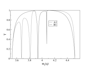
Figure 4: Transmission coefficient versus $\omega_{3}(q)$ with Fano resonances for waves scattered by A-type (dashed) and B-type (solid) DBs with one vertical resistive junction for $\Omega_{b}=3.1$, $\beta_{L}=0.5$ and $\eta=0.35$.

The number of localized modes of the dc part of the scattering potential does not change when the damping and bias become nonzero. But in this case there are two dispersion curves with nonzero dispersion $\omega_{2,3}(q)$. One of them is located above the plasma frequency $|\omega_{1}(q)|<|\omega_{3}(q)|$ (as before) and the second one below it $|\omega_{2}(q)|<|\omega_{1}(q)|$. Since the latter one possesses a rather weak dispersion, for small damping $\alpha\approx 0.01$ there are still localized modes, which satisfy the condition (17).

We also incorporated the finite damping into the calculation of the transmission coefficient by using the transformation (3). The resulting scattering problem can be again analyzed along the lines of the Floquet approach from above. Note that this modified scheme implies the excitation of a scattering wave setup which decays in time in a spatial homogeneous way. The numerical results of this scheme for $\alpha=0.01$ coincide with the transmission shown in Fig. 4. The Fano resonance positions are practically the same, because the frequencies of localized modes almost did not change.

VIII.2 Direct numerical simulations

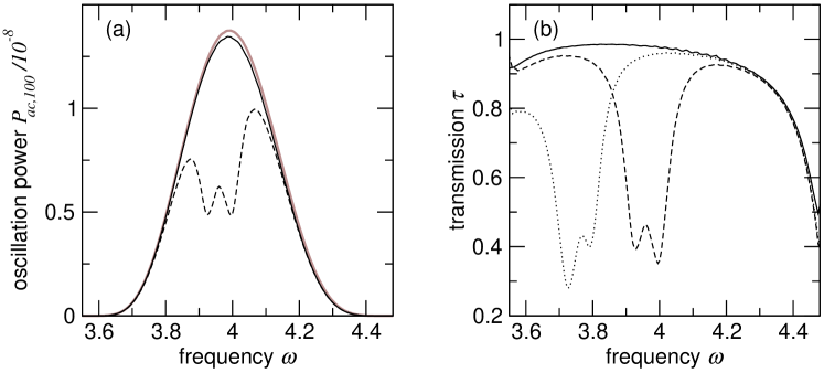
Figure 5: Direct numerical simulation of the linear wave propagation in a JJL with $N=100$ cells, $\alpha=0.05$, $\beta_{L}=0.5$, $\eta=0.35$ with a boundary ac bias $\gamma_{1}=\gamma_{\text{ac}}\cos(\omega t)$. (a) Oscillation power of vertical junction $n=101$ versus excitation frequency $\omega$ for an empty system (solid grey line), for an A DB at site $n=50$ with frequency $\Omega_{b}=2.777$ (solid line), and $\Omega_{b}=3.284$ (dashed line). (b) Transmission coefficient $\tau$ for an A DB of frequency $\Omega_{b}=2.777$ (solid line), $\Omega_{b}=3.284$ (dashed line), and frequency $\Omega=3.082$ (dotted line).

.

In order to test whether the Fano resonances computed along the lines of the Floquet approach (see Fig. 4) also persist in an experimental situation, we performed direct numerical simulations of the scattering of linear waves by a DB in Josephson ladders which emulate a real experimental situation. The equations of motion were numerically integrated using a standard fifth order Runge Kutta scheme press97:_numer with precision monitoring. To study the scattering of linear waves by a DB in a situation comparable to an experiment, a special scattering experiment scheme was set up. Linear waves are generated in a JJL with open ends by locally applying a time-periodic current $\gamma_{1}(t)$ at the vertical junction $1$: $\gamma_{1}(t)=\gamma_{ac}\cos(\omega t).$ The local current acts as a local parametric drive. It excites a tail of junctions that oscillate with frequency $\omega$. This tail extends into the ladder and decays exponentially in space. The situation is comparable to a DB with frequency $\omega$ located at the system boundary. In Refs. flach99:_rotob_josep ; aemsfmvfyzjbp01 , the spatial extent of oscillatory tails of DBs was computed analytically. If the frequency $\omega$ lies inside the dispersive $\omega_{3}$ band, the tail decays as $\varphi_{n}\propto\exp(-\alpha n)$. Outside the band, the oscillations practically do not penetrate into the system. To monitor the linear wave propagation in the system, we compute the time-averaged oscillation power of vertical junction $n$, $P_{\text{ac},n}=\langle\dot{\varphi}_{n}^{2}\rangle$.

As a scatterer, a DB of either type A or B is launched in the center of the system. The DB frequency is then tuned by a spatially uniform DC bias $\gamma$.

We simulate an open-ended JJL with $N=100$ cells, damping $\alpha=0.05$, discreteness $\beta_{L}=0.5$, and anisotropy $\eta=0.35$. The vertical junction at the left edge $n=1$ is driven by a time-dependent current with $\gamma_{\text{ac}}=0.05$. The driving frequency is swept within $3\leq\omega\leq 5$. At each frequency step, the system is integrated over a time period of $500$ units to allow for relaxation. The dynamical values are then monitored over the following $300$ time units. During that time the oscillation power and phase velocities are averaged and recorded.

Fig. 5(a) displays the obtained average oscillation power spectrum in the vertical junction $n=101$ (at the right edge of the ladder which is opposite to the ac-driven junction). In the empty case without a scattering DB state inside the ladder, the oscillation power shows a broad peak when the excitation frequency $\omega$ is inside the $\omega_{3}$ band. Outside the band, the oscillations quickly decay to a level below $10^{-20}$. As a test, the frequency-dependent spatial decay was compared to the analytical predictions and perfect agreement was found. When a scattering DB is inserted into the system at the central site $n=50$, the propagation of linear waves is modified, and dips may appear in the power spectrum (dashed line in Fig. 5.

We obtain the transmission coefficient $\tau$ by relating the oscillation power at the boundary vertical junction ($n=101$) with and without a DB inside the system, as

$$\tau\equiv\frac{P_{\text{ac},101}(\text{with DB})}{P_{\text{ac},101}(\text{without DB})}.$$ (18)

Figure 6: Dip frequency $\omega_{\text{dip}}$ in the transmission from Fig. 5(b) versus DB frequency $\Omega$ for a type A DB (two dips, marked by circles and squares) and a type B DB (one dip, diamonds). Lines indicate linear fits of the dip frequency to Eq. (19).

Fig. 5(b) shows the obtained transmission for type A scatterer states. Outside the $\omega_{3}$ band, linear waves do not propagate, hence any obtained transmission coefficient is meaningless. Inside the band, we show the transmission through DBs of three different frequencies. In the first case of small DB frequency $\Omega_{b}=2.777$, the transmission curve has a broad maximum. The DB is practically transparent in the center of the $\omega_{3}$ band. If we increase the frequency of the scattering DB, dips appear in the transmission at frequencies $\omega_{\text{dip}}$. The values of these frequencies change upon variation of the scatterer DB frequency $\Omega_{b}$.

We systematically varied the scattering DB frequency and computed various transmission curves. In Fig. 6, we show the dependence of the positions of the dips in the spectrum $\omega_{\text{dip}}$ as a function of the scattering DB frequency $\Omega_{b}$ for type A and type B states. The obtained dependence is linear and follows

$$\omega_{\text{dip}}=A_{0}+A_{1}\Omega_{b}.$$ (19)

For the type A scattering DB, two dips were observed. For the lower one we find $A_{0}=0.601$ and $A_{1}=1.015$ from a least squares fit, while the upper resonance satisfies $A_{0}=0.680$ and $A_{1}=1.009$. In the case of a B type DB, we observe only one resonance, following $A_{0}=0.995$ and $A_{1}=0.966$. We interpret $A_{0}$ as the frequency of a dc local mode, while $A_{1}$ is practically equal to unity, and find perfect agreement with Eq. (17). We thus conclude that the dips in the transmission spectrum are in fact Fano resonances.

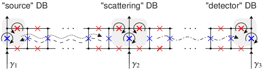
Figure 7: Schematic experimental setup for measuring the plasmon scattering by a DB, showing source, scattering, and detector DB. The individual DBs are controlled using local bias currents $\gamma_{1}$–$\gamma_{3}$. Technical details are found in Ref. msdiss04 .

The persistence of the Fano resonance in the direct simulations of the finite size Josephson ladder including damping gives a strong indication for a possible experimental observation of the phenomenon. Experimentally, the time-dependent local biasing of one ladder end requires microwaves. However, instead of using an external source, a resonant DB state, as studied experimentally in Ref. schuster01:_obser_josep , could be used to create linear waves. A scattering setup should therefore consist of a resonant DB state used as an emitter (creating linear waves), while another (non-resonant) DB within a suitable distance would act as a scatterer. For the detection of radiation we suggest the use of another set of resistive Josephson junctions inside the ladder, situated at the far end. These junctions may be seen again as a DB state. Their property of quasi-particle detection can be then used by biasing them close to the superconducting gap voltage dayem . Fig. 7 gives a sketch of the experimental setup of locally biased DB states used as linear wave source, scatterer, and detector. Promising experimental studies are under way (see Ref. msdiss04 for details).

IX Conclusion

We investigate theoretically the existence of Fano resonances in wave scattering by DBs in JJLs. Due to the weak coupling between open and closed channels of the scattering potential, generated by a DB, perfect reflection occurs, according to the theory in the Hamiltonian limit, when multiples of frequency of DBs match the difference between the frequency of a dc local mode and some frequency in the spectrum. Numerical calculations of the transmission coefficient based on the Floquet approach confirm this analytical prediction. Moreover, Fano resonances survive even the presence of dissipation and external dc bias. Direct numerical simulations of the damped and biased system demonstrate Fano resonances as well. This is a strong indication that Fano resonances can be observed experimentally in Josephson junction ladders.

An interesting question is why the direct numerical simulations do not show a perfect reflection (cf. Fig. 5), at variance with the computation of the transmission coefficient based on the Floquet approach (cf. Fig. 4). We checked that this is neither an artifact of the numerics, nor due to finite size effects. The two methods (direct simulations and Floquet based approach) differ in the way boundary conditions are defined. The only explanation we thus arrive at, is that although the damping is weak, it leads to a different damping of the propagating waves in different channels. Waves propagating locally around the breather at different frequencies (i.e. in different channels) are damped at a different rate, which depends on the frequency of oscillations. Correspondingly the phase and amplitude relations between the partial waves in different channels are changed, leading only to a partial destructive interference gurvitz92 . Alternative explanations involve the broadening of a resonance frequency line due to damping. The damping causes the transmission to stay nonzero in the resonance, and changes (broadens) the line width of the resonance. This also leads to the impossibility of resolving two closely nearby lying resonances, exactly as we found in our numerical studies for the type B breather.

Fano resonances can be considered as a benchmark of dynamical localized excitations (DBs) in their action on propagating waves in the system. A similar proposal for the observation of Fano resonances in light-light scattering in nonlinear optical media has been reported in Ref.gorbach .

Acknowledgements
We thank R. Pinto for a careful reading of the manuscript. M.V.F. thanks the financial support of SFB 491.

Appendix A Appendix A: Dispersion of linear waves

Substituting the expressions (2) into system (II) together with the transformation (3) and linearizing with respect to the small excitations, we obtain

$$\ddot{\psi}_{n}^{v}+(\sqrt{1-\gamma^{2}}-\frac{\alpha^{2}}{4})\psi_{n}^{v} = \frac{1}{\beta_{L}}(\triangle\psi_{n}^{v}+\nabla\psi_{n-1}^{h}-\nabla\tilde{\psi}_{n-1}^{h})$$

$$\ddot{\psi}_{n}^{h}+(1-\frac{\alpha^{2}}{4})\psi_{n}^{h} = -\frac{1}{\eta\beta_{L}}(\nabla\psi_{n}^{v}+\psi_{n}^{h}-\tilde{\psi}_{n}^{h})$$ (20)

$$\ddot{\tilde{\psi}}{}_{n}^{h}+(1-\frac{\alpha^{2}}{4})\tilde{\psi}^{h}_{n} = \frac{1}{\eta\beta_{L}}(\nabla\psi_{n}^{v}+\psi_{n}^{h}-\tilde{\psi}_{n}^{h})\;.$$

By using the plane wave ansatz

$$\vec{\psi}_{n}={\mathrm{e}}^{{\mathrm{i}}(qn-\omega_{q}t)}\vec{A}_{q}\;,$$ (21)

one obtains that there are three bands. One of them is dispersionless

$$\omega_{1}^{2}(q)=1-\frac{\alpha^{2}}{4}\;.$$ (22)

For $\alpha=0$ this is the plasma frequency and it is characterized by in-phase excitations of upper and lower horizontal junctions $A^{h}=\tilde{A}^{h}$ and all vertical junctions being at rest $A^{v}=0$. Due to the absence of dispersion this mode can be excited in each cell with arbitrary amplitudes, since it does not propagate along the ladder.

The two other bands are located above and below it

$$\omega_{2,3}(q)^{2}=F\mp\sqrt{F^{2}-G}\;,$$

$$F = \frac{1}{2}+\frac{1}{\beta_{L}\eta}+\frac{1}{2}\sqrt{1-\gamma^{2}}+\frac{1}{\beta_{L}}(1-\cos q)-\frac{\alpha^{2}}{4}\;,$$

$$G = (1+\frac{2}{\beta_{L}\eta}-\frac{\alpha^{2}}{4})(\sqrt{1-\gamma^{2}}-\frac{\alpha^{2}}{4})+$$

$$+\frac{2}{\beta_{L}}(1-(1+\frac{\alpha^{2}}{4})\cos q-\frac{\alpha^{2}}{4})\;.$$

The dispersion of the second band $\omega_{2}(q)$ is weak. The polarization vectors of these two branches can be written in a compact form

$$A^{h}=-\tilde{A}^{h}\;,\;A^{h}=\frac{{\mathrm{e}}^{{\mathrm{i}}q}-1}{\beta_{L}\eta(1-\omega_{2,3}^{2}(q)-\alpha^{2}/4)+2}A^{v}$$ (24)

In the Hamiltonian limit $\alpha=0$ and $\gamma=0$ the band $\omega^{2}_{2}(q)=1$ becomes dispersionless as well. Its polarization vectors are simplified to out-of-phase excitations of upper and lower horizontal junctions $A^{h}=-\tilde{A}_{h}$ and $A^{h}=\frac{1}{2}(1-{\mathrm{e}}^{{\mathrm{i}}q})A^{v}$. The third band $\omega_{3}(q)$ keeps a finite dispersion

$$\omega^{2}_{3}(q)=1+\frac{2}{\beta_{L}\eta}+\frac{2}{\beta_{L}}(1-\cos q)$$ (25)

with corresponding in-phase excitations of upper and lower horizontal junctions and the following relation between vertical and horizontal ones

$$A^{h}=\tilde{A}^{h}\;\;,\;\;\;A^{v}=\eta({\mathrm{e}}^{-{\mathrm{i}}q}-1)A_{h}\;.$$ (26)

References

- (1) A. J. Sievers and J. B. Page, in: Dynamical properties of solids VII phonon physics the cutting edge, Elsevier, Amsterdam (1995); S. Aubry, Physica D 103, 201 (1997); S. Flach, C.R. Willis, Phys. Rep. 295, 181 (1998); Energy Localisation and Transfer, Eds. T. Dauxois, A. Litvak-Hinenzon, R. MacKay and A. Spanoudaki, World Scientific (2004); D. K. Campbell, S. Flach and Yu. S. Kivshar, Physics Today, p.43, January 2004.
- (2) E. Trias, J. J. Mazo, and T. P. Orlando, Phys. Rev. Lett. 84, 741 (2000); P. Binder, D. Abraimov, A. V. Ustinov, S. Flach, and Y. Zolotaryuk, Phys. Rev. Lett. 84, 745 (2000); A. Ustinov. Chaos 13, 716 (2003).
- (3) H. S. Eisenberg et al., Phys. Rev. Lett. 81, 3383 (1998); R. Morandotti et al., Phys. Rev. Lett. 83, 2726 (1999); 83, 4756 (1999); J. W. Fleischer, M. Segev, N. K. Efremidis, and D. N. Christodoulides, Nature 422, 147 (2003); D.Cheskis et.al., Phys. Rev. Lett. 91, 223901 (2003).
- (4) B. Swanson et al., Phys. Rev. Lett. 82, 3288 (1999); K. Kladko, J. Malek, and A. R. Bishop, J. Phys.: Condens. Matter 11, L415 (1999).
- (5) U.T. Schwarz, L.Q. English, and A.J. Sievers, Phys. Rev. Lett. 83, 223 (1999); M. Sato and A. J. Sievers, Nature 432, 486 (2004).
- (6) M. Sato, B. E. Hubbard, A. J. Sievers, B. Ilic, D. A. Czaplewski, and H. G. Craighead, Phys. Rev. Lett. 90, 044102 (2003); M. Sato, B. E. Hubbard, A. J. Sievers et al., Europhys. Lett. 66, 318 (2004).
- (7) B. Eiermann, Th. Anker, M. Albiez, M. Taglieber, P. Treutlein, K.-P. Marzlin, and M. K. Oberthaler, Phys. Rev. Lett. 92, 230401 (2004).
- (8) M. Machida and T. Koyama, Phys. Rev. B 70, 024523 (2004).
- (9) I. Kourakis and P. K. Shukla, Phys. Plasmas 12, 014502 (2005).
- (10) T. Cretegny, S. Aubry, and S. Flach, Physica D 119, 73 (1998).
- (11) S. W. Kim and S. Kim, Physica D 141, 91 (2000).
- (12) S. W. Kim and S. Kim, Phys. Rev. B 63, 212301 (2001).
- (13) S. Flach, A. E. Miroshnichenko and M. V. Fistul, Chaos 13, 596 (2003).
- (14) S. Flach, A. E. Miroshnichenko, V. Fleurov, and M. V. Fistul, Phys. Rev. Lett. 90, 084101 (2003).
- (15) U. Fano, Phys.Rev. 124, 1866 (1961); J.A. Simpson and U. Fano, Phys. Rev. Lett. 11, 158 (1963).
- (16) L. M. Floria, J. L. Marin, P. J. Martinez, F. Falo, and S. Aubry, Europhys. Lett. 36, 539 (1996); J. J. Mazo, E. Trias, and T. P. Orlando, Phys. Rev. B 59, 13604 (1999); P. Binder, D. Abraimov, and A. V. Ustinov, Phys. Rev. E 62 2858 (2000); M. V. Fistul, A. E. Miroshnichenko, S. Flach, M. Schuster, and A. V. Ustinov, Phys. Rev. B 65, 174524 (2002); P. Binder and A. V. Ustinov, Phys. Rev. E 66, 016603 (2002); .
- (17) E. Trias, J. J. Mazo, A. Brinkman, and T. P. Orlando, Physica D 156, 98 (2001).
- (18) A. E. Miroshnichenko, S. Flach, M. V. Fistul, Y. Zolotaryuk, and J. B. Page, Phys. Rev. E, 64, 066601 (2001).
- (19) A. E. Miroshnichenko, S. Flach, and B. Malomed, Chaos 13, 874 (2003).
- (20) S. Flach and M. Spicci, J. Phys: Condens. Matter 11, 321 (1999).
- (21) M. Schuster, P. Binder, and A. V. Ustinov, Phys. Rev. E 65, 016606 (2001).
- (22) W. H. Press, Numerical Recipes in C, The Art of Scientific Computing, second ed., Cambridge University Press, 1997.
- (23) A. H. Dayem and R. J. Martin, Phys. Rev. Lett. 8, 246 (1962).
- (24) M. Schuster, PhD Thesis, University of Erlangen (2004).
- (25) S. A. Gurvitz and Y. B. Levinson, Phys. Rev. B 47, 10578 (1992).
- (26) S. Flach, V. Fleurov, A. Gorbach, and A. M. Miroshnichenko, nlin.PS/0409023 (2004).