Abstract

We introduce the stochastic multiplicative point process modelling trading activity of financial markets. Such a model system exhibits power-law spectral density $S(f)\propto 1/f^{\beta}$ , scaled as power of frequency for various values of $\beta$ between 0.5 and 2. Furthermore, we analyze the relation between the power-law autocorrelations and the origin of the power-law probability distribution of the trading activity. The model reproduces the spectral properties of trading activity and explains the mechanism of power-law distribution in real markets.

Keywords: financial markets, stochastic modelling, point processes, 1/f noise.
PACS: 05.40.-a, 02.50.Ey, 89.65.Gh

1 Introduction

Power-laws are intrinsic features of the economic and financial data. There are numerous studies of power-law probability distributions in various economic systems [1, 2, 3, 4, 5, 6, 7, 8]. The key result in recent findings is that the cumulative distributions of returns and trading activity can be well described by a power-law asymptotic behavior, characterized by an exponent $\lambda\approx 3$, well outside the Levy stable regime $0<\lambda<2$ [8].

The time-correlations in the financial time series are studied extensively as well [8, 9, 10]. Gopikrishnan et al [8, 9] provided empirical evidence that the long-range correlations for volatility were due to the trading activity, measured by a number of transactions $N$.

Recently we adapted the model of $1/f$ noise based on the Brownian motion of time interval between subsequent pulses, proposed in [11, 12, 13, 14], to model the share volume traded in the financial markets [15]. The idea to transfer long time correlations into the stochastic process of the time interval between trades or time series of trading activity is in consistence with the detailed studies of the empirical financial data [8, 9] and fruitfully reproduces the spectral properties of the financial time series [15, 16]. Further, we generalized the model defining stochastic multiplicative point process to reproduce a variety of self-affine time series exhibiting the power spectral density $S(f)$ scaling as a power of frequency, $S(f)\propto f^{-\beta}$ [17].

In this contribution we analyze the applicability of the stochastic multiplicative point process as a model of trading activity in the financial markets. We investigate the spectral density and counting statistics of model trading activity in comparison with empirical data from the stock exchange. The model reproduces the spectral properties of trading activity and explains the mechanism of power law distribution in the real markets.

2 The model

We consider a point process $I(t)$ as a sequence of the $\delta$-type random correlated pulses,

$$I(t)=\sum\limits_{k}a_{k}\delta(t-t_{k}),$$ (1)

and define the number of trades $N_{j}$ in the time intervals $\tau_{d}$ as an integral of the signal, $N_{j}=\int\limits_{t_{j}}^{t_{j}+\tau_{d}}I(t)dt$. Here $a_{k}$ is a contribution of one transaction. When $a_{k}=1$, the signal (1) counts the transactions in the financial market. When $a_{k}$ describes asset price change during one transaction, the signal counts the price changes. When $a_{k}=\bar{a}$ is a constant, the point process is completely described by the set of times of the events $\{t_{k}\}$ or equivalently by the set of interevent intervals $\{\tau_{k}=t_{k+1}-t_{k}\}$. Various stochastic models for $\tau_{k}$ can be introduced to define a stochastic point process. In papers [11, 12, 13, 14] it has been shown analytically that the relatively slow Brownian fluctuations of the interevent time $\tau_{k}$ yield $1/f$ fluctuations of the signal (1). In [17] we have generalized the model introducing stochastic multiplicative process for the interevent time $\tau_{k}$,

$$\tau_{k+1}=\tau_{k}+\gamma\tau_{k}^{2\mu-1}+\tau_{k}^{\mu}\sigma\varepsilon_{k}.$$ (2)

Here the interevent time $\tau_{k}$ fluctuates due to the external random perturbation by a sequence of uncorrelated normally distributed random variable $\{\varepsilon_{k}\}$ with zero expectation and unit variance, $\sigma$ denotes the standard deviation of the white noise and $\gamma\ll 1$ is a damping constant. From the big variety of possible stochastic processes we have chosen the multiplicative one, which yields multifractal intermittency and power-law probability distribution functions. Pure multiplicativity corresponds to $\mu=1$. Other values of $\mu$ may be considered, as well.

The iterative relation (2) can be rewritten as Langevine stochastic differential equation in $k$-space

$$\frac{d\tau_{k}}{dk}=\gamma\tau_{k}^{2\mu-1}+\tau_{k}^{\mu}\sigma\xi\left(k\right).$$ (3)

Here we interpret $k$ as continuous variable while $\left\langle\xi\left(k\right)\xi\left(k^{\prime}\right)\right\rangle=\delta(k-k^{\prime})$.

The steady state solution of the stationary Fokker-Planck equation with zero flow, corresponding to (3), gives the probability density function for $\tau_{k}$ in the $k$-space (see, e.g., [18])

$$P_{k}(\tau_{k})=C\tau_{k}^{\alpha}=\frac{\alpha+1}{\tau_{max}^{(\alpha+1)}-\tau_{min}^{(\alpha+1)}}\tau_{k}^{\alpha},\quad\alpha=2\gamma/\sigma^{2}-2\mu.$$ (4)

The steady state solution (4) assumes Ito convention involved in the relation between expressions (2), (3) and (4) and the restriction for the diffusion $0<\tau_{\min}<\tau_{k}<\tau_{\max}$.

We have already derived the formula for the power spectral density of the multiplicative stochastic point process model, defined by Eqs. (2) and (3) for the interevent time [17],

$$S_{\mu}(f)=\frac{2C\overline{a}^{2}}{\sqrt{\pi}\overline{\tau}(3-2\mu)f}\left(\frac{\gamma}{\pi f}\right)^{\frac{\alpha}{3-2\mu}}{\mathop{\mathrm{Re}}}\int\limits_{x_{\min}}^{x_{\max}}\exp\left\{-i\bigg{(}x-\frac{\pi}{4}\bigg{)}\right\}{\mathop{\mathrm{erfc}}}(\sqrt{-ix})x^{\frac{\alpha}{3-2\mu}-\frac{1}{2}}dx$$ (5)

where $\bar{\tau}=\left\langle\tau_{k}\right\rangle=T/(k_{\max}-k_{\min})$ is the expectation of $\tau_{k}$. Here we introduce the scaled variable $x=\pi f\tau^{3-2\mu}/\gamma$ and $x_{\min}=\pi f\tau_{\min}^{3-2\mu}/\gamma,\quad x_{\max}=\pi f\tau_{\max}^{3-2\mu}/\gamma$.

Expression (5) is appropriate for the numerical calculations of the power spectral density of the generalized multiplicative point process defined by Eqs. (1) and (2). In the limit $\tau_{\min}\rightarrow 0$ and $\tau_{\max}\rightarrow\infty$ we obtain an explicit expression

$$S_{\mu}(f)=\frac{C\overline{a}^{2}}{\sqrt{\pi}\overline{\tau}(3-2\mu)f}\left(\frac{\gamma}{\pi f}\right)^{\frac{\alpha}{3-2\mu}}\frac{\Gamma(\frac{1}{2}+\frac{\alpha}{3-2\mu})}{\cos(\frac{\pi\alpha}{2(3-2\mu)})}.$$ (6)

Equation (6) reveals that the multiplicative point process (2) results in the power spectral density $S(f)\sim 1/{f^{\beta}}$ with the scaling exponent

$$\beta=1+\frac{2\gamma/\sigma^{2}-2\mu}{3-2\mu}.$$ (7)

Let us compare our analytical results (5) and (6) with the numerical calculations of the power spectral density according to equations (1) and (2). In Fig. 1 we present the numerically calculated power spectral density $S(f)$ of the signal $I(t)$ for $\mu=0.5$ and $\alpha=2\gamma/\sigma^{2}-1=0$, -0.5 and +0.5. Numerical results confirm that the multiplicative point process exhibits the power spectral density scaled as $S(f)\sim 1/f^{\beta}$. Equation (5) describes the model power spectral density very well in a wide range of parameters. The explicit formula (6) gives a good approximation of power spectral density for the parameters when $\beta\simeq 1$. These results confirm the earlier finding [11, 12, 13, 14] that the power spectral density is related to the probability distribution of the interevent time $\tau_{k}$ and $1/f$ noise occurs when this distribution is flat, i.e., when $\alpha=0$.

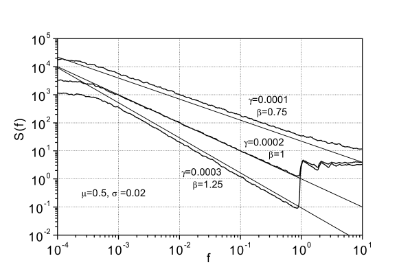
Figure 1: Power spectral density $S(f)$ vs frequency $f$ calculated numerically according to Eqs. (1) and (2) with the parameters $\mu=0.5$, $\sigma=0.02$ and different relaxations of the signal $\gamma$. We restrict the diffusion of the interevent time in the interval $\tau_{min}=10^{-6}$; $\tau_{max}=1$ with the reflective boundary condition at $\tau_{min}$ and transition to the white noise, $\tau_{k+1}=\tau_{max}+\sigma\varepsilon_{k}$, for $\tau_{k}>\tau_{max}$. The straight lines represent the results given by the explicit formula (6).

It is likely that such a stochastic model with parameters in the region $0.5\leq\beta\leq 1.5$ may be adaptable for a wide variety of different systems. In this paper we will discuss applicability of the model for the financial market.

We derived pdf of $N$ for the pure multiplicative model with $\mu=1$ in [17]

$$P(N)=\frac{C^{\prime}\tau_{d}^{2+\alpha}(1+\gamma N)}{N^{3+\alpha}(1+\frac{\gamma}{2}N)^{3+\alpha}}\sim\left\{\begin{array}[]{ll}\frac{1}{N^{3+\alpha}},&N\ll\gamma^{-1},\\ \frac{1}{N^{5+2\alpha}},&N\gg\gamma^{-1}.\end{array}\right.$$ (8)

Probability distribution function for $N$ obtained from the numerical simulation of the model is in a good agreement with the analytical result (8).

3 Discussion and conclusions

We have introduced a multiplicative stochastic model for the time intervals between events of point process. Such a model of time series has only a few parameters defining the statistical properties of the system, i.e., the power-law behavior of the distribution function and the scaled power spectral density of the signal. The ability of the model to simulate $1/f$ noise as well as to reproduce signals with the values of power spectral density slope $\beta$ between 0.5 and 1.5 promises a wide variety of applications of the model.

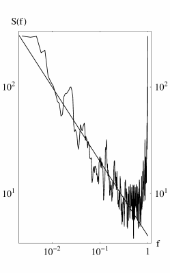
Figure 2: Power spectral density $S(f)$ vs frequency $f$ calculated numerically from the empirical data of 3 most liquid stocks from the Lithuanian Stock Exchange. Straight line fits $S(f)\propto f^{-0.7}$.

Let us present shortly the possible interpretations of the empirical data of the trading activity in the financial markets. With a very natural assumption of transactions in the financial markets as point events we can model the number of transactions $N_{j}$ in equal time intervals $\tau_{d}$ as the outcome of the described multiplicative point process. We already know from available studies [8] that the empirical data exhibit power spectral density in the low frequency limit with the slope $\beta\simeq 0.7$. Empirical data from the Lithuanian Stock Exchange for the most liquid assets confirm the same value $\beta\simeq 0.7$, (see Fig 2). For the pure multiplicative model with $\mu=1$ this results in $\alpha=2\gamma/\sigma^{2}-2\mu\simeq-0.3$. The corresponding cumulative distribution of $N$ in the tail of high values (see equation (8)) has the exponent $\lambda=4+2\alpha=3.4$. This is in an excellent agreement with the empirical cumulative distribution exponent 3.4 defined in [8] for 1000 stocks of the three major US stock markets.

The numerical results confirm that the multiplicative stochastic model of the time interval between trades in the financial market is able to reproduce the main statistical properties of trading activity $N$ and its power spectral density. The power-law exponents of the pdf of the interevent time, $\alpha$, and the cumulative distribution of the trading activity, $\lambda$, as well as the slope of power spectral density, $\beta$, are defined just by one parameter of the model $2\gamma/\sigma^{2}$. The model suggests a simple mechanism of the power-law statistics of trading activity in the financial markets.

References

- [1] M. Levy, S. Solomon, Int. J. Mod. Phys. C 7 (1996) 595.
- [2] M. Levy, S. Solomon, Physica A 242 (1997) 90.
- [3] D. Sornette, R. Cont, J. Phys. I (France) 7 (1997) 431.
- [4] P. Gopikrishnan et al., Eur. Phys. J. B 3 (1998) 139.
- [5] A. Blank, S. Solomon, Physica A 287 (2000) 279.
- [6] P. Richmond, Eur. Phys. J. B 20 (2001) 523.
- [7] J.P. Bouchaud, e-print: cond-mat/0008103, 2000.
- [8] P. Gopikrishnan et al., Physica A 287 (2000) 362.
- [9] P. Gopikrishnan et al., Phys. Rev. E 62 (2000) R4493.
- [10] P. Cizeau, et al., Quant. Finance 1 (2001) 217.
- [11] B. Kaulakys, T. Meškauskas, Phys. Rev. E 58 (1998) 7013.
- [12] B. Kaulakys, Phys. Lett. A 257 (1999) 37.
- [13] B. Kaulakys, T. Meškauskas, Nonlin. Anal.: Mod. Contr., Vilnius 4 (1999) 87.
- [14] B. Kaulakys, Microel. Reliab. 40 (2000) 1787; cond-mat/0305067, 2003.
- [15] V. Gontis, Lithuanian J. Phys. 41 (2001) 551; cond-mat/0201514, 2002.
- [16] V. Gontis, Nonlin. Anal.: Mod. Contr. 7 (2002) 43; cond-mat/0211317, 2002.
- [17] V. Gontis, B. Kaulakys, Proc. 17th ICNF, Prague 2003, p.622-625; cond-mat/0303089, 2002.
- [18] C.W. Gardiner, Handbook of Stochastic Methods, Springer, Berlin, 1986.