Twist of cholesteric liquid crystal cells:
stability of helical structures and anchoring energy effects

Abstract

We consider helical configurations of a cholesteric liquid crystal (CLC) sandwiched between two substrates with homogeneous director orientation favored at both confining plates. We study the CLC twist wavenumber $q$ characterizing the helical structures in relation to the free twisting number $q_{0}$ which determines the equilibrium value of CLC pitch, $P_{0}=2\pi/q_{0}$. We investigate the instability mechanism underlying transitions between helical structures with different spiral half-turn numbers. Stability analysis shows that for equal finite anchoring strengths this mechanism can be dominated by in-plane director fluctuations. In this case the metastable helical configurations are separated by the energy barriers and the transitions can be described as the director slippage through these barriers. We extend our analysis to the case of an asymmetric CLC cell in which the anchoring strengths at the two substrates are different. The asymmetry introduces two qualitatively novel effects: (a) the intervals of twist wavenumbers representing locally stable configurations with adjacent helix half-turn numbers are now separated by the instability gaps; and (b) sufficiently large asymmetry, when the difference between azimuthal anchoring extrapolation lengths exceeds the thickness of the cell, will suppress the jump-like behaviour of the twist wavenumber.

I Introduction

In equilibrium cholesteric phase molecules of a liquid crystal (LC) align on average along a local unit director $\mathbf{n}(\mathbf{r})$ that rotates in a helical fashion about a uniform twist axis de Gennes and Prost (1993). This tendency of cholesteric liquid crystals (CLC) to form helical twisting patterns is caused by the presence of anisotropic molecules with no mirror plane — so-called chiral molecules (see Harris et al. (1999) for a recent review).

The phenomenology of CLCs can be explained in terms of the Frank free energy density

$$f_{b}[\mathbf{n}]=\frac{1}{2}\Bigl{\{}K_{1}({\nabla}\cdot\mathbf{n})^{2}+K_{2}\left[\mathbf{n}\cdot{\nabla\times\mathbf{n}}+q_{0}\right]^{2}$$

$$+K_{3}\,[\mathbf{n}\times(\nabla\times\mathbf{n})]^{2}-K_{24}\mathop{\rm div}\nolimits\left(\mathbf{n}\mathop{\rm div}\nolimits\mathbf{n}+\mathbf{n}\times(\nabla\times\mathbf{n})\right)\Bigr{\}}\,,$$ (1)

where $K_{1}$, $K_{2}$, $K_{3}$ and $K_{24}$ are the splay, twist, bend and saddle-splay Frank elastic constants. As an immediate consequence of the broken mirror symmetry, the expression for the bulk free energy (1) contains a chiral term proportional to the equilibrium value of the CLC twist wavenumber, $q_{0}$.

The parameter $q_{0}$, which will be referred to as the free twist wavenumber or as the free twisting number, gives the equilibrium helical pitch $P_{0}\equiv 2\pi/q_{0}$. For the twist axis directed along the $z$-direction, the director field $\mathbf{\hat{n}}=(\cos q_{0}z,\sin q_{0}z,0)$ then defines the equilibrium configuration in an unbounded CLC. Periodicity of the spiral is given by the half-pitch, $P_{0}/2$, because $\mathbf{\hat{n}}$ and $-\mathbf{\hat{n}}$ are equivalent in liquid crystals,

Typically, the pitch $P_{0}$ can vary from hundreds of nanometers to many microns or more, depending on the system. The macroscopic chiral parameter, $h=q_{0}K_{2}$, (and thus the pitch) is determined by microscopic intermolecular torques Harris et al. (1997); Lubensky et al. (1997) and depends on the molecular chirality of CLC consistuent mesogens. The microscopic calculations of the chiral parameter are complicated as it is necessary to go beyond the mean-field approach and to take into account biaxial correlations Harris et al. (1999). Despite recent progress Emelyanenko et al. (2000); Emelyanenko (2003), this problem has not been resolved completely yet.

In this paper we are primarily concerned with orientational structures in planar CLC cells bounded by two parallel substrates. Director configurations in such cells are strongly affected by the anchoring conditions at the boundary surfaces which break the translational symmetry along the twisting axis. So, in general, the helical form of the director field will be distorted.

Nevertheless, when the anchoring conditions are planar and out-of-plane deviations of the director are suppressed, it might be expected that the configurations still have the form of the ideal helical structure. But, by contrast with the case of unbounded CLCs, the helix twist wavenumber $q$ will now differ from $q_{0}$.

It has long been known that a mismatch between the equilibrium pitch $P_{0}$ and the twist imposed by the boundary conditions may produce two metastable twisting states that are degenerate in energy and can be switched either way by applying an electric field Berreman and Heffner (1981). This bistability underlines the mode of operation of bistable liquid crystal devices — the so-called bistable twisted nematics — that have been attracted considerable attention over past few decades Xie and Kwok (1998); Zhuang et al. (1999); Xie et al. (2000); Fion and Kwok (2003).

More generally the metastable twisting states in CLC cells appear as a result of interplay between the bulk and the surface contributions to the free energy giving rise to multiple local minima of the energy. The purpose of this paper is to explore the multiple minima and their consequences.

The free twisting number $q_{0}$ and the anchoring energy are among the factors that govern the properties of the multiple minima representing metastable states. Specifically, varying $q_{0}$ will change the twist wavenumber of the twisting state, $q$. This may result in sharp transitions between different branches of metastable states. The dependence of the twist wavenumber $q$ on the free twisting number $q_{0}$ is then discontinuous. As far as we are aware, attention was first drawn to this phenomenon by Reshetnyak et. al Pinkevich et al. (1992).

These discontinuities are accompanied by a variety of physical manifestations which have been the subject of much recent important research. One such is a jump-like functional dependence of selective light transmission spectra on temperature as a result of a temperature-dependent cholesteric pitch, examined by Zink and Belyakov Zink and Belyakov (1997, 1999). More recently Belyakov et. al Belyakov and Kats (2000); Belyakov et al. (2003) and Palto Palto (2002) have discussed different mechanisms behind temperature variations of the pitch in CLC cells and hysteresis phenomena.

In this paper we adapt a systematic approach and study the helical structures using stability analysis. This approach enables us to go beyond the previous work by relaxing a number of constraints. One of these requires anchoring to be sufficiently weak (where “sufficiently” will be discussed further below), so that the jumps may occur only due to transitions between the helical configurations which numbers of spiral half-turns differ by the unity Belyakov and Kats (2000); Belyakov et al. (2003). Noticeably, this assumption eliminates important class of the transitions that involve topologically equivalent structures with the half-turn numbers of the same parity.

We shall also apply our theory to the case of non-identical confining plate and show that asymmetry in the anchoring properties of the bounding surfaces results in qualitatively new effects. Specifically, we find that sufficiently large asymmetry in anchoring strengths will suppress the jump-like behaviour of the twist wavenumber $q$ when the free wavenumber $q_{0}$ varies.

The layout of the paper is as follows. General relations that determine the characteristics of the helical structures in CLC cells are given in Sec. II. Then in Sec. III we outline the procedures which we use to study stability of the director configurations. The stability analysis is performed for in-plane and out-of-plane fluctuations invariant with respect to in-plane translations. We study CLC cells with the strong anchoring conditions and the cases where at least one anchoring strength is finite. We formulate the stability conditions and the criterion for the stability of the helical structures to be solely governed by the in-plane director fluctuations. The expressions for the fluctuation static correlation functions are given. In Sec. IV we study the dependence of the twist wavenumber on the free twisting number. Finally, in Sec. V we present our results and make some concluding remarks. Details on some technical results are relegated to Appendix A.

II Helical structures

II.1 Energy

We consider a CLC cell of thickness $d$ sandwiched between two parallel plates that are normal to the $z$-axis: $z=-d/2$ and $z=d/2$. Anchoring conditions at both substrates are planar with the preferred orientation of CLC molecules at the lower and upper plates defined by the two vectors of easy orientation: $\mathbf{\hat{e}}_{-}$ and $\mathbf{\hat{e}}_{+}$. These vectors are given by

$$\mathbf{e}_{-}=\mathbf{e}_{x},\quad\mathbf{e}_{+}=\cos\Delta\phi\,\mathbf{e}_{x}+\sin\Delta\phi\,\mathbf{e}_{y},$$ (2)

where $\Delta\phi$ is the twist angle imposed by the boundary conditions.

We shall also write the elastic free energy as a sum of the bulk and surface contributions:

$$F[\mathbf{n}]=\int_{V}f_{b}[\mathbf{n}]\,\mathrm{d}v+\sum_{\nu=\pm 1}\int_{z=\nu d/2}W_{\nu}(\mathbf{n})\,\mathrm{d}s$$ (3)

and assume that both the polar and the azimuthal contributions to the anchoring energy $W_{\nu}(\mathbf{n})$ can be taken in the form of Rapini-Papoular potential Rapini and Papoular (1969):

$$W_{\nu}(\mathbf{n})=\frac{W^{(\nu)}_{\phi}}{2}\Bigl{[}1-\bigl{(}{\mathbf{n}},{\mathbf{e}_{\nu}}\bigr{)}^{2}\Bigr{]}_{z=\nu d/2}+\frac{W^{(\nu)}_{\theta}}{2}\Bigl{[}1-\bigl{(}{\mathbf{n}},{\mathbf{e}_{z}}\bigr{)}^{2}\Bigr{]}_{z=\nu d/2},$$ (4)

where $W^{(\pm)}_{\phi}$ and $W^{(\pm)}_{\theta}$ are the azimuthal and the polar anchoring strengths.

The CLC helical director structures take the following spiral form

$$\mathbf{n}_{0}=\cos u(z)\,\mathbf{e}_{x}+\sin u(z)\,\mathbf{e}_{y},\quad u(z)=qz+\phi_{0},$$ (5)

where $q$ is the twist (or pitch) wavenumber and $\phi_{0}$ is the twist angle of the director in the middle of the cell. The configurations (5) can be obtained as a solution of the Euler-Lagrange equations for the free energy functional (1) provided the invariance with respect to translations in the $x-y$ plane is unbroken.

The translation invariant solutions can be complicated by the presence of the out-of-plane director deviations neglected in Eq. (5) and, in general, does not represent a helical structure. Using Eq. (5) is justified only for those configurations that are stable with respect to out-of-plane director fluctuations. The corresponding stability conditions will be derived in the next section.

We can now substitute Eq. (5) into Eq. (3) to obtain the following expression for the rescaled free energy per unit area of the director configuration (5):

$$(2d/K_{2})F[\mathbf{n}_{0}]\equiv f[\mathbf{n}_{0}]=(qd-q_{0}d)^{2}+2\sum_{\nu=\pm 1}w^{(\nu)}_{\phi}\sin^{2}u_{\nu},$$ (6)

where $u_{\nu}$ is the angle between the vector of easy orientation $\mathbf{e}_{\nu}$ and the director $\mathbf{n}_{0}$ at the plate $z=\nu d/2$; and the dimensionless azimuthal anchoring energy parameter $w^{(\nu)}_{\phi}$ is proportional to the ratio of the cell thickness, $d$, and the azimuthal extrapolation length, $L^{(\nu)}_{\phi}=W^{(\nu)}_{\phi}/K_{2}$:

$$w^{(\nu)}_{\phi}\equiv\frac{W^{(\nu)}_{\phi}d}{2K_{2}}=\frac{d}{2L^{(\nu)}_{\phi}},\quad\cos u_{\nu}\equiv\bigl{(}{\mathbf{n}_{0}},{\mathbf{e}_{\nu}}\bigr{)}\Bigr{|}_{z=\nu d/2}.$$ (7)

The energy (6) is of the well-known “smectic-like” form de Gennes and Prost (1993) and can be conveniently rewritten in terms of the following dimensionless parameters

$$\beta=qd-\Delta\phi,\quad\beta_{0}=q_{0}d-\Delta\phi,\quad\alpha=2\phi_{0}-\Delta\phi$$ (8)

by using the relations

$$d(q-q_{0})=\beta-\beta_{0},\quad 2u_{\nu}=\nu\beta+\alpha.$$ (9)

Given the free twist parameter $\beta_{0}$ the energy (6) is now a function of $\alpha$ and the twist parameter $\beta$ which characterize the helical structure (5). The azimuthal angles of the director at the bounding surfaces, $\phi_{\nu}=u(\nu d/2)$, can be expressed in terms of the parameters (8) and $\Delta\phi$ as follows

$$\phi_{+}=u_{+}+\Delta\phi=(\beta+\alpha)/2+\Delta\phi,\quad\phi_{-}=u_{-}=(-\beta+\alpha)/2.$$ (10)

II.2 Twist wavenumber and parity

It is not difficult to show that in order for the configuration to be an extremal of the free energy (3) these parameters need to satisfy the system of the following two equations:

$$\beta_{0}=\beta+w^{(\nu)}_{\phi}\sin(\beta+\nu\alpha),\quad\nu=\pm 1.$$ (11)

Equivalently, this system determines the extremals as stationary points of the energy (6) and can be derived from the condition that both energy derivatives with respect to $\alpha$ and $\beta$ vanish.

Eq. (11) can now be used to relate the parameters $\alpha$ and $\beta$ through the equation

$$\alpha=\arctan[\epsilon\tan\beta]+\pi k,\quad\epsilon\equiv\frac{w^{(-)}_{\phi}-w^{(+)}_{\phi}}{w^{(-)}_{\phi}+w^{(+)}_{\phi}},$$ (12)

where $k$ is the integer, $k\in\mathbb{Z}$, that defines the parity of the configuration $\mu=(-1)^{k}$.

Indeed, substituting Eq. (12) into Eq. (11) gives the relation between $\beta_{0}$ and $\beta$

$$\beta_{0}=\gamma_{\mu}(\beta)\equiv\beta+\mu w^{(+)}_{\phi}\sin(\beta+\arctan[\epsilon\tan\beta]),\quad\mu=(-1)^{k},$$ (13)

that depends on $k$ only through the parity. This remark also applies to the expression for the energy that after substituting the relation (12) into Eq. (6) can be recast into the form

$$f_{\mu}(\beta)=\bigl{[}w^{(+)}_{\phi}\sin v_{+}\bigr{]}^{2}+(w^{(+)}_{\phi}+w^{(-)}_{\phi})-\mu\sum_{\nu=\pm 1}w^{(\nu)}_{\phi}\cos v_{\nu},$$ (14)

where

$$v_{\nu}=\beta+\nu\arctan[\epsilon\tan\beta].$$ (15)

In Sec. IV we will find that there are different branches of metastable helical configurations. Each branch is characterized by the number of the spiral half-turns and $\mu$ is the parity of this number. For this reason, the integer $k$ will be referred to as the half-turn number.

Thus, we have classified the director structures by means of the parity $\mu$ and the dimensionless twist parameter $\beta$ that can be computed by solving the transcendental equation (13). Fig. 1 illustrates the procedure of finding the roots of Eq. (13) in the $\beta-\gamma$ plane.

In general, there are several roots represented by the intersection points of the horizontal line $\gamma=\beta_{0}$ and the curves $\gamma=\gamma_{\pm}(\beta)$. Each root corresponds to the director configuration which energy can be calculated from Eq. (14). The equilibrium director structure is then determined by the solution of Eq. (13) with the lowest energy. Other structures can be either metastable or unstable.

II.3 Strong anchoring limit

However, these results cannot be applied directly to the case of the strong anchoring limit, where $W^{(\nu)}_{\phi}\to\infty$ and the boundary condition requires the director at the substrate $z=\nu d/2$ to be parallel to the corresponding easy axis, $\mathbf{n}(\nu d/2)\parallel\mathbf{e}_{\nu}$.

When the anchoring is strong at both substrates, it imposes the restriction on the values of $q$, so that $q$ takes the values from a discrete set de Gennes and Prost (1993). This set represents the director configurations characterized by the parameter $\beta$ and labelled by the half-turn number $k$

$$\beta\equiv qd-\Delta\phi=\pi k,\quad k\in\mathbb{Z}\,.$$ (16)

Substituting the values of $\beta$ from Eq. (16) into the first term on the right hand side of Eq. (6) will define the equilibrium value of $k$ as the integer that minimizes the distance between $\pi k$ and $\beta_{0}$ ($=q_{0}d-\Delta\phi$). The step-like dependence of $\beta$ on $\beta_{0}$ for these equilibrium structures is depicted in Fig. 2(a).

An experimentally important case concerns mixed boundary conditions in which the strong anchoring limit applies to the lower plate only, $W^{(-)}_{\phi}\to\infty$. For brevity, this case will be referred to as the semi-strong anchoring. Now the relations (12) and (13) reduce to

$$\alpha=\beta+2\pi k,$$ (17)

$$\beta_{0}=\beta+w^{(+)}_{\phi}\sin(2\beta)$$ (18)

and the energy of the helical structures (14) is now given by

$$f(\beta)=\bigl{[}w^{(+)}_{\phi}\sin(2\beta)\bigr{]}^{2}+2w^{(+)}_{\phi}\sin^{2}\beta.$$ (19)

Interestingly, in the semi-strong anchoring limit, the parity of half-turns, $\mu$, does not enter either the energy (19) or the relation (18).

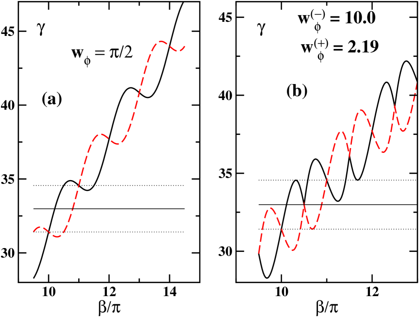
Figure 1: The curves representing the plot of the function $\gamma_{+}(\beta)$ and $\gamma_{-}(\beta)$ are shown as thick solid and dashed lines, respectively. The points located at the intersection of the curves and the horizontal straight line $\gamma=\beta_{0}$ give the roots of Eq. (13). The value of $\beta_{0}$ is $(10+1/2)\pi$ (thin solid line) and is $(10+1/2)\pi\pm w_{\phi}$ (thin dotted lines). Two cases are illustrated: (a) $w^{(+)}_{\phi}=w^{(-)}_{\phi}=w_{\phi}=\pi/2$; (b) $w^{(-)}_{\phi}=10.0$, $w^{(+)}_{\phi}=2.19$, $w_{\phi}=\pi/2$ (see Eq. (56)).

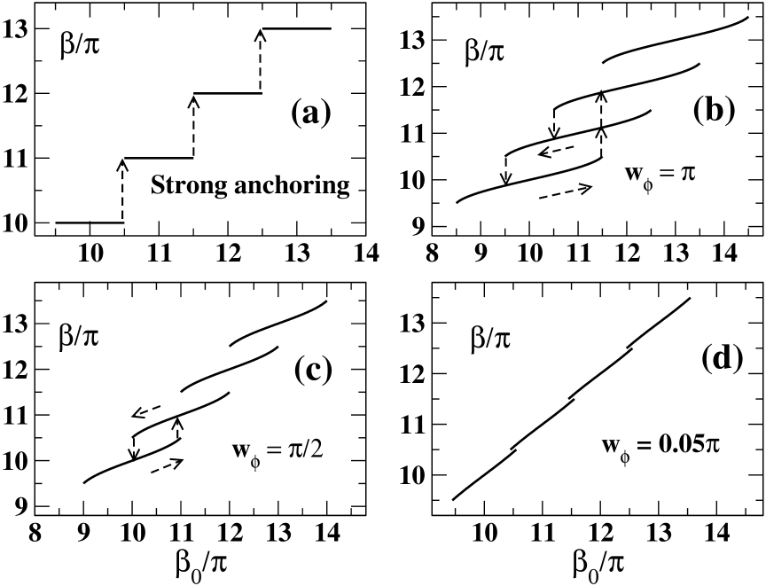
Figure 2: Dependence of the twist parameter $\beta$ ($=qd-\Delta\phi$) on the free twisting parameter $\beta_{0}$ ($=q_{0}d-\Delta\phi$) at $W^{(-)}_{\phi}=W^{(+)}_{\phi}\equiv W_{\phi}$ for various values of the dimensionless azimuthal anchoring parameter $w_{\phi}$ ($=W_{\phi}d/2K_{2}$): (a) strong anchoring limit, $w_{\phi}\to\infty$, discussed in Sec. II.3; (b) $w_{\phi}=\pi$; (c) $w_{\phi}=\pi/2$; (d) $w_{\phi}=0.05\pi$. Discussion of the cases (b)-(d) can be found in Sec. IV.1.

III Stability of helical structures

In this section we present the results on stability of the helical configurations (5). These results then will be used in Sec. IV to eliminate unstable structures from consideration. We also give expressions for director correlation functions. These are in order to discuss the effects of director fluctuations.

We begin with the general expression for the distorted director field

$$\mathbf{n}=\cos\theta\cos\phi\,\mathbf{n}_{0}+\cos\theta\sin\phi\,\mathbf{n}_{1}+\sin\theta\,\mathbf{n}_{2},\quad\bigl{(}{\mathbf{n}_{i}},{\mathbf{n}_{j}}\bigr{)}=\delta_{ij},$$ (20)

where the vectors $\mathbf{n}_{1}$ and $\mathbf{n}_{2}$ are

$$\mathbf{n}_{1}=-\sin u(z)\,\mathbf{e}_{x}+\cos u(z)\,\mathbf{e}_{y},\quad\mathbf{n}_{2}=\mathbf{e}_{z}.$$ (21)

For small angles $\phi$ and $\theta$ linearization of Eq. (20) gives the perturbed director field in the familiar form

$$\mathbf{n}\approx\mathbf{n}_{0}+\delta\mathbf{n}_{0},\quad\delta\mathbf{n}_{0}=\phi\,\mathbf{n}_{1}+\theta\,\mathbf{n}_{2},\quad\boldsymbol{\psi}\equiv\begin{pmatrix}\phi\\ \theta\end{pmatrix},$$ (22)

where the angles $\phi$ and $\theta$ describe in-plane and out-of-plane deviations of the director, respectively.

Following standard procedure, we can now expand the free energy of the director field (20) up to second order terms in the fluctuation field $\boldsymbol{\psi}$ and its derivatives

$$F[\mathbf{n}]\approx F[\mathbf{n}_{0}]+F^{(2)}[\boldsymbol{\psi}],$$ (23)

$$F^{(2)}[\boldsymbol{\psi}]=\int_{V}f_{b}^{(2)}[\boldsymbol{\psi}]\,\mathrm{d}v+\sum_{\nu=\pm 1}\int_{z=\nu d/2}W_{\nu}^{(2)}(\boldsymbol{\psi})\,\mathrm{d}s.$$ (24)

The second order variation of the free energy $F^{(2)}[\boldsymbol{\psi}]$ is a bilinear functional which represents the energy of the director fluctuations written in the harmonic (Gaussian) approximation. ¿From Eqs. (1)-(3) we obtain expressions for the densities that enter the fluctuation energy (24):

$$2f^{(2)}_{b}[\boldsymbol{\psi}]=K_{1}\bigl{(}\nabla_{1}\phi+\nabla_{2}\theta\bigr{)}^{2}+K_{2}\bigl{(}\nabla_{1}\theta-\nabla_{2}\phi\bigr{)}^{2}$$

$$+K_{3}\bigl{[}(\nabla_{0}\phi)^{2}+(\nabla_{0}\theta)^{2}\bigr{]}+qK_{q}\bigl{[}2\theta\,\nabla_{0}\phi+q\theta^{2}\bigr{]},$$ (25)

$$2W^{(2)}_{\nu}(\boldsymbol{\psi})=\Bigl{[}W^{(\nu)}_{\phi}\phi^{2}\cos 2u_{\nu}+W^{(\nu)}_{\theta}\theta^{2}$$

$$-2\nu K_{24}\,\theta\,\nabla_{1}\phi\Bigr{]}_{z=\nu d/2},\;$$ (26)

where $\nabla_{i}\equiv\bigl{(}{\mathbf{n}_{i}},{\boldsymbol{\nabla}}\bigr{)}$.

In what follows we shall restrict our consideration to the case of fluctuations invariant with respect to in-plane translations, so that $\boldsymbol{\psi}\equiv\boldsymbol{\psi}(z)$. This assumption, although restricting applicability of our results, allows us to avoid complications introduced by inhomogeneity of the helical structure (5). In this case the fluctuation energy per unit area is

$$2F^{(2)}[\boldsymbol{\psi}]/S=\int_{-d/2}^{d/2}{\boldsymbol{\psi}}^{+}\,\hat{K}\boldsymbol{\psi}\,\mathrm{d}z+\sum_{\nu=\pm 1}{\boldsymbol{\psi}}^{+}\,\hat{Q}^{(\nu)}\boldsymbol{\psi}\Bigr{|}_{z=\nu d/2},$$ (27)

where $S$ is the area of the substrates. The operator $\hat{K}$ is the differential matrix operator that enters the linearized Euler-Lagrange equations for the director distribution (20), i.e.

$$\hat{K}\boldsymbol{\psi}=0.$$ (28)

The eigenvalues of $\hat{K}$ form the fluctuation spectrum Kiselev (2004). The eigenvalues $\lambda$ can be computed together with the eigenmodes $\boldsymbol{\psi}_{\lambda}$ by solving the boundary-value problem:

$$\hat{K}\boldsymbol{\psi}_{\lambda}=\lambda\boldsymbol{\psi}_{\lambda},$$ (29)

$$\hat{Q}^{(\nu)}\boldsymbol{\psi}_{\lambda}\Bigr{|}_{z=\nu d/2}=0.$$ (30)

The expressions for $\hat{K}$ and $\hat{Q}^{(\nu)}$ are given by

$$\hat{K}=\begin{pmatrix}-K_{2}\partial_{z}^{2}&0\\ 0&-K_{1}\partial_{z}^{2}+q^{2}K_{q}\end{pmatrix},$$ (31)

$$\hat{Q}^{(\nu)}= \nu\begin{pmatrix}K_{2}\partial_{z}&0\\ 0&K_{1}\partial_{z}\end{pmatrix}$$

$$+\begin{pmatrix}W^{(\nu)}_{\phi}\cos 2u_{\nu}&0\\ 0&W^{(\nu)}_{\theta}\end{pmatrix},$$ (32)

and $K_{q}$ is the effective elastic constant

$$K_{q}=K_{3}-2K_{2}(1-q_{0}/q).$$ (33)

¿From Eqs. (31)-(III) the operators $\hat{K}$ and $\hat{Q}^{(\nu)}$ are both diagonal, so that the in-plane and out-of-plane fluctuations are statistically independent and can be treated separately.

III.1 In-plane fluctuations

III.1.1 Strong and semi-strong anchoring

We begin with the limiting cases discussed in Sec. II.3 and where at least one of the bounding surfaces imposes the strong anchoring boundary condition. This is the case when we have to use stability criterion related to the fluctuation spectrum which requires all the eigenvalues to be positive, $\lambda>0$, as to ensure the positive definiteness of the fluctuation energy Kiselev (2004).

It is not difficult to see that, for the strong azimuthal anchoring present at both substrates, the lowest eigenvalue is

$$\lambda_{m}=K_{2}(\pi/d)^{2}$$ (34)

and all the structures with the twist parameter (16) are locally stable with respect to in-plane fluctuations.

For the semi-strong anchoring with $W^{(-)}_{\phi}\to\infty$, this is no longer the case. The stability condition is now given by

$$1+2w^{(+)}_{\phi}\cos(2\beta)>0.$$ (35)

¿From Eq. (18) this condition requires the free twist parameter $\beta_{0}$ to be an increasing function of the twist parameter $\beta$. It is derived in Appendix A [see Eq. (73) with $w_{+}$ replaced by $w^{(+)}_{\phi}\cos(2\beta)$].

III.1.2 Weak anchoring

We have a somewhat different situation when the azimuthal anchoring strength is finite at both substrates. In this case the stability conditions can be derived using an alternative procedure Kiselev (2004). The procedure involves two steps: (a) solving the linearized Euler-Lagrange equations (28); and (b) substituting the general solution into the expression for the fluctuation energy (27). The last step gives the energy (27) expressed in terms of the integration constants, so that the stability conditions can be derived as conditions for this expression to be positive definite.

Following this procedure, we can obtain the stability conditions for the helical structures characterized by the parity $\mu$ and the twist parameter $\beta$ related to the free twist parameter $\beta$ through the relation (13). The final result is

$$H_{\mu}=A_{\mu}+2w^{(+)}_{\phi}w^{(-)}_{\phi}\cos v_{+}\cos v_{-}>0,$$ (36)

$$A_{\mu}=\mu(w^{(+)}_{\phi}\cos v_{+}+w^{(-)}_{\phi}\cos v_{-})>0,$$ (37)

where $v_{\pm}$ are defined in Eq. (15). These inequalities also follow immediately from the stability conditions (72) obtained in Appendix A by putting $w_{\pm}=\mu w^{(\pm)}_{\phi}\cos v_{\pm}$.

Violating either of Eqs. (35)-(37) will result in instability caused by slippage of the director in the plane of the spiral. Such an instability cannot occur when the azimuthal anchoring is strong at both substrates.

III.2 Out-of-plane fluctuations

We now study stability of the helical structures with respect to the out-of-plane fluctuations. To this end we replace $\lambda$ with $K_{1}(2/d)^{2}\lambda$ and rewrite the eigenvalue problem (29)-(30) for $\theta$ in the following form:

$$\bigl{[}\partial_{\tau}^{2}-r_{q}/4+\lambda\bigr{]}\,\theta_{\lambda}(\tau)=0,$$ (38)

$$\Bigl{[}\pm\partial_{\tau}\theta_{\lambda}+w^{(\pm)}_{\theta}\theta_{\lambda}\Bigr{]}_{\tau=\pm 1}=0,$$ (39)

$$r_{q}=(qd)^{2}K_{q}/K_{1}=(\beta+\Delta\phi)\bigl{(}r_{3}(\beta+\Delta\phi)+2r_{2}(\beta_{0}-\beta)\bigr{)},$$ (40)

$$w^{(\nu)}_{\theta}\equiv\frac{W^{(\nu)}_{\theta}d}{2K_{1}}=\frac{d}{2L^{(\nu)}_{\theta}},$$ (41)

where $\tau\equiv 2z/d$, $r_{i}\equiv K_{i}/K_{1}$ and $L^{(\nu)}_{\theta}$ is the polar anchoring extrapolation length.

The stability condition $\lambda>0$ can now be readily written as follows

$$4\lambda_{m}+r_{q}>0,$$ (42)

where $\lambda_{m}$ is the lowest eigenvalue of the problem (38)-(39) computed at $r_{q}=0$.

When the polar anchoring is strong at both substrates, $W^{(\pm)}_{\theta}\to\infty$, the eigenvalue $\lambda_{m}$ is known [see remark at the end of Appendix A]:

$$\lambda_{m}=(\kappa_{m})^{2}=\pi^{2}/4.$$ (43)

Otherwise, $\kappa_{m}$ is below $\pi/2$ and can be computed as the root of the transcendental equation deduced in Appendix A [see Eq. (74)]

$$D(\kappa_{m})\equiv(w^{(+)}_{\theta}w^{(-)}_{\theta}-\kappa_{m}^{2})\sin 2\kappa_{m}+\kappa_{m}(w^{(+)}_{\theta}+w^{(-)}_{\theta})\cos 2\kappa_{m}=0,$$ (44)

where $0\leq\kappa_{m}<\pi/2$.

III.2.1 Strong anchoring

In the strong anchoring limit, Eq. (16) implies that the values of the twist parameter $\beta$ are quantized and do not depend on the free twist parameter $\beta_{0}$. Unstable configurations are characterized by twist wavenumbers violating the stability condition (42) with $\lambda_{m}$ given in Eq. (43). These wavenumbers are described by the inequalities

$$1/\tilde{\beta}_{-}\leq 1/\tilde{\beta}\leq 1/\tilde{\beta}_{+},\quad\tilde{\beta}\equiv qd/\pi,\;\tilde{\beta}_{0}\equiv q_{0}d/\pi,$$

$$1/\tilde{\beta}_{\pm}=-r_{2}\tilde{\beta}_{0}\pm\bigl{[}(r_{2}\tilde{\beta}_{0})^{2}+2r_{2}-r_{3}\bigr{]}^{1/2}.$$ (45)

These inequalities yield two different sets of unstable structures depending on the sign of the difference $(2K_{2}-K_{3})$. For $q_{0}\geq 0$ these sets are given by

$$2K_{2}>K_{3}:$$

$$q\geq(\pi/d)|\tilde{\beta}_{+}|\;\text{ or }\;q\leq-(\pi/d)|\tilde{\beta}_{-}|,$$ (46)

$$K_{3}>2K_{2}:$$

$$-(\pi/d)|\tilde{\beta}_{+}|\leq q\leq-(\pi/d)|\tilde{\beta}_{-}|\;\text{ at }\;q_{0}\geq\pi/(dr_{2})\sqrt{r_{3}-2r_{2}}.$$ (47)

Eq. (III.2.1) shows that, when the energy cost of bend is relatively small, there are an infinite number of unstable configurations and the configuration loses its stability as the distance between its wavenumber $q$ and $q_{0}$ becomes sufficiently large.

Otherwise, unstable configurations may appear only if the free wavenumber $q_{0}$ exceeds its critical value given in Eq. (III.2.1). In this case the number of the unstable configurations is finite. From Eq. (III.2.1) there is no unstable configurations for nematic liquid crystals with $q_{0}=0$. This result has been previously reported in Ref. Goldbart and Ao (1990).

III.2.2 Weak anchoring

We now pass on to the case where the strengths of anchoring $W^{(\pm)}_{\phi}$ are not infinitely large. By contrast to the case of strong anchoring, the twist parameters $\beta$ and $\beta_{0}$ are now not independent. Rather we have the stationarity condition (13) relating $\beta$ and $\beta_{0}$. In addition, if the polar anchoring is also not infinitely strong, the eigenvalue $\lambda_{m}$ can be considerably reduced.

In these circumstances, it is reasonable to approximate the left hand side of the stability condition (42) by its lower bound derived in the limit of weak polar anchoring, $W^{(\nu)}_{\theta}\to 0$, where $\lambda_{m}$ vanish. Technically, the resulting condition

$$r_{q}(\beta,\mu)=(\beta+\Delta\phi)\bigl{(}\,2\,r_{2}\,\beta_{0}(\beta,\mu)+(r_{3}-2r_{2})\beta+r_{3}\Delta\phi\,\bigr{)}>0$$ (48)

is sufficient but not necessary for stability. Thus, when the inequality (48) is satisfied, the structure will certainly be locally stable with respect to out-of-plane fluctuations whatever the polar anchoring is.

Eq. (48) can now be used to study out-of-plane fluctuation induced instability of the helical structures which are otherwise stable with respect to in-plane fluctuations and thus meet the stability conditions (36)-(37). For $\Delta\phi=0$ and positive twist wavenumbers, such instabilty may occur only if the doubled twist elastic constant exceeds the bend elastic constant, $2K_{2}>K_{3}$, and the azimuthal anchoring energy is sufficiently large. In this case, however, $r_{q}$ can be made non-negative by increasing the value of the free twist parameter $\beta_{0}$. In other words, if the ratio of the cell thickness and the equilibrium CLC pitch is large enough to meet the condition (48) we can neglect out-of-plane deviations of the director and use the “smectic-like” free energy (6).

III.3 Correlation functions

Our calculations of the director fluctuation static correlation function $\langle\boldsymbol{\psi}(z)\boldsymbol{\psi}(z^{\prime})\rangle$ use the relation Kiselev (2004)

$$\langle\boldsymbol{\psi}(z)\boldsymbol{\psi}(z^{\prime})\rangle=\frac{k_{B}T}{S}\,\mathbf{G}(z,z^{\prime}),$$ (49)

where $k_{B}$ is the Boltzmann constant and $T$ is the temperature. The Green function $\mathbf{G}(z,z^{\prime})$ can be computed as the inverse of the operator $\hat{K}$ defined in Eq. (31) by solving the boundary-value problem

$$\hat{K}\mathbf{G}(z,z^{\prime})=\delta(z-z^{\prime})\hat{I},$$ (50)

$$\hat{Q}^{(\nu)}\mathbf{G}(z,z^{\prime})\Bigr{|}_{z=\nu d/2}=0,$$ (51)

where $\hat{I}$ is the identity matrix and the operator $\hat{Q}^{(\nu)}$ is given in Eq. (III). Since the matrix operators $\hat{K}$ and $\hat{Q}^{(\nu)}$ are both diagonal, the correlation function (49) is also diagonal:

$$\langle\boldsymbol{\psi}(z)\boldsymbol{\psi}(z^{\prime})\rangle=\begin{pmatrix}\langle\phi(z)\phi(z^{\prime})\rangle&0\\ 0&\langle\theta(z)\theta(z^{\prime})\rangle\end{pmatrix}.$$ (52)

Solving the boundary-value problem (50)-(51) yields the following expressions for the in-plane and the out-of-plane components of the correlation function (52)

$$\langle\theta(z)\theta(z^{\prime})\rangle=\frac{k_{B}Td}{2SK_{1}\kappa D(\kappa)}\,\Bigl{[}w^{(-)}_{\theta}\sin\kappa(1+2z_{<}/d)$$

$$+\kappa\cos\kappa(1+2z_{<}/d)\Bigr{]}\Bigl{[}w^{(+)}_{\theta}\sin\kappa(1-2z_{>}/d)+\kappa\cos\kappa(1-2z_{>}/d)\Bigr{]},$$ (53)

$$\langle\phi(z)\phi(z^{\prime})\rangle=\frac{k_{B}Td}{2SK_{2}H_{\mu}}\,\Bigl{[}1+\mu(1+2z_{<}/d)w^{(-)}_{\phi}\cos v_{-}\Bigr{]}$$

$$\times\Bigl{[}1+\mu(1-2z_{>}/d)w^{(+)}_{\phi}\cos v_{+}\Bigr{]},$$ (54)

where $\kappa^{2}=-r_{q}/4$, $z_{<}\equiv\min\{z,z^{\prime}\}$, $z_{>}\equiv\max\{z,z^{\prime}\}$, $D(\kappa)$ and $H_{\mu}$ are defined in Eq. (44) and Eq. (36), respectively. The correlation functions diverge on approaching the boundary of the stability region. For out-of-plane fluctuations, the denominator of the expression for $\langle\theta(z)\theta(z^{\prime})\rangle$ vanish in the limit of marginal stability where $-r_{q}/4\to\lambda_{m}=\kappa_{m}$ and $D(\kappa)\to D(\kappa_{m})=0$. Similarly, Eq. (36) shows that, in the marginal stability limit for in-plane fluctuations, $H_{\mu}$ goes to zero thus rendering the correlation function $\langle\phi(z)\phi(z^{\prime})\rangle$ divergent.

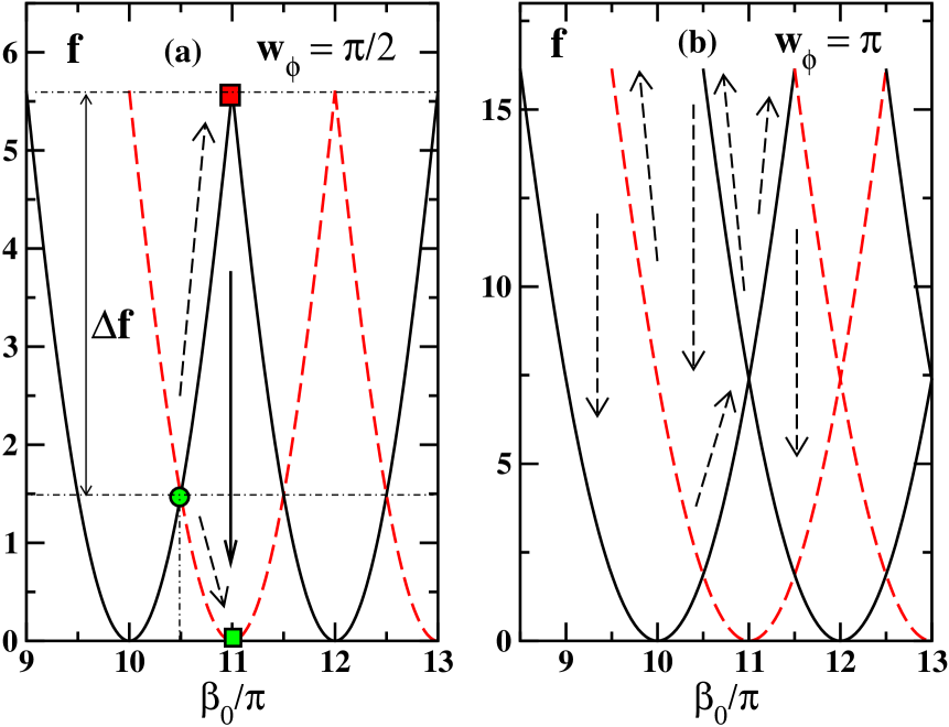
Figure 3: The free energy $f_{+}$ (solid line) and $f_{-}$ (dashed line) of stable configurations with the half-turn number, $k$, between $10$ and $14$ as a function of $\beta_{0}$ computed from Eq. (14) by using Eq. (13) for two values of the anchoring energy parameters: (a) $w_{\phi}=\pi/2$; and (b) $w_{\phi}=\pi$. The intersection point of the branches with $k=10$ and $k=11$ at $\beta_{0}=10.5\pi$ is indicated by circle. Squares mark energy of the structures at the transition point with $\beta_{0}=11\pi$ where the configuration with $k=10$ loses its stability. It is shown that the energy of the helical structure with $k=10$ ($k=11$) increases (decreases) as $\beta_{0}$ varies from $10.5\pi$ to $11\pi$.

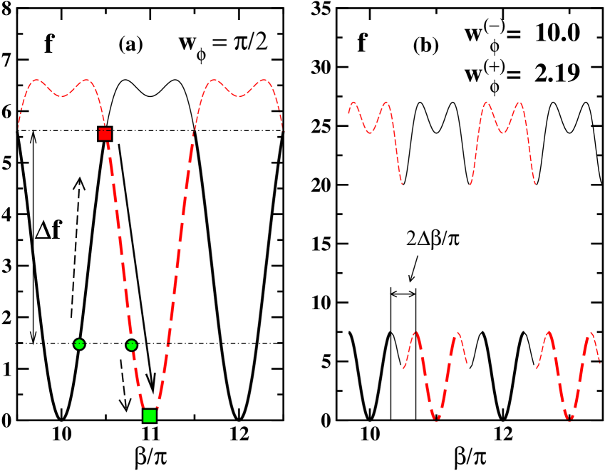
Figure 4: The free energy $f_{+}$ (solid line) and $f_{-}$ (dashed line) of the configurations with the half-turn number, $k$, between $10$ and $14$ as a function of $\beta$ computed from Eq. (14). Thin lines represent the energy of unstable configurations. Two cases are shown: (a) $w^{(-)}_{\phi}=w^{(+)}_{\phi}=w_{\phi}=\pi/2$; and (b) $w^{(-)}_{\phi}=10.0$, $w^{(+)}_{\phi}=2.19$ ($\sigma=5.6$ and $w_{\phi}=\pi/2$). Circles and squares label energy of the structures at $\beta_{0}=10.5\pi$ and $\beta_{0}=11\pi$ shown in Fig. 3(a). At $\beta_{0}=10.5\pi$, the structures with $k=10$ and $k=11$ are shown to be degenerate in energy and separated by the energy barrier $\Delta f$.

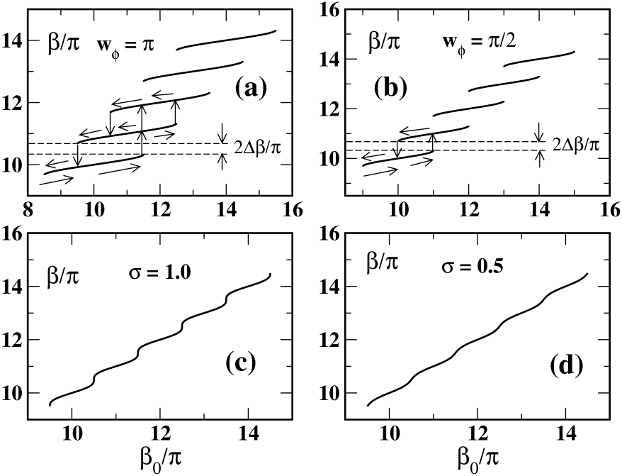
Figure 5: Dependence of $\beta$ on $\beta_{0}$ calculated at $w_{-}=10.0$ for various values of the parameters $\sigma$ ($=2w^{(-)}_{\phi}w^{(+)}_{\phi}/(w^{(-)}_{\phi}-w^{(+)}_{\phi})$) and $w_{\phi}$ (see Eq. (56)): (a) $w_{\phi}=\pi$ ($\sigma=11.8$ and $w^{(+)}_{\phi}=3.705$); (b) $w_{\phi}=\pi/2$ ($\sigma=5.6$ and $w^{(+)}_{\phi}=2.19$); (c) $\sigma=1.0$ ($w^{(+)}_{\phi}=w_{c}=0.476$); (d) $\sigma=0.5$ ($w^{(+)}_{\phi}=0.25$).

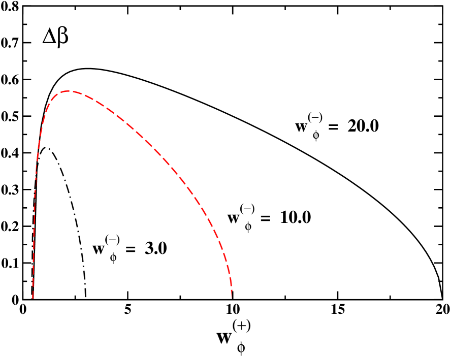
Figure 6: Dependence of $\Delta\beta$ on $w^{(+)}_{\phi}$ for various values of the anchoring energy parameter $w^{(-)}_{\phi}$.

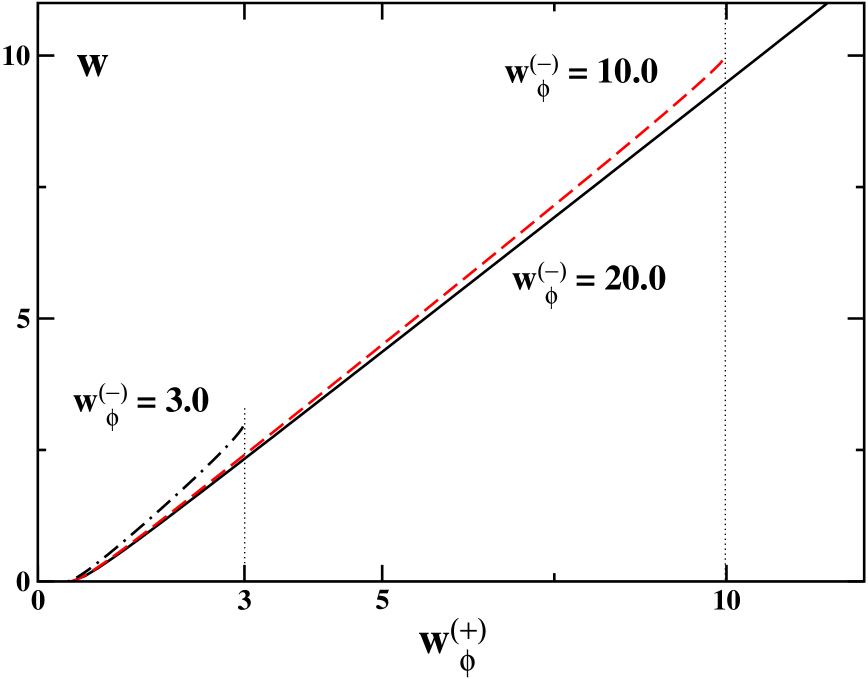
Figure 7: Dependence of $w_{\phi}$ on $w^{(+)}_{\phi}$ for various values of the anchoring energy parameter $w^{(-)}_{\phi}$. It is shown that $w_{\phi}=w^{(-)}_{\phi}$ at $w^{(+)}_{\phi}=w^{(-)}_{\phi}$ and $w_{\phi}=0$ at $w^{(+)}_{\phi}=w_{c}$ (see Eq. (59)).

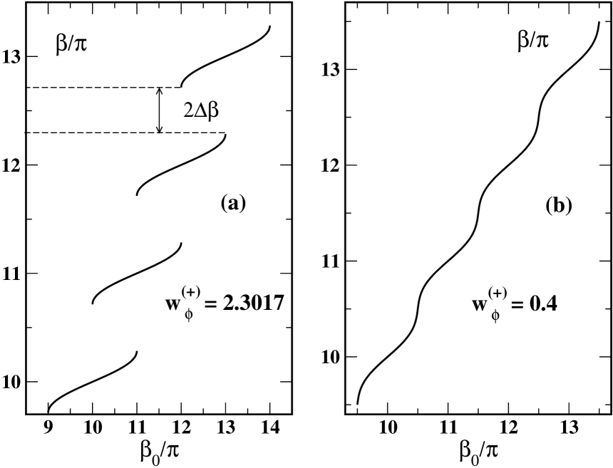
Figure 8: Twist parameter $\beta$ as a function of $\beta_{0}$ in the limit of semi-strong anchoring, $w^{(-)}_{\phi}\to\infty$. Two cases are shown: (a) $w^{(+)}_{\phi}=2.3017>0.5$ with $w_{\phi}=\pi/2$ (see Eq. (61)); and (b) $w^{(+)}_{\phi}=0.4<0.5$.

IV Transitions induced by free wavenumber variations

In the previous section we have studied the stability of the CLC helical structures (5) with respect to both in-plane and out-of-plane fluctuations. We have found that the anchoring conditions play a crucial role in the calculations. In particular, cells with strong anchoring and those with what we have called semi-strong anchoring exhibit significantly different properties.

In this section we concentrate on the weak anchoring cases. We have shown that in this case helical structures are characterized by the twist parameter, $\beta$, and the half-turn parity, $\mu$. These quantities are related to the free twist parameter, $\beta_{0}$, through the stationary point equation (13). The structure responds to variations of the free wavenumber (and thus the free twist parameter) by changing its twist parameter.

This change may render the initially equilibrium structure either metastable or unstable. When the anchoring is not infinitely strong and the free twist parameter is large enough to meet the stability condition (48), this instability is solely governed by in-plane director fluctuations and defines the mechanism dominating transformations of the director field. This mechanism is suppressed in the strong anchoring regime, where the structural transitions involve tilted configurations Goldbart and Ao (1990), and can be described as director slippage through the energy barriers formed by the surface potentials.

In this section our task is to study helical structure transformations as a function of the free twist wavenumber $q_{0}$ for different anchoring conditions. Equivalently, we focus our attention on the dependence of $\beta$ on $\beta_{0}$; this can be thought of as a sort of dispersion relation. To this end we examine in more detail the consequences of the analytical results obtained in the previous sections, Sec. II and Sec. III.

IV.1 Symmetric cells

When the anchoring strengths at both substrates are equal, $W^{(-)}_{\phi}=W^{(+)}_{\phi}\equiv W_{\phi}$, the right hand side of Eq. (13) is $\beta\pm w_{\phi}\sin\beta$ ($w_{\phi}=W_{\phi}d/2K_{2}$) and $v_{\pm}=\beta$. In this case stability of the configurations is governed by Eq. (37) which reduces to the simple inequality $\mu\cos\beta>0$.

It immediately follows that the values of $\beta$ representing the locally stable structures of the parity $\mu$ ranged between $(k-1/2)\pi$ and $(k+1/2)\pi$, where $k$ is the even (odd) integer at $\mu=+1$ ($\mu=-1$). The integer $k$ will be referred to as the half-turn number. The parity $\mu$ introduced in Sec. II is now shown to be the parity of the half-turn number: $\mu=(-1)^{k}$.

The intervals of $\beta$ for the stable configurations $[(k-1/2)\pi,(k+1/2)\pi]$ are now labelled by the half-turn number $k$. Since the function $\gamma_{\mu}$ ($\mu=(-1)^{k}$) monotonically increases on the interval characterized by the half-turn number $k$, the value of $\beta_{0}$ runs from $(k-1/2)\pi-w_{\phi}$ to $(k+1/2)\pi+w_{\phi}$ on this interval. As a result, for each half-turn number $k$, there is the monotonically increasing branch of the $\beta(\beta_{0})$ curve.

The branches with $k$ ranged from $10$ to $13$ for different values of the dimensionless anchoring energy parameter $w_{\phi}$ are depicted in Figs. 2(b)-(d). We see that the $\beta_{0}$-dependence of $\beta$ will always be discontinuous provided the anchoring energy is not equal to zero. Fig. 2(d) shows that the jumps tend to disappear in the limit of weak anchoring, where the azimuthal anchoring energy approaches zero, $w_{\phi}\to 0$.

As we pointed out in Sec. II.3 for the case of strong anchoring, there are two equilibrium structures of the same energy at $\beta_{0}=(1/2+m)\pi$. In Fig. 2(a) the arrows indicate that the half-turn number of the equilibrium structure changes at these points.

Similarly, when the anchoring is weak, $w_{\phi}<\pi$, and $\beta_{0}=(1/2+m)\pi$, Eq. (13) possess two different roots with $k=m$ and $k=m+1$ which are equally distant from $\beta_{0}$ and are of equal energy. In Fig. 3(a), the free energy (14) is shown as a function of $\beta_{0}$. It can be seen that the intersection points of the curves for different parities, (solid and dashed lines in Fig. 3) are indeed at $\beta_{0}=(1/2+m)\pi$. The parity of the equilibrium configuration reverses as $\beta_{0}$ goes through the values $(1/2+m)\pi$. Fig. 3(b) illustrates that this is also the case even if $w_{\phi}\geq\pi$.

For $m=10$, Fig. 3(a) and Fig. 4(a) show the initially equilibrium structure with the half-turn number $k=10$ (solid line) becomes metastable as $\beta_{0}$ passes through the critical point $\beta_{0}=(1/2+m)\pi$ at which the structures with $k=10$ and $k=11$ (dashed line) are degenerate in energy. In Fig. 3(a) and Fig. 4(a) the structures at this point are indicated by circles.

As is seen from the figures, relaxation to the new equilibrium state will require the jump-like change of the twist parameter $\beta$. In addition, the transition between the metastable and the equilibrium configurations involves penetrating the energy barrier $\Delta f$ that separates the states with different half-turn numbers. This barrier can be seen from Figs. 3(a) and 4(a) where the free energy (14) is plotted as a function of $\beta_{0}$ and $\beta$, respectively.

Previous authors Zink and Belyakov (1999); Belyakov and Kats (2000); Palto (2002) have supposed that the transitions may occur only if there is no energy barrier. Clearly, this assumption implies that the jumps take place at the end points of the stability intervals: $\beta_{0}=\beta_{\pm}^{(k)}=(1/2+k)\pi\pm w_{\phi}$, where the configuration with the half-turn number $k$ becomes marginally stable ($A_{\mu}=H_{\mu}=0$) and loses its stability.

These transitions are indicated by arrows in Figs. 2, 3 and 5. As is seen from Fig. 2(c), in this case the upward and backward transitions: $k\to k+1$ and $k+1\to k$ occur at different values of $\beta_{0}$: $\beta_{+}^{(k)}$ and $\beta_{-}^{(k+1)}=\beta_{+}^{(k)}-2w_{\phi}$, respectively. So, there are hysteresis loops in the response of CLC cell to the change in the free twisting number.

We can now describe how the increase in the anchoring energy will affect the scheme of the transitions. To be specific, we consider the critical end point $\beta_{0}=\beta_{+}^{(k)}$, so that for small anchoring energies with $w_{\phi}<\pi/2$ there are only two configurations: the marginally stable initial configuration with $\beta=\beta_{k}$ and the equilibrium structure with $\beta=\beta_{k+1}$. In this case Eq. (13) has at most two roots and the jumps will occur as transitions between the states which half-turn numbers differ by the unity, $|\Delta k|=1$.

At $w_{\phi}=\pi/2$, as shown in Fig. 3(a), we have two marginally stable structures of equal energy: $\beta_{k}$ and $\beta_{k+2}$. The newly formed structure $\beta_{k+2}$ being metastable at $\pi/2<w_{\phi}<\pi$ will have the free energy equal to the energy of the equilibrium configuration $\beta_{k+1}$ at $w_{\phi}=\pi$. So, as illustrated in Figs. 2(b) and 3(b), both transitions $k\to k+1$ and $k\to k+2$ are equiprobable and we have the bistability effect at the critical point under $w_{\phi}=\pi$.

For $\pi<w_{\phi}<3\pi/2$ there are three configurations: the initial configuration $\beta_{k}$, the metastable configuration $\beta_{k+1}$ and the equilibrium structure $\beta_{k+2}$. The configuration $\beta_{k+3}$ being formed at $w_{\phi}=3\pi/2$ will define the equilibrium structure at $2\pi\leq w_{\phi}\leq 3\pi$ and so on.

The general result for the critical point $\beta_{0}=\beta_{+}^{(k)}$ can be summarized as follows. When $(l+1/2)\pi<w_{\phi}<(l+3/2)\pi$, in addition to the marginally stable configuration $\beta_{k}$, there are $l+2$ stable configurations with the half-turn numbers ranged from $k+1$ to $k+l+2$. The half-turn number of the equilibrium structure equals $k+l+1$ under $l\pi<w_{\phi}<(l+1)\pi$.

It immediately follows that the restriction $w_{\phi}<\pi$ imposed by Belyakov and Kats Belyakov and Kats (2000) on the anchoring strength requires the relaxation transitions to involve only two structures with $|\Delta k|=1$. Our result shows that, when the anchoring parameter $w_{\phi}$ falls between $l\pi$ and $(l+1)\pi$, the half-turn number change is $|\Delta k|=l+1$ for the transitions between marginally stable and the equilibrium states. Clearly, we can have the transitions with even $\Delta k$ that involve topologically equivalent configurations with common parity Kléman (1989); Oswald et al. (2000). Such transitions may also be induced by the thermal director fluctuations without formation of defects even if the anchoring is infinitely strong Goldbart and Ao (1990). Though the mechanism under consideration is rather different, neglecting the director fluctuations can only be regarded as a zero-order approximation.

Indeed, according to our remark at the end of Sec. III.2, the expression for the fluctuation correlation function (III.3) implies its divergence upon reaching a marginally stable state where $H_{\mu}=0$. It means that taking the fluctuations into account will give the transition points located within the stability interval. This fluctuation induced shift may also suppress the hysteresis provided the mean square angle deviation $\sqrt{\langle\phi^{2}\rangle}$, computed from Eq. (III.3) at $\beta_{0}=(1/2+m)\pi$ and $z=z^{\prime}=d/2$, and the anchoring energy parameter $w_{\phi}$ are of the same order.

IV.2 Asymmetric cells

When the anchoring energies at the surfaces are different, $W^{(-)}_{\phi}\neq W^{(+)}_{\phi}$ and $\epsilon\neq 0$, $\sin v_{+}$ on the right hand side of Eq. (13) equals zero at $\beta=\pi/2+\pi k$ and, as demonstrated in Fig. 1(b), we have additional intersection points of the curves $\gamma_{+}(\beta)$ and $\gamma_{-}(\beta)$. It can be shown that the stability conditions are now defined by Eq. (36) and the twist parameters $\beta$ of the marginally stable configurations, where $H_{\mu}=0$, can be computed as the stationary points of $\gamma_{\mu}$.

These points represent the local maxima and minima of $\gamma_{\mu}$ and are located at $\beta=(1/2+k)\pi\pm\Delta\beta$. The equation for $\Delta\beta$ is

$$w^{(+)}_{\phi}(1+\epsilon)\sin\bigl{(}\Delta\beta-\epsilon\arctan[\epsilon\cot\Delta\beta]\bigr{)}=-\frac{1+(\epsilon^{2}-1)\cos^{2}\Delta\beta}{1+(\epsilon-1)\cos^{2}\Delta\beta}\,,$$ (55)

where $\Delta\beta\in[0,\pi/2]$.

¿From the stability condition $H_{\mu}>0$ the values of $\beta$ for stable configurations fall between the stationary points $(k-1/2)\pi+\Delta\beta$ and $(k+1/2)\pi-\Delta\beta$, where the half-turn number $k$ is the even (odd) integer depending on the parity. The function $\gamma_{\mu}$ monotonically increases and $\beta_{0}$ varies from $(k-1/2)\pi-w_{\phi}$ to $(k+1/2)\pi+w_{\phi}$ on the stability interval with the half-turn number $k$. The effective dimensionless anchoring parameter $w_{\phi}$, as opposed to the case of equal anchoring energies with $w^{(\pm)}_{\phi}=w_{\phi}$, is now given by

$$w_{\phi}=w^{(+)}_{\phi}\cos\bigl{(}\Delta\beta-\epsilon\arctan[\epsilon\cot\Delta\beta]\bigr{)}-\Delta\beta\,.$$ (56)

Clearly, we can now follow the line of reasoning presented in Sec. IV.1 to find out the results concerning hysteresis loops and bistability effects that are quite similar to the case of equal anchoring strengths (see Figs. 5(a)-(b)). There are, however, two important differences related to Eqs. (55) and (56).

If $\Delta\beta\neq 0$, the intervals of $\beta$ representing stable director configurations are separated by the gap of the length $2\Delta\beta$. The presence of this gap is illustrated in Figs. 5(a) and 5(b). Fig. 4(b) shows the gap between stable branches of the dependence of the free energy on $\beta$. The values of $\beta$ within the gap represent unstable configurations and form the zone of “forbidden” states in the CLC cell.

The graph of the $\Delta\beta$ vs $w^{(+)}_{\phi}$ dependence is presented in Fig. 6. As expected, the gap is shown to disappear in the limit of equal energies, $w^{(+)}_{\phi}=w^{(-)}_{\phi}$. Another and somewhat more interesting effect is that there is a small critical value of $w^{(+)}_{\phi}$ below which $\Delta\beta$ also vanishes.

In order to interpret this effect, we note that Eq. (13) with $\beta_{0}=(1/2+k)\pi$ has the only solution, $\beta=\beta_{0}$, provided the azimuthal anchoring energy parameters meet the condition:

$$\sigma\equiv\frac{2w^{(-)}_{\phi}w^{(+)}_{\phi}}{|w^{(-)}_{\phi}-w^{(+)}_{\phi}|}\leq 1\,.$$ (57)

Another form of this condition

$$|L^{(+)}_{\phi}-L^{(-)}_{\phi}|\geq d$$ (58)

implies that the difference between the azimuthal anchoring extrapolation lengths is larger than the cell thickness. For hybrid cells, similar inequality is known as the stability condition of homogeneous structures Barbero and Barberi (1983); Sparavigna et al. (1994); Ziherl et al. (2000).

In this case the gap disappears and the dependence of $\beta$ on $\beta_{0}$ becomes continuous in the manner indicated in Figs. 5(c) and 5(d). Given the value of $w^{(-)}_{\phi}$ the relation (57) yields the threshold value for the anchoring strength at the upper substrate:

$$w_{c}=\frac{w^{(-)}_{\phi}}{2w^{(-)}_{\phi}+1}\,.$$ (59)

So, the jumps and the gap will vanish at $w^{(+)}_{\phi}=w_{c}$. Analogously, as illustrated in Fig. 7, $w_{\phi}$ goes to zero at the critical point $w^{(+)}_{\phi}=w_{c}$, while for large values of $w^{(-)}_{\phi}$ the dependence of $w_{\phi}$ on $w^{(+)}_{\phi}$ is approximately linear.

In closing this section we discuss the limiting case of semi-strong anchoring where $w^{(-)}_{\phi}\to\infty$. For this purpose we can combine the stabillity condition (35) with Eq. (18) linking the free twisting parameter $\beta_{0}$ and the twist parameter $\beta$ of the helical structures chararcterized by the energy (19).

¿From the stabillity condition (35) the gap separating the stability intervals ranged between $(k-1/2)\pi+\Delta\beta$ and $(k+1/2)\pi-\Delta\beta$ is given by

$$2\Delta\beta=\begin{cases}\arccos\bigr{(}2w^{(+)}_{\phi}\bigl{)}^{-1},&2w^{(+)}_{\phi}>1,\\ 0,&2w^{(+)}_{\phi}\leq 1.\end{cases}$$ (60)

This result also follows from Eq. (55) in the semi-strong limit $\epsilon\to 1$. Similarly, the expression for $w_{\phi}$ (56) simplifies to the following form

$$w_{\phi}=w^{(+)}_{\phi}\sin\bigl{(}2\Delta\beta\bigr{)}-\Delta\beta\,.$$ (61)

Eqs. (60) and (61) explicitly show that the gap and the hysteresis loops both disappear when the anchoring strength is sufficiently small and $2w^{(+)}_{\phi}\leq 1$. In other words, when the inequality

$$L^{(+)}_{\phi}\geq d$$ (62)

is satisfied, the discontinuities turn out to be suppressed.

Thus, in asymmetric CLC cells, the left hand side of Eqs. (58) and (62) define the critical cell thickness below which the $\beta$ vs $\beta_{0}$ curve becomes continuous. For semi-strong anchoring, this effect can be seen from the curves shown in Fig. 8.

V Discussion and conclusions

In this paper we have studied how the pitch wavenumber $q$ of the helical director configuration in the CLC cell depends on the free twisting number $q_{0}$ at different anchoring conditions imposed by the cell substrates. It is found that this dependence is generally discontinuous and is characterized by the presence of hysteresis and bistability.

We have shown that asymmetry in the strengths of the director anchoring with the substrates introduces the following new effects:

1. the jump-like behaviour of the twist wavenumber is suppressed when the difference between the azimuthal anchoring extrapolation lengths is larger than the cell thickness;

2. the twist wavenumber intervals of locally stable configurations with adjacent numbers of helix half-turns are separated by gap in which the structures are unstable.

Using stability analysis we have emphasized the idea that the instability mechanism behind the transitions between the helical structures is dominated by the in-plane director fluctuations. These fluctuations may render the structures unstable only if the anchoring energy is finite.

In this case the height of the energy barriers separating the CLC states in the space of in-plane variables is determined by the surface potentials and is also finite. The mechanism can, therefore, be described as slippage of the director through the anchoring energy barrier. Interestingly, a similar mechanism can be expected be important in trying to extend the theory of Ref. Mottram et al. (2000), where shear-induced melting of smectic-$A$ liquid crystals has been studied in the strong anchoring limit, to the case of weak anchoring.

The part of our analysis presented in Sec. IV.1 relies on the assumption that the transition between configurations with different half-turn numbers occurs when the initial structure loses its stability, so that pitch wavenumber is no longer a local minimum of the free energy surface. The result is that the stronger the anchoring, the larger the change of the half-turn number (and of the twist wavenumber) needed to reach the equilibrium state. So, whichever mechanism of relaxation is assumed, the metastable states certainly play an important part in the problem when the anchoring is not too weak.

It was recently shown by Bisi et. al Bisi et al. (2003) that the instability mechanism in twisted nematics may involve the so-called eigenvalue exchange configurations Schopohl and Sluckin (1987); Palffy-Muhoray et al. (1994). These configurations and the tilted structures are, however, of minor importance for the director slippage induced instability. They may be important outside the parameter regime considered here, and we will discuss alternative mechanisms in more detail elsewhere.

The dynamics of the transitions is well beyond the scope of this paper. Despite some very recent progress Belyakov et al. (2004), it still remains a challenge to develop a tractable theory that properly account for director fluctuations, hydrodynamic modes and defect formation. Simultaneously we have seen at the end of Sec. IV.1 that fluctuation effects can be estimated by using the expression for the correlation functions given in Sec. III.3. But in order to take the fluctuations into consideration a systematic treatment is required.

Appendix A Fluctuation spectrum and stability conditions

In this appendix we comment on the eigenvalue problem written in a form similar to Eqs. (38)-(39)

$$\bigl{[}\partial_{\tau}^{2}+\lambda\bigr{]}\,X_{\lambda}(\tau)=0,$$ (63)

$$\Bigl{[}\pm\partial_{\tau}X_{\lambda}+w_{\pm}X_{\lambda}\Bigr{]}_{\tau=\pm 1}=0,$$ (64)

where $\lambda$ is the eigenvalue and $X_{\lambda}(\tau)$ is the eigenfunction. Our task is to derive the conditions which ensure positive definiteness of the eigenvalues.

To this end we consider the case of negative eigenvalues with $\lambda=-\kappa^{2}$ and substitute the general solution of Eq. (63)

$$X_{\lambda}(\tau)=A_{\lambda}\sinh\kappa\tau+B_{\lambda}\cosh\kappa\tau$$ (65)

into the boundary conditions (64). This yields a homogeneous system of two linear algebraic equations for the intergration constants $A_{\lambda}$ and $B_{\lambda}$. The system can be written in matrix form as follows

$$\mathbf{H}\cdot\begin{pmatrix}A_{\lambda}\\ B_{\lambda}\end{pmatrix}=\begin{pmatrix}0\\ 0\end{pmatrix},$$ (66)

where

$$\mathbf{H}=\begin{pmatrix}\kappa\cosh\kappa+w_{+}\sinh\kappa&\kappa\sinh\kappa+w_{+}\cosh\kappa\\ -\kappa\cosh\kappa-w_{-}\sinh\kappa&\kappa\sinh\kappa+w_{-}\cosh\kappa\end{pmatrix}.$$ (67)

Non-zero solutions of Eq. (66) exist only if the determinant of the coefficient matrix $\mathbf{H}$ vanishes, $\det\mathbf{H}=0$. For the matrix (67), this yields a transcendental equation

$$\kappa^{2}\sinh 2\kappa+(w_{+}+w_{-})\kappa\cosh 2\kappa+w_{+}w_{-}\sinh 2\kappa=0$$ (68)

whose roots determine the negative eigenvalues through the relation $\lambda=-\kappa^{2}$.

Eq. (68) can be conveniently recast into the form

$$f(x)\equiv x^{2}+ax\coth x=b,$$ (69)

where $x\equiv 2\kappa$, $a\equiv 2(w_{+}+w_{-})$ and $b\equiv-4w_{+}w_{-}$. It is now not difficult to see that the inequality

$$b<\min_{x\geq 0}f(x)\equiv\min_{x\geq 0}(x^{2}+ax\coth x)$$ (70)

provides the condition for the eigenvalues to be positive.

Eq. (70) combined with the relation $b>-a^{2}/4$ can be analyzed using elementary methods. The final result

$$b<a,\quad a>0$$ (71)

immediately leads to the inequalities

$$w_{+}+w_{-}+2w_{+}w_{-}>0,\quad w_{+}+w_{-}>0,$$ (72)

which ensure positive definiteness of the spectrum. In the semi-strong limit, $w_{-}\to\infty$, the conditions (72) assume the following simplified form:

$$1+2w_{+}>0.$$ (73)

Our final remark is that changing $\kappa$ to $i\kappa$ in Eq. (68) gives the equation

$$(w_{+}w_{-}-\kappa^{2})\sin 2\kappa+(w_{+}+w_{-})\kappa\cos 2\kappa=0.$$ (74)

The roots of this equation determine positive eigenvalues $\lambda=\kappa^{2}$. In the strong anchoring limit, $w_{\pm}\to\infty$, Eq. (74) takes the well known form $\sin 2\kappa=0$ leading to the relation (43).

References

- de Gennes and Prost (1993) P. G. de Gennes and J. Prost, The Physics of Liquid Crystals (Clarendon Press, Oxford, 1993).
- Harris et al. (1999) A. B. Harris, R. D. Kamien, and T. C. Lubensky, Rev. Mod. Phys. 71, 1745 (1999).
- Harris et al. (1997) A. B. Harris, R. D. Kamien, and T. C. Lubensky, Phys. Rev. Lett. 78, 1476 (1997).
- Lubensky et al. (1997) T. C. Lubensky, A. B. Harris, R. D. Kamien, and G. Yan, Ferroelectrics 212, 1 (1997).
- Emelyanenko et al. (2000) A. V. Emelyanenko, M. A. Osipov, and D. A. Dunmur, Phys. Rev. E 62, 2340 (2000).
- Emelyanenko (2003) A. V. Emelyanenko, Phys. Rev. E 67, 031704 (2003).
- Berreman and Heffner (1981) D. W. Berreman and W. R. Heffner, J. Appl. Phys. 52, 3032 (1981).
- Xie and Kwok (1998) Z. L. Xie and H. S. Kwok, J. Appl. Phys. 84, 77 (1998).
- Zhuang et al. (1999) Z. Zhuang, Y. J. Kim, and J. S. Patel, Appl. Phys. Lett. 75, 3008 (1999).
- Xie et al. (2000) Z. L. Xie, Y. M. Dong, S. Y. Xu, H. J. Gao, and H. S. Kwok, J. Appl. Phys. 87, 2673 (2000).
- Fion and Kwok (2003) F. S. Y. Fion and H. S. Kwok, Appl. Phys. Lett. 83, 4291 (2003).
- Pinkevich et al. (1992) I. P. Pinkevich, V. Y. Reshetnyak, Y. A. Reznikov, and L. G. Grechko, Mol. Cryst. Liq. Cryst. 222, 269 (1992).
- Zink and Belyakov (1997) H. Zink and V. A. Belyakov, JETP 85, 285 (1997).
- Zink and Belyakov (1999) H. Zink and V. A. Belyakov, Mol. Cryst. Liq. Cryst. 329, 457 (1999).
- Belyakov and Kats (2000) V. A. Belyakov and E. I. Kats, JETP 91, 488 (2000).
- Belyakov et al. (2003) V. A. Belyakov, P. Oswald, and E. I. Kats, JETP 96, 915 (2003).
- Palto (2002) S. P. Palto, JETP 121, 308 (2002), (in Russian).
- Rapini and Papoular (1969) A. Rapini and M. Papoular, J. Phys. (Paris) Colloq. C4 30, 54 (1969).
- Kiselev (2004) A. D. Kiselev, Phys. Rev. E 69, 041701 (2004); cond-mat/0309241.
- Goldbart and Ao (1990) P. Goldbart and P. Ao, Phys. Rev. Lett. 64, 910 (1990).
- Kléman (1989) M. Kléman, Rep. Prog. Phys. 52, 555 (1989).
- Oswald et al. (2000) P. Oswald, J. Baudry, and S. Pirkl, Phys. Rep. 337, 67 (2000).
- Barbero and Barberi (1983) G. Barbero and R. Barberi, J. Phys. (France) 44, 609 (1983).
- Sparavigna et al. (1994) A. Sparavigna, O. D. Lavrentovich, and A. Strigazzi, Phys. Rev. E 49, 1344 (1994).
- Ziherl et al. (2000) P. Ziherl, F. K. P. Haddadan, R. Podgornik, and S. Žumer, Phys. Rev. E 61, 5361 (2000).
- Mottram et al. (2000) N. J. Mottram, T. J. Sluckin, S. J. Elston, and M. J. Towler, Phys. Rev. E 62, 5064 (2000).
- Bisi et al. (2003) F. Bisi, J. E. C. Gartland, R. Rosso, and E. G. Virga, Phys. Rev. E 68, 021707 (2003).
- Schopohl and Sluckin (1987) N. Schopohl and T. J. Sluckin, Phys. Rev. Lett. 59, 2582 (1987).
- Palffy-Muhoray et al. (1994) P. Palffy-Muhoray, E. C. Gartland, and J. R. Kelly, Liq. Cryst. 16, 713 (1994).
- Belyakov et al. (2004) V. A. Belyakov, I. W. Stewart, and M. A. Osipov, JETP 99, 73 (2004).