The evolution with temperature of magnetic polaron state in an antiferromagnetic chain with impurities

Abstract

The thermal behavior of a one-dimensional antiferromagnetic chain doped by donor impurities was analyzed. The ground state of such a chain corresponds to the formation of a set of ferromagnetically correlated regions localized near impurities (bound magnetic polarons). At finite temperatures, the magnetic structure of the chain was calculated simultaneously with the wave function of a conduction electron bound by an impurity. The calculations were performed using an approximate variational method and a Monte Carlo simulation. Both these methods give similar results. The analysis of the temperature dependence of correlation functions for neighboring local spins demonstrated that the ferromagnetic correlations inside a magnetic polaron remain significant even above the Néel temperature $T_{N}$ implying rather high stability of the magnetic polaron state. In the case when the electron-impurity coupling energy $V$ is not too high (for $V$ lower that the electron hopping integral $t$), the magnetic polaron could be depinned from impurity retaining its magnetic structure. Such a depinning occurs at temperatures of the order of $T_{N}$. At even higher temperatures ($T\sim t$) magnetic polarons disappear and the chain becomes completely disordered.

I Introduction

The tendency to formation of inhomogeneous charge and spin states and to phase separation is of fundamental importance for the physics of manganites and other systems with strongly correlated electrons. It is now a common belief that the nature of the colossal magnetoresistance effect is closely related to phase separation phenomenon dag03b . The most widely discussed type of phase separation is the formation of small magnetic droplets (magnetic polarons or ferrons) as a result of the self-trapping of charge carriers in an insulating antiferromagnetic matrix. This type of phase separation, first discussed by Nagaev in his analysis of electron states in magnetic semiconductors nag67 , is now actively used for interpretation of experimental data on manganites at different doping levels dag03b ; sal01 .

In this connection, a problem arises, whether these self-trapped electron states can survive above the characteristic temperature of the magnetic ordering. The possible existence of the ferromagnetic correlated regions at the paramagnetic background, “temperature ferrons”, was first discussed in detail by Krivoglaz kri74 (see also kag01 ). Indeed, there are a lot of experimental indications (coming mostly from the susceptibility and ESR data) that manganites in the paramagnetic state are rather inhomogeneous. Moreover, the analysis of the high-temperature transport properties of manganites based on the assumption of the existence of ferromagnetically correlated regions in the paramagnetic phase gives a viable picture of the inhomogeneous state kug04 .

In our paper, we study the evolution with temperature of a magnetic polaron state over a wide temperature range using a simple model such as an antiferromagnetic chain doped by donor impurities. In spite of its simplicity, this model reveals the possible existence of different kinds of ferrons art3 ; art5 and seems to capture the essential features of the electronic phase separation in manganites at low doping levels. At low doping, the impurity potential is a relevant parameter and we start from the state corresponding to ferrons bound by impurities. The density of impurities is assumed to be small, so that ferrons do not overlap, and the system as a whole remains insulating. We demonstrate that ferrons are rather stable objects and ferromagnetic correlations persist at temperatures much higher than the Néel temperature of the host chain.

The structure of the paper is as follows. In Section II, we formulate our model for the antiferromagnetic chain doped by donor impurities. In Section III, two different methods to calculate the partition function for such a chain, using an approximate variational method and a Monte Carlo simulation, are presented. Finally, in Section IV, we discuss the characteristic features of the model in different temperature ranges.

II Formulation of the model

We consider a one-dimensional chain of antiferromagnetically coupled local spins. Non-magnetic donor impurities are distributed homogeneously with a period $L$ (in lattice constant units) along the chain. The system is described by the double-exchange Hamiltonian,

$$H=H_{\text{el}}+J^{\prime}\sum\limits_{g}\vec{S_{g}}\cdotp\vec{S}_{g+1}\,,$$ (1)

$$H_{\text{el}} = -t\sum\limits_{g,s}\left(a^{{\dagger}}_{g,s}a_{g+1,s}+a^{{\dagger}}_{g+1,s}a_{g,s}\right)-$$ (2)

$$-\frac{A}{2}\sum\limits_{g,s,s^{\prime}}a^{{\dagger}}_{g,s}\left(\vec{\sigma}\cdotp\vec{S}_{g}\right)_{s,s^{\prime}}a_{g,s^{\prime}}+H_{\text{imp}}\,,$$

$$H_{\text{imp}} = -\sum\limits_{g,s}V_{g}a^{{\dagger}}_{g,s}a_{g,s}\,.$$ (3)

In Eqs. (1) and (2), $\vec{S_{g}}$ is the spin of the magnetic ion located at site $g$, treated as a classical vector, symbols $a^{+}_{g,s}$, $a_{g,s}$ denote the creation and annihilation operators for the conduction electron with spin projection $s$ at site $g$, and $\vec{\sigma}$ are Pauli matrices. The second term in Eq. (1) is the antiferromagnetic exchange between local spins. The two terms in $H_{\text{el}}$ describe the kinetic energy of conduction electrons bounded by impurities, which are located between sites with $g=iL$ and $g=iL+1$ ($i$ is an integer), and the Hund’s-rule coupling between the conduction electrons and the local spins. $H_{\text{imp}}$ is the electrostatic interaction between an impurity and conduction electron. Parameters $V_{g}$, $A$, $t$, and $J^{\prime}$ of Hamiltonian (1) are considered to be positive. The hierarchy of this parameters is $A>t,V_{g}\gg J^{\prime}$, as usual in the double exchange approximation.

As we pointed out in Introduction, the electron-impurity interaction term is needed to describe the low-doping limit of the model, when the material is insulating. In our previous discussions on this model art3 ; art5 , this potential was chosen as a deep square well. Although this is a good approximation for $T=0$, here we prefer to use a more realistic form for this interaction, namely the Coulomb potential. This allows us to find self-consistently the wave function, and hence the size of ferron, which becomes temperature-dependent. In fact, the calculations show that results are not strongly affected by the specific form of the impurity potential.

We consider the low-doping limit of the model, which corresponds to large $L$. This allows us to neglect the interaction between electrons corresponding to different impurities, and also to restrict our calculation to a finite portion of the chain. In the part of the chain under study, of length $L$, there just one impurity located in its middle between two magnetic sites.

Hamiltonian (1,2) is rotationally invariant, so we can choose angles $\nu_{g}$ between two neighboring spins in the chain as variables characterizing the magnetic structure of the local spins. In the limit $A\rightarrow\infty$, only one of the spin components contributes to the low-lying states. Starting from operators $a^{{\dagger}}_{g,s}$, we make a transformation to operators $c^{{\dagger}}_{g}$, which describe the creation of a conduction electron with its spin directed along each local spin $S_{g}$ (spinless fermions). This modifies the hopping term that now depends on the magnetic structure of local spins. Using angles $\nu_{g}$, we can write Hamiltonian (1) as:

$$H = H_{\text{el}}+J\sum_{g=-L/2}^{L/2-2}\cos\nu_{g}\,,$$

$$H_{\text{el}} = -t\sum_{g=-L/2}^{L/2-2}\left(c^{{\dagger}}_{g+1}c_{g}+c^{{\dagger}}_{g}c_{g+1}\right)\cos\frac{\nu_{g}}{2}-V\sum_{g=-L/2}^{L/2-1}\frac{\displaystyle{c^{{\dagger}}_{g}c_{g}}}{\left|g+1/2\right|}\,,$$ (4)

where the Coulomb form of the impurity potential is introduced explicitly, and $J=J^{\prime}S^{2}$.

III Calculation of the partition function

Using Hamiltonian (II), we can write the partition function in the following form:

$$Z=\sum_{n=0}^{L-1}\left\{\prod_{g=-L/2}^{L/2-2}\left(\int\limits_{0}^{\pi}d\nu_{g}\sin\nu_{g}e^{\displaystyle{-\beta J\cos\nu_{g}}}\right)\left\langle\psi_{n}\left|\right.\right.e^{\displaystyle{-\beta H_{\text{el}}}}\left|\psi_{n}\left\rangle\right.\right.\right\}\ ,$$ (5)

where $\beta=1/T$, and $\left|\psi_{n}\left\rangle\right.\right.$ are the basis electron wave functions, which are assumed to be orthogonal:

$$\left|\psi_{n}\left\rangle\right.\right.=\sum_{g=-L/2}^{L/2-1}\psi_{g}^{(n)}c^{{\dagger}}_{g}\left|0\left\rangle\right.\right.\ ,\text{ }\sum_{g=-L/2}^{L/2-1}\psi_{g}^{(m)}\psi_{g}^{(n)}=\delta_{n,m}\ .$$ (6)

In this expression, we suppose that $\psi_{g}^{(n)}$ are real numbers, because the matrix elements of operator $H_{\text{el}}$ in the $c^{{\dagger}}_{g}\left|0\left\rangle\right.\right.$ basis are real. Note that we can use any appropriate basis to calculate the partition function. If $\left|\psi_{n}\left\rangle\right.\right.$ are the eigenfunctions of the operator $H_{\text{el}}$, the last factor in Eq. (5) can be written in the form:

$$\left\langle\psi_{n}\left|\right.\right.e^{\displaystyle{-\beta H_{\text{el}}}}\left|\psi_{n}\left\rangle\right.\right.=e^{\displaystyle{-\beta\left\langle\psi_{n}\left|\right.\right.H_{\text{el}}\left|\psi_{n}\left\rangle\right.\right.}}=e^{\displaystyle{-\beta E_{n}}}\ .$$ (7)

In this case, wave functions $\left|\psi_{n}\left\rangle\right.\right.$ depend, of course, on the canting angles.

III.1 Approximate partition function

Partition function (5) can not be calculated analytically. In this subsection, we propose an approximate approach to the evaluation of the partition function and physical observables. The main point of this approach is the substitution in Eq. (5):

$$\left\langle\psi_{n}\left|\right.\right.e^{\displaystyle{-\beta H_{\text{el}}}}\left|\psi_{n}\left\rangle\right.\right.\rightarrow e^{\displaystyle{-\beta\left\langle\overline{\psi}_{n}\left|\right.\right.H_{\text{el}}\left|\overline{\psi}_{n}\left\rangle\right.\right.}}\ ,$$ (8)

where effective wave functions $\left|\overline{\psi}_{n}\left\rangle\right.\right.$ do not depend on canting angles $\nu_{g}$. The procedure of finding these wave functions is described below. The accuracy of such a procedure is tested by the Monte Carlo simulations. The physical meaning of this substitution is that the main contribution to $Z$ comes from the term corresponding to the ground state of the conduction electron. Since each electron in the ground state is trapped by its impurity, we can conclude that the its wave function only slightly depends on the canting angles.

After substitution of Eq. (8) into Eq. (5), the approximate partition function can be written in the form:

$$Z^{\text{appr}} = \sum_{n=0}^{L-1}\exp\left[\displaystyle{\beta V\sum_{g=-L/2}^{L/2-1}\frac{\left(\overline{\psi}^{(n)}_{g}\right)^{2}}{|g+1/2|}}\right]\times$$ (9)

$$\prod_{g=-L/2}^{L/2-2}\left\{\int\limits_{0}^{\pi}d\nu_{g}\sin\nu_{g}\exp\left[\displaystyle{\beta\left(2t\overline{\psi}^{(n)}_{g+1}\overline{\psi}^{(n)}_{g}\cos\frac{\nu_{g}}{2}-J\cos\nu_{g}\right)}\right]\right\}\ ,$$

where we use Eq. (II) for operator $H_{\text{el}}$.

The wave functions $\overline{\psi}^{(n)}_{g}$ are found by minimization of the approximate free energy $F^{\text{appr}}=-T\ln Z^{\text{appr}}$ with respect to $\overline{\psi}^{(n)}_{g}$. However, we should take into account that wave functions $\overline{\psi}^{(n)}_{g}$ are not independent because of the orthogonality conditions (6). Calculating the derivatives $\partial F^{\text{appr}}/\partial\overline{\psi}^{(n)}_{g}$, we obtain the following system of nonlinear equations:

$$\left(\langle\hat{H_{\text{el}}}\rangle_{(n,n)}\overline{\psi}^{(n)}\right)_{g}-\sum_{m=0}^{n}\Lambda_{n,m}\overline{\psi}^{(m)}_{g}=0\ ,\text{ }n=0,1,\dots L-1\ ,$$ (10)

where $\hat{H_{\text{el}}}$ is the matrix of the operator $H_{\text{el}}$ in the $c^{{\dagger}}_{g}\left|0\left\rangle\right.\right.$ basis , $\Lambda_{n,m}$ ($m\leq n$) are the Lagrange multipliers, and symbol $\langle\dots\rangle_{(n,m)}$ denotes the following averaging procedure:

$$\left\langle f(\nu_{g})\right\rangle_{(n,m)}=\frac{\displaystyle{\int\limits_{0}^{\pi}d\nu_{g}\sin\nu_{g}f(\nu_{g})e^{\displaystyle{\beta\left[t\left(\overline{\psi}^{(n)}_{g+1}\overline{\psi}^{(m)}_{g}+\overline{\psi}^{(m)}_{g+1}\overline{\psi}^{(n)}_{g}\right)\cos\frac{\nu_{g}}{2}-J\cos\nu_{g}\right]}}}}{\displaystyle{\int\limits_{0}^{\pi}d\nu_{g}\sin\nu_{g}e^{\displaystyle{\beta\left[t\left(\overline{\psi}^{(n)}_{g+1}\overline{\psi}^{(m)}_{g}+\overline{\psi}^{(m)}_{g+1}\overline{\psi}^{(n)}_{g}\right)\cos\frac{\nu_{g}}{2}-J\cos\nu_{g}\right]}}}}\ .$$ (11)

The system of equations (10) with additional conditions (6) is solved numerically. Note that the approximate free energy satisfies the inequality $F^{\text{appr}}>F$, because for any canting angle the following condition is met

$$\left\langle\overline{\psi}_{n}\left|\right.\right.H_{\text{el}}\left|\overline{\psi}_{n}\left\rangle\right.\right.\geq E_{n}\ .$$ (12)

Let us make some remarks concerning Eqs. (10) and (11). It can be easily seen from these equations that parameter $\Lambda_{n,n}$ is the mean energy of the electron in the $n$th state, that is $\Lambda_{n,n}=\left\langle\overline{\psi}_{n}\left|\right.\right.\langle\hat{H_{\text{el}}}\rangle_{(n,n)}\left|\overline{\psi}_{n}\left\rangle\right.\right.$. We can say that $\left|\overline{\psi}_{n}\left\rangle\right.\right.$ are the states of an electron moving in the averaged local spin background corresponding to these states. But, strictly speaking, only the state with $n=0$ (“ground” state) is the eigenstate of the averaged operator $\langle H_{\text{el}}\rangle_{(0,0)}$. It is clear that in the case when the difference between energies $\Lambda_{n,n}$ is large enough in comparison with temperature, that is $\beta(\Lambda_{n+1,n+1}-\Lambda_{n,n})\gg 1$, we can neglect contributions to the free energy from all states with $n>0$.

The approximate approach described here allows us to calculate also the physical observables. Let us consider first the local spin sector of the problem. The mean value of the function $F(\{\theta_{g},\phi_{g}\})$ can be easily calculated only in the special case when: 1) $F$ depends only on $\nu_{g}$, and 2) it is possible to separate the variables in the $(L-1)$-dimensional integrals over the canting angles. The simplest case is:

$$F(\{\theta_{g},\phi_{g}\})=\sum_{g=-L/2}^{L/2-2}f(\nu_{g})\ .$$ (13)

It is useful to introduce the notation:

$$Z_{n,m} = \exp\displaystyle{\left(\beta V\sum_{g=-L/2}^{L/2-1}\frac{\overline{\psi}^{(n)}_{g}\overline{\psi}^{(m)}_{g}}{|g+1/2|}\right)}\times$$ (14)

$$\prod_{g=-L/2}^{L/2-2}\left\{\int\limits_{0}^{\pi}d\nu_{g}\sin\nu_{g}\exp\displaystyle{\left[\beta t\left(\overline{\psi}^{(n)}_{g+1}\overline{\psi}^{(m)}_{g}+\overline{\psi}^{(m)}_{g+1}\overline{\psi}^{(n)}_{g}\right)\cos\frac{\nu_{g}}{2}-\beta J\cos\nu_{g}\right]}\right\}.$$

The mean value of $f(\nu_{g})$ then reads:

$$\left\langle f(\nu_{g})\right\rangle=\frac{1}{Z^{\text{appr}}}\sum_{n=0}^{L-1}Z_{n,n}\left\langle f(\nu_{g})\right\rangle_{(n,n)}\ .$$ (15)

To calculate the mean value of the operator $O$ corresponding to the physical quantity in the electron sector, we should made the transformation:

$$\left\langle\psi_{n}\left|\right.\right.Oe^{\displaystyle{-\beta H_{\text{el}}}}\left|\psi_{n}\left\rangle\right.\right.\rightarrow\sum_{m=0}^{L-1}O_{n,m}e^{\displaystyle{-\beta\left\langle\overline{\psi}_{m}\left|\right.\right.H_{\text{el}}\left|\overline{\psi}_{n}\left\rangle\right.\right.}}\ ,$$ (16)

where $O_{n,m}=\left\langle\overline{\psi}_{n}\left|\right.\right.O\left|\overline{\psi}_{m}\left\rangle\right.\right.$ are the matrix elements of the operator $O$ in the basis $\left|\overline{\psi}_{n}\left\rangle\right.\right.$. The mean value of $O$ can be written in the following form:

$$\left\langle O\right\rangle=\frac{1}{Z^{\text{appr}}}\sum_{n,m=0}^{L-1}O_{n,m}Z_{m,n}\ .$$ (17)

We can also find mean values of physical observables in more complicated cases. For example, the approximate value of the mean energy of the system is:

$$\left\langle E\right\rangle = -\frac{1}{Z^{\text{appr}}}\sum_{n,m=0}^{L-1}\left\{Z_{m,n}\left[V\sum_{g=-L/2}^{L/2-2}\frac{\overline{\psi}^{(n)}_{g}\overline{\psi}^{(m)}_{g}}{|g+1/2|}+\right.\right.$$

$$+ \left.\left.t\sum_{g=-L/2}^{L/2-2}\left(\overline{\psi}^{(n)}_{g+1}\overline{\psi}^{(m)}_{g}+\overline{\psi}^{(m)}_{g+1}\overline{\psi}^{(n)}_{g}\right)\left\langle\cos\frac{\nu_{g}}{2}\right\rangle_{(n,m)}\right]\right\}$$

$$+\frac{J}{Z^{\text{appr}}}\sum_{n=0}^{L-1}\sum_{g=-L/2}^{L/2-2}Z_{n,n}\left\langle\cos\nu_{g}\right\rangle_{(n,n)}\ .$$

At relatively low temperatures, $\beta(\Lambda_{n+1,n+1}-\Lambda_{n,n})\gg 1$, formulas (15), (17), and (III.1) for mean values have a simpler form. For example, the mean value of $f(\nu_{g})$ is equal to $\left\langle f(\nu_{g})\right\rangle_{(0,0)}$. To test the approximate approach described above, we calculate also the partition function and physical quantities characterizing the temperature behavior of the bound magnetic polaron using Monte Carlo simulations.

III.2 Monte Carlo simulations

Partition function (5) can be numerically calculated using standard diagonalization subroutines and a Monte Carlo (MC) simulation. For a given local spin configuration, the electronic Hamiltonian is quadratic in the $c_{g}$ operators and can be exactly diagonalized. The remaining integrals over the local spin configurations can be calculated using a classical MC simulation. The MC simulation of the local spin system is done using the Metropolis algorithm (see, for example, Ref. bin97 ). The Metropolis algorithm generates a set of local spin configurations according to some probability distribution for the local spin angles. We use:

$$P\left(\left\{\nu_{g}\right\}\right)=\prod\limits_{g=-L/2}^{L/2-2}\left(e^{\displaystyle{-\beta J\cos\nu_{g}}}\right)\sum\limits^{L-1}_{n=0}e^{\displaystyle{-\beta E_{n}\left(\{\nu_{g}\}\right)}}\ .$$ (19)

Additional weight factor coming from the volume elements of integrals (5) is included in the course of calculating the physical observables. Note that for the diagonalization of the electronic Hamiltonian, one needs to know the local spin configuration, and for the MC simulation of the local spin system, one needs to know the ground state of the electronic Hamiltonian. We proceed as follows. Starting from a given spin configuration, we diagonalize the electronic Hamiltonian, and calculate $P\left(\{\nu_{\text{g}}\}\right)$. Then we choose a site $g$ at random, and temporarily change $\nu_{g}\to\nu_{g}^{\prime}$. The electronic Hamiltonian is again diagonalized and the new $P\left(\{\nu_{\text{g}}^{\prime}\}\right)$ calculated. The change in canting angles is finally accepted according to the Metropolis algorithm. We define a MC step as a number of these spin reorientations equal to the number of canting angles, $L-1$. Typically, we use series of several thousands of MC steps for each set of parameters of the Hamiltonian and $T$. A half of these steps is used to thermalize the system, and another half is used to calculate the physical observables. Between each two MC steps, we discard 10 extra MC steps to avoid correlations between consecutive measurements. For the spin reorientations, the new value of the corresponding canting angle is randomly chosen. Open boundary conditions are used at the ends of the chain. Note that in contrast to the approximate method described in the previous subsection, the MC simulation can reveal some effects related to the dynamics of the conduction electron, the time being defined by the MC steps.

IV Results

We calculate partition function of the model (II) for the chain with $16$ sites at different values of parameters $V$, $t$ and $J$. This length is representative of the low doping limit, and it is found that further increase of it does not change the obtained results. The impurity is placed in the middle of the chain between sites with $g=-1$ and $g=0$. To compare results given by variational method and MC simulation, we calculated the mean energy of the system $E$ in the temperature range $0<T<2.5J$. The calculations of function $E(T)$ for different parameters of the model show that difference between both methods does not exceed several percent. Some test MC calculations at higher temperatures also demonstrate a good agrement with approximate procedure. So, we believe that our variational approach is a good approximation even at high temperatures, and calculate physical quantities at $T>2.5J$ using this method only.

As was already mentioned in Section II, our methods allow us to calculate the wave function for the conduction electrons. From this, we can estimate the size of the bound ferron. We have used different set of parameters of the Hamiltonian, and found that the size of magnetic polaron depends only slightly on the interaction between impurity and conduction electron, $V$. For example, for $V=100J$ magnetic polaron contains $4$ magnetic sites, whereas for $V=10J$ it extends over $6$ sites.

To analyze the evolution of the magnetic polaron state with the growth of temperature, we calculate the correlation functions of neighbouring spins in the chain, i.e. mean values $\langle\vec{S}_{g}\cdotp\vec{S}_{g+1}\rangle=S^{2}\langle\cos\nu_{g}\rangle$. For the temperature range $0<T<2.5J$, we have performed the calculation of correlations function using both methods described above. Corresponding curves are shown in Fig. 1 for $V=100J,t=50J$. It can be seen that both methods give similar results. Figure 1 shows that for the four sites closest to the impurity, we have ferromagnetic correlations, i.e. $\langle\cos\nu_{g}\rangle>0$ for $g=-2,-1,0$. The remaining part of the chain exhibits antiferromagnetic correlations. At zero temperature, local spins inside the ferron are nearly parallel each other, i.e. $\langle\cos\nu_{g}\rangle\approx 1$, whereas neighboring spins in the remaining part of the chain are antiparallel, i.e. $\langle\cos\nu_{g}\rangle\approx-1$.

Figure 1: Correlation functions of local neighboring spins in a finite 16-site chain, $\langle\vec{S}_{g}\cdotp\vec{S}_{g+1}\rangle$, versus temperature in the range $0<T<2.5J$. The values of local spins are normalized to $S=1$. The parameters of the Hamiltonian are $V=100J,t=50J$. The panels corresponds to the different sites (a) $g=-1$, (b) $g=0$, (c) $g=1$, and (d) $g=6$. The plots for sites $g=2,\dots,6$ are nearly the same. Also notice that the chain is symmetric with respect to the impurity located at $g=-1/2$. In all panels, solid lines correspond to the variational method described in the text, and points to the MC simulations.

Due to one-dimensionality of the model, the magnetic phase transitions in the chain do not occur. Nevertheless, we can introduce some characteristic temperatures describing our system. The antiferromagnetic correlation functions, $\langle\cos\nu_{g}\rangle$, between neighboring spins far from the impurity exhibit similar behavior. We may define temperature $T^{*}_{AF}$ corresponding to the Néel temperature of 3D Heisenberg antiferromagnet in a conventional way, as the point of the steepest change in this correlation function (that is the point where its curvature has a maximum). This temperature does not depend on $V$, and equals approximately to $T^{*}_{AF}=0.56J$, which is close to the mean-field estimate of this parameter. From Fig. 1, we see that it corresponds to the point where $\langle\cos\nu_{6}\rangle|_{T=T^{*}_{AF}}\approx-1/2$.

The plots in Fig. 1 demonstrate that the ferromagnetic correlations are significant for the first and second magnetic neighbors to the impurity, even at high temperature. The AF correlations in the rest part of the chain decay much faster with temperatures. So, the ferron is a stable object that does not disappear even at $T\gg T^{*}_{AF}$.

Let study the temperature range in which the ferromagnetic correlations start to decay steeply (see Fig. 2). We introduce, similarly to $T^{*}_{AF}$, a set of temperatures characterizing the magnetic polaron: $T^{*}_{1},T^{*}_{2},\dots,T^{*}_{n}$, $n$ being the last site showing ferromagnetic correlations at zero temperature. Namely, $T^{*}_{1}$ is the temperature corresponding to the maximum curvature of the plot shown in Fig. 2 for the correlation function for the sites nearest to the impurity. From Fig. 2, we see that this temperature corresponds to the value $\langle\cos\nu_{-1}\rangle|_{T=T^{*}_{1}}\approx+1/2$. Similarly, $T^{*}_{2}$ corresponds to the value at which $\langle\cos\nu_{0}\rangle|_{T=T^{*}_{2}}\approx+1/2$, and so on. In the case of the sets of parameters corresponding to Fig. 2, $n=2$ for $V=100J$, and $n=3$ for $V=5J$. These temperatures are $T^{*}_{2}=1.45J$, $T^{*}_{1}=8.34J$ for $V=100J$, $t=50J$, and $T^{*}_{3}=J$, $T^{*}_{2}=3.08J$, $T^{*}_{1}=3.92J$ for $V=5J$, $t=50J$. At temperature $T=T^{*}_{2}$ in the case of $V=100J$, and at $T=T^{*}_{3}$ for $V=5J$, the ferromagnetic correlations inside the ferron start to decay, and at $T>T^{*}_{1}$, the ferron state completely disappears.

The calculation shows that the ferron state is more stable at larger values of $V$. However, this dependence is not very much pronounced: the change in the characteristic temperatures is by a factor of $2$, when $V$ changes from $100J$ to $5J$. The temperature $T^{*}_{1}$, which characterizes the complete decay of the ferron, is in the range of $0.1-0.2t$. The value of $T^{*}_{1}$ can be obtained on the basis of following simple estimates. If we note that at $T^{*}_{1}$ all correlation functions except the first one go to zero, and that the wave function of the electron does not change very much with temperature, we can approximate the gain in energy of having a ferron state as $\langle\sum\limits_{g}t\psi_{g}\psi_{g+1}\cos\left(\nu_{g}/2\right)\rangle$. Using that at $T=T^{*}_{1}$, $\langle\cos\nu_{-1}\rangle\approx 1/2$, and assuming that the wave function is uniformly distributed over the size of ferron, we have $|\psi_{g}|^{2}=1/4$ for the $4$-site ferron, $|\psi_{g}|^{2}=1/6$ for the $6$-site ferron. Then, $T^{*}_{1}\sim\langle t|\psi_{0}|^{2}\cos\left(\nu_{-1}/2\right)\rangle\approx 0.1\,t-0.2\,t$. Also note that the relationship between $T^{*}_{1}$ and $t$ is similar to the relationship between the Curie temperature $T_{\text{C}}$ and $t$ for the double exchange model. This similarity could have the same physical nature since in the latter model, the ferromagnetic ordering is related to the same hoping integral multiplied by the density of conduction electrons on a lattice site izy01 ; dag03b ; yun98 .

Figure 2: Correlation functions $\langle\vec{S}_{g}\cdotp\vec{S}_{g+1}\rangle=\langle\cos\nu_{g}\rangle$ versus temperature at parameters $V=100J$, $t=50J$ (a), and $V=5J$, $t=50J$ (b). In both cases, the upper curve corresponds to the correlation between spins at sites near to the impurity $\langle\cos\nu_{-1}\rangle$, the next one is the correlation between next two spins $\langle\cos\nu_{0}\rangle$ and so on. The lower curve is the correlation between last two spins in the chain $\langle\cos\nu_{6}\rangle$. In panel (a), ferromagnetic correlations exist for first two sites near to the impurity, and magnetic polaron contains $4$ sites, whereas at smaller $V$ (panel (b)), it contains $6$ sites.

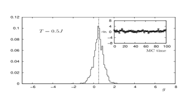
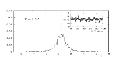
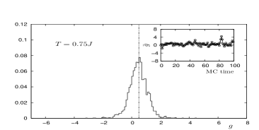
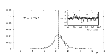
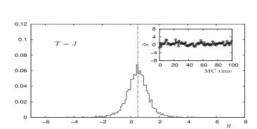
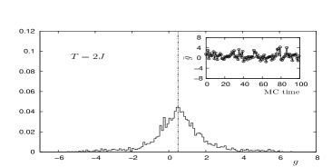
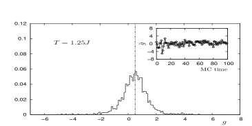
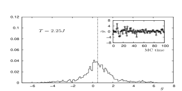
Figure 3: Probability distribution of the quantum-mechanical mean position of the conduction electron, $\bar{g}$, for different values of temperature, and $V=5\,J$. The probability distribution broadens with the growth of temperature. The insets show the value of $\bar{g}$ as a function of the MC time. At $T\geq 1.5\,J$ there is a large scatter of $\bar{g}$, which is the signature of the ferron depinning. Vertical dot-dashed line indicates the impurity position.

Using our approximate variational method, we can analyze the case of $V\rightarrow 0$. The plots for the correlation functions are very similar to those in of Fig. 2b. In this limit, we have $n=4$, so the ferron contains $8$ sites. The values of the corresponding characteristic temperatures are $T^{*}_{1}=2.97J$, $T^{*}_{2}=2.57J$, $T^{*}_{3}=1.31J$, and $T^{*}_{4}=0.14J$. Therefore, in our approach, we can describe both the ferron bound by impurity, and depinned from it. Some indication of this possible depinning at small values of $V$ could come from the presence of small ferromagnetic correlation corresponding to the fourth pair at high temperatures (see Fig. 2b).

To study the possible depinning in a more detailed way, we calculate the quantum-mechanical mean position $\bar{g}=Z^{-1}_{\text{el}}\sum\limits_{n}\sum\limits_{g}\langle\psi_{g}^{(n)}|\,g\,\psi_{g}^{(n)}\rangle\,e^{-\beta E_{n}}$ of the conduction electron for each MC time, where $Z_{\text{el}}=\sum\limits_{n}e^{-\beta E_{n}}$. Dependence of mean position $\bar{g}$ on MC time is shown in insets to Fig. 3. In this figure, we also show the histograms illustrating probability distribution of $\bar{g}$ in the temperature range $0<T<2.5J$, and for the set of parameters $V=5J,t=50J$. In the insets we can see that at temperatures $T\geq 1.5\,J$, there appears a large scatter in the values of mean position $\bar{g}$. Simultaneously, the probability distribution broadens. This means that an electron becomes depinned and can move far away from the impurity. Since the depinning temperature is, at least, lower than the temperatures $T^{*}_{1},T^{*}_{2}$ for the same values of $V$, and $t$, we can conclude that the ferron retains its magnetic structure after depinning. At sufficiently large values of $V$, the depinning of a ferron is not observed in the temperature range under study.

Figure 4: Standard deviation of $\bar{g}$, $\Delta g$, as a function of $T$. Different curves correspond to different impurity potentials: $V=0.1,\,1,\,5,$ and $100\,J$ (corresponding the first to the highest, and the last to the lowest curve, respectively).

In Fig. 4, we plot the standard deviation of the histograms of $\bar{g}$ as a function of temperature for several values of $V$. In all cases, the standard deviation has a maximum for some $T_{\text{max}}>J$. At relatively low temperatures, $\Delta g$ grows due to the increase in the thermal fluctuations of the ferron position. At higher temperatures, the ferromagnetic correlations forming the ferron gradually decay, and the electron undergoes a kind of Anderson localization in disordered spin background (the situation typical of the double exchange mechanism). Therefore, $\Delta g$ eventually decreases independently of the value of Coulomb potential $V$.

We can also find the depinning line using the variational method. Let us consider the ferron state bound to the impurity and the state at $V\to 0$. The latter case corresponds also to the free ferron located far from the impurity. The energy difference between bound and free ferron states then equals to $E(0,T_{dp})-E(V,T)$. The depinning temperature $T_{dp}$ can be estimated as:

$$E(0,T_{dp})-E(V,T_{dp})=T_{dp}\,,$$ (20)

where the mean energy of the system $E(V,T)$ is calculated by variational method using formula (III.1). Note that the depinning temperature calculated in such a way turns out to be in several times greater than its value estimated by Monte Carlo simulations, because in latter case we consider the states corresponding to the ferron located not far from the impurity.

In Fig. 5, we present the phase diagram of the chain in $V-T$ plane. The temperatures $T^{*}_{1},T^{*}_{2},\dots,T^{*}_{n}$ as a functions of the impurity potential are shown. We also plot the temperature $T^{*}_{AF}$ and the depinning line calculated by the variational method.

Figure 5: Phase diagram in the $V-T$ plane for a chain with a low density of bound ferrons. The value $t=50{J}$ is fixed. Solid line corresponds to $T^{*}_{1}$, that is, to the complete decay of the ferron. Dashed lines are the $T^{*}_{n/2}$ plots, depicting the decay of ferromagnetic correlations at the end pair of spins in the ferron. Horizontal line corresponds to the temperature $T^{*}_{AF}$. Dot-dashed line is the depinning line obtained by estimations described in the text. Above this line, ferrons are not bound by the impurities. Regions I and II above the “melting” line $T^{*}_{1}$ correspond to the free electron in the chain, and to the electron bound by the impurity in the absence of the ferron state.

V Conclusions

We show that the simple model of an antiferromagnetic chain with impurities captures the essential features of the phase separation in low-doped manganites. We find a set of temperatures characterizing the thermal evolution of the magnetic structure of such a chain. We demonstrate that the magnetic state of the chain is rather inhomogeneous and it can be described by a set of magnetic polarons. These magnetic polarons are rather stable objects existing at temperature even much higher than the Néel temperature of the undoped chain. With the growth of temperature, ferromagnetic correlations inside the ferron start to disappear in a step-wise way, up to some temperature $T^{*}_{1}\sim 0.1\,t-0.2\,t$, and then ferron state is no longer stable. The dynamics of ferrons depends on the magnitude of the electron-impurity coupling, $V$. At high values of $V$, ferron remains tightly bound by impurity, while at lower $V$, the ferron can be depinned from impurity at a characteristic temperature lower than $T^{*}_{1}$, and therefore retains its magnetic structure after depinning. These results can be summarized in the phase diagram in the $V-T$ plane presented in Fig. 5. We can see that in region below the rather flat curve $T^{*}_{1}$ versus $V$, there are the regions of stability of different kinds of ferrons, from $n=2$ to $8$ sites. In each such region, we show the dashed line corresponding to the melting of the last ferromagnetically correlated pair in the ferron. So, between the solid and each dashed line, we have the region where the ferron gradually decays. We also show the depinning line calculated by variational method as it was discussed at the end of the previous section. We see that there is a large region between the depinning line and $T^{*}_{1}$ where ferron is depinned. We have extended this depinning line above the $T^{*}_{1}$ curve to show the possible domains of existence of bare electron bound to the impurity and freely moving along the chain.

References

- (1) E. Dagotto, Nanoscale phase separation and colossal magnetoresistance: the physics of manganites and related compounds (Springer-Verlag, Berlin, 2003).
- (2) E. L. Nagaev, Pis’ma v ZhETF 6, 484 (1967) [JETP Lett. 6, 18 (1967)].
- (3) M. B. Salamon and M. Jaime, Rev. Mod. Phys. 73, 583 (2001).
- (4) M. A. Krivoglaz, Usp. Fiz. Nauk 106, 617 (1973) [Sov. Physics - Uspekhi 16, 856 (1974)].
- (5) M. Y. Kagan and K. I. Kugel, Usp. Fiz. Nauk 171, 577 (2001) [Physics - Uspekhi 44, 553 (2001)].
- (6) K. I. Kugel, A. L. Rakhmanov, A. O. Sboychakov, M. Y. Kagan, I. V. Brodsky, and A. V. Klaptsov, Zh. Eksp. Teor. Fiz. 125, 648 (2004) [JETP 98, 572 (2004)].
- (7) J. Castro, I. González, and D. Baldomir, Eur. Phys. J. B 39, 447 (2004).
- (8) I. González, J. Castro, D. Baldomir, A. O. Sboychakov, A. L. Rakhmanov, and K. I. Kugel, Phys. Rev. B69, 224409 (2004).
- (9) K. Binder, and D. W. Heermann, Monte Carlo simulation in statistical physics (Springer-Verlag, Berlin, 1997).
- (10) Yu. A. Izyumov and Yu. N. Skryabin, Usp. Fiz. Nauk 171, 121 (2001) [Physics - Uspekhi 44, 109 (2001)].
- (11) S. Yunoki, J. Hu, A. L. Malvezzi, A. Moreo, N. Furukawa, and E. Dagotto, Phys. Rev. Lett. 80, 845 (1998).
- (12) S. Pathak and S. Satpathy, Phys. Rev. B63, 214413 (2001).