Phase transitions in the Shastry-Sutherland lattice

Abstract

Two recently developed theoretical approaches are applied to the Shastry-Sutherland lattice, varying the ratio $J^{\prime}/J$ between the couplings on the square lattice and on the oblique bonds. A self-consistent perturbation, starting from either Ising or plaquette bond singlets, supports the existence of an intermediate phase between the dimer phase and the Ising phase. This existence is confirmed by the results of a renormalized excitonic method. This method, which satisfactorily reproduces the singlet triplet gap in the dimer phase, confirms the existence of a gapped phase in the interval $0.66<J^{\prime}/J<0.86$

I Introduction

Strongly correlated electron systems, and in particular those which can be treated as quantum magnets, are the subject of a continuous and intense attention from experimentalists and theoreticians. They frequently exbibit complex phase diagrams, and non-trivial low energy physics. Among the spin lattices those presenting spin frustrations both present unconventional phases and quantum phase transitions and represent a challenge for theoreticians. The quantum Monte Carlo methods, which may be considered as the most reliable treatment for non-frustrated 2-D or 3-D lattices, cannot be applied in these cases. Among the 2-D frustrated lattices one may quote the checkerboard, the Kagome and the triangular lattices, which have been the subject of numerous theoretical works. The $SrCu_{2}(BO_{3})_{2}$ lattice Ref1 is a famous two-dimensional anti-ferromagnetic system presenting a spin gap and free from long range order. The Copper atoms are of $d^{9}$ character and can be seen as $S=1/2$ spins. This lattice may be considered as a realization of the Shastry-Sutherland model Ref2 which can be schematized as a square lattice, with $J^{\prime}$ anti-ferromagnetic coupling between nearest neighbors, and diagonal anti-ferromagnetic interactions $J$ in one plaquette over two, as pictured in Fig. 1. This system is supposed to obey the corresponding Heisenberg Hamiltonian

$$H=J^{\prime}\sum_{[i,j]}\overrightarrow{S_{i}}\overrightarrow{S_{j}}+J\sum_{\langle i,j\rangle}\overrightarrow{S_{i}}\overrightarrow{S_{j}}$$ (1)

where the couples $[i,j]$ concern the bonds of the square lattice and ${\langle i,j\rangle}$ the connected pairs of next nearest neighbor atoms. The real material has been the subject of intense experimental studies, showing the existence of a spin gap,Ref3 an almost localized nature of the singlet triplet excitation,Ref4 and the existence of magnetization plateaux.Ref5 ; Ref6 The Shastry-Sutherland Hamiltonian has been widely studied by theoreticians (for review see S. Miyahara and K. Ueda Ref7 ), varying the $J^{\prime}/J$ ratio. For small values of $J^{\prime}/J$ the ground state is a product of singlets strictly localized on the oblique bonds. The real material would correspond to a ratio $J^{\prime}/J=0.635$, close to the critical value where this phase disappears. Oppositely when $J$ is small, the perturbed 2-D square lattice is gapless with long range order. Early studies based on exact diagonalizations,Ref8 Ising expansionRef9 or dimer expansions,Ref10 and real space renormalization group with effective interaction (RSRG-EI) Ref11 predict a simple transition between the Ising phase and the dimer phase for $J^{\prime}/J=0.696$. Other works have suggested the existence of an intermediate phase. From Schwinger boson mean field theory Ref12 this phase would be an helical ordered state, ranging between $J^{\prime}/J=0.6$ and 0.9 while a plaquette expansion Ref13 ; Ref14 predicts a plaquette singlet based phase for $0.677<J^{\prime}/J<0.86$, a result supported by other exact diagonalization results.Ref15 Weihong et al.Ref16 suggested that the intermediate phase between $J^{\prime}/J=0.69$ and 0.83 might be columnar rather than plaquette singlet.

The present paper employs two recently developed methods to study the phase diagram of this lattice. We first will consider the cohesive energy of the lattice, using a self consistent pertubation (SCP) Ref17 which may be seen as a modified coupled cluster expansion.Ref18 ; Ref19 ; Ref20 ; Ref21 The method starts from a reference function which can be the Ising spin distribution or a columnar product of bond singlets. It happens that the cohesive energy calculated from the latter reference function is the lower one for $0.66<J^{\prime}/J<0.86$, the lowest energy being obtained from the Ising reference for $J^{\prime}/J>0.86$. The calculated cohesive energies obtained by the RSRG-EI with $(3\times 3)$ sites square blocks or by the contractor renormalization (CORE)Ref22 with columnar blocks of $(2\times 6)$ sites agree with the values obtained from SCP and support the idea of an intermediate phase.

A second section concentrates on the calculation of the gap, using a renormalized excitonic method (REM), based on the scale-change ideas inspiring the renormalization group methods. The methods proceeds through the definition of blocks with even number of sites. The design of the relevant blocks is different for the dimer phase and for the other phases. The calculated gap for the dimer phase is in good agreement with that of previous theoretical study Ref13 ; Ref14 and compatible with experimental evidences.Ref7 Approaching the problem from columnar blocks one obtains a finite gap for $J^{\prime}/J<0.88$. This result confirms the existence of an intermediate phase.

II Calculation of the cohesive energy

If one defines $\lambda=J^{\prime}/(J^{\prime}+J)$ and take $J^{\prime}+J$ as the energy unit, the product of singlets on the oblique dimers ($J$ interactions) is an eigenfunction whatever $\lambda$, and its cohesive energy is $J^{\prime}+J=1$.

II.1 Self-consistent perturbation

We have used the recently proposed SCP method Ref17 to evaluate the cohesive energy of other phases. The method can be seen as a modified coupled cluster method.Ref18 ; Ref19 ; Ref20 ; Ref21 It starts from a reference function $\Phi_{0}$, supposed to be a relevant zero-order function for the considered phase. This function is highly localized. In practice $\Phi_{0}$ will be

• the Ising spin distribution on the square 2-D lattice,

• or a product of bond singlets in a columnar arrangement. On each of these bonds one may also define a local triplet state.

The action of $H$ on $\Phi_{0}$ generates a first generation of local excited function $\Phi_{i}$ ($\langle\Phi_{i}|H|\Phi_{0}\rangle\not=0$). In the so-called intermediate normalization convention

$$\Psi=\Phi_{0}+\sum_{i}C_{i}\Phi_{i}+\sum_{\alpha}C_{\alpha}\Phi_{\alpha},$$ (2)

where the vectors $\Phi_{\alpha}$ do not interact with $\Phi_{0}$ ($\langle\Phi_{\alpha}|H|\Phi_{0}\rangle=0$), the knowledge of the coefficients of the first generation $\Phi_{i}$’s is sufficient to fix the ground state energy

Figure 1: Genealogy of the wave function starting from Ising $\Phi_{0}$. $\Phi_{0}$ = reference function, $\Phi_{i}$ = first generation function, $\Phi_{\alpha}$, $\Phi_{\alpha^{\prime}}$, $\Phi_{\beta}$ types of non factorisable second generation functions.

$$E=\langle\Phi_{0}|H|\Phi_{0}\rangle+\sum_{i}C_{i}\langle\Phi_{0}|H|\Phi_{i}\rangle.$$ (3)

Starting from Ising $\Phi_{0}$, the vectors $\Phi_{i}$ are obtained by a spin exchange on any bond of the 2-D square lattice (Fig. 1). Starting from the product $\Phi^{\prime}_{0}$ of singlets on the $X$-directed bonds in a columnar arrangement (Fig. 2), the vectors $\Phi_{i}$ are excited singlet states produced as products of two triplets on interacting bonds. They are of four different types in a Shastry-Sutherland lattice, as pictured in Fig. 2.

The determination of the coefficients $C_{i}$ is governed by the corresponding eigenequation, adopting the compact notation $H_{ij}=\langle\Phi_{i}|H|\Phi_{j}\rangle$,

$$(H_{ii}-E)C_{i}+H_{i0}+\sum_{j}H_{ij}C_{j}+\sum_{\alpha\not\in S_{1}}H_{i\alpha}C_{\alpha}=0.$$ (4)

An estimation of the coefficients of the second generation functions $\Phi_{\alpha}$ (such that $H_{i\alpha}$)is only necessary for those which are obtained from $\Phi_{i}$ by operations in the strict neighborhood of the bonds involved in the process $T_{i}^{+}$ creating $\Phi_{i}$ from $\Phi_{0}$ ($\Phi_{i}=T_{i}^{+}\Phi_{0}$). The spin exchanges or excitations $T_{k}^{+}$ on remote bonds cancel, according to the linked cluster theorem, since in that case

$$C_{T_{k}^{+}|\Phi_{i}\rangle}=C_{k}C_{i}.$$ (5)

The number of second generation functions to be considered is therefore very limited. Their coefficient is estimated from the $C_{i}$’s according to perturbative arguments, with a systematic consideration of exclusion principle violating corrections of the energy denominators, which introduce infinite summations of diagrams and speed the convergence. Details of the method are given elsewhere.Ref17 The equations for the precise problem are given in the Appendix, the results appear in Fig. 3. One sees that

• the energy calculated from Ising $\Phi_{0}$ is the lowest one for large values of $J^{\prime}/J$. This energy curve cuts the energy of the localized dimer phase for $J^{\prime}/J=0.69$. This value compares quite well with other estimates,Ref8 ; Ref9 ; Ref10 ; Ref11 and in particular with that of a RSRG-EIRef11 with $(3\times 3)$ sites square blocks ($(J^{\prime}/J)_{c}=0.696$)

• however the energy calculated from the columnar arrangement of bond singlets on the 2-D square lattice happens to be lower than the preceding one for $J^{\prime}/J<0.859$. The corresponding energy is the lowest one for $0.661<J^{\prime}/J<0.859$. Hence these calculations support the suggestion of the existence of three phases, with an intermediate phase between the dimer phase and the Ising phase.

Figure 2: Genealogy of the wave function starting from columnar product of bond singlets empty ellipses. Dark ellipses represent local triplets. The figure pictures the 4 types of first generation singlet states. The non factorisable second generation functions are too numerous to be pictured.

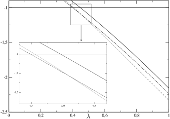
Figure 3: Cohesive energy (with the unit $(J+J^{\prime})$) as a function of the $\lambda$ parameter. The horizontal straight line concerns the dimer phase, - - - SCP expansion from columnar bond singlets $\Phi^{\prime}_{0}$, $\cdots$ SCP expansion from Ising $\Phi_{0}$, — SCP expansion from shifted bond singlets $\Phi^{\prime\prime}_{0}$.

However the fact that one finds two distinct values of the energy from two distinct reference functions within an approximate algorithm does not prove the existence of two phases. It is possible that at convergence the two wave operators, $\Omega$ from $\Phi_{0}$ and $\Omega^{\prime}$ from $\Phi^{\prime}_{0}$, lead to the same wave function

$$\Psi_{0}=\Omega\Phi_{0}=\Psi^{\prime}_{0}=\Omega^{\prime}\Phi^{\prime}_{0}.$$ (6)

As an argument in favor of two distinct phases we may mention that starting from an other function $\Phi^{\prime\prime}_{0}$, energetically degenerate with $\Phi^{\prime}_{0}$ ($\langle\Phi^{\prime\prime}_{0}|H|\Phi^{\prime\prime}_{0}\rangle=\langle\Phi^{\prime}_{0}|H|\Phi^{\prime}_{0}\rangle$), product of bond singlets on parallel bonds which do not belong to the same plaquette (see Fig. 4), the calculated energy always remains above that obtained from Ising $\Phi_{0}$, as seen in Fig. 3. It is not easy, at least from our SCP approach, to determine wether the intermediate phase is based on a columnar arrangement of bond singlets or is a plaquette phase. The second one keeps isotropic properties in the $X$ and $Y$ directions, while the former one breaks this symmetry. It is interesting to remark that our reference wave function $\Phi^{\prime}_{0}$ is strongly anisotropic, with a probability zero to find the parallel spins in the $X$-directed bonds of a plaquette and a probability 1/2 to find parallel spins in the $Y$-directed bonds. After consideration of the possible excitations, the probability to find parallel spins along the two $X$-directed bond of an empty plaquette becomes $87\%$ of the probability to find parallel spins on the $Y$-directed bonds of the same plaquette. The isotropy is almost restaured by the self-consistent evaluation of the excitation amplitudes. The result, obtained from a highly broken-symmetry reference function, pleads in favor of a plaquette phase.

Figure 4: Alternative reference function $\Phi^{\prime\prime}_{0}$.

II.2 Renormalization group methods

Renormalization group techniques have also been employed. A preceding work Ref11 had considered square 9 sites i.e., $(3\times 3)$ sites blocks, the ground state of which is an $S_{z}=\pm 1/2$ doublet, i.e., a quasi spin. The lattice of blocks is isomorphic to the Shastry-Sutherland lattice, with two types of effective interactions $J^{\prime(1)}$ and $J^{(1)}$ between the blocks, the amplitude of which can be obtained from the exact spectrum of the dimers of blocks, according to the effective Hamiltonian theory.Ref23 The ratio $J^{\prime(1)}/J^{(1)}$ is larger than $J^{\prime}/J$ for $J^{\prime}/J>0.696$. For $J^{\prime}/J=0.696$, $J^{\prime(1)}/J^{(1)}=J^{\prime}/J$, i.e., this value is a fixed point, for which the cohesive energy calculated by iterating the RSRG-EI procedure practically coincide with that of the dimer phase. The behaviour of the so-calculated cohesive energy of the Ising phase is plotted in Fig. 6. The intersection of the cohesive energy curves of the dimer phase and of the RSRG-EI estimate of the Ising phase occurs for $J^{\prime}/J=0.672$.Ref11 The method does not produce an intermediate phase, when it is applied to these isotropic square blocks.

If one uses 2n sites blocks, with a non degenerate singlet ground state $\psi_{A}^{0}$ of energy $E_{A}^{0}$, the ground state of the lattice is studied from the product of the ground state of the blocks $\Psi^{0}=\prod_{A}\psi_{A}^{0}$ according to the simplest version of the CORE method.Ref22 The knowledge of the ground state exact energy $E_{AB}^{0}$ of the $AB$ dimers enables one to define an effective interaction $v_{AB}$ between the blocksRef22 as

Table 1: Cohesive energy (with the unit $(J+J^{\prime})$) for intermediate values of the $J^{\prime}/J$ ratio.

$J^{\prime}/J$	SCP(Ising)	SCP(Plaquette)	$\mbox{CORE}^{\mbox{a}}$	$\mbox{RSRG-EI}^{\mbox{b}}$
0.65016	-0.97804	-0.99257	-0.99803	-0.98501
0.66667	-0.98987	-1.00355	-1.00787	-0.99609
0.69461	-1.00989	-1.02191	-1.02488	-1.01490
0.72413	-1.03026	-1.04034	-1.04251	-1.03362
0.81818	-1.09291	-1.09604	-1.09783	-1.09510
0.85185	-1.11419	-1.11475	-1.11720	-1.11790
1.0	-1.20061	-1.19028	-1.19478	-1.20920
(a) from $(2\times 6)$ sites columnar blocks
(b) from $(3\times 3)$ sites square blocks (cf. ref. 11).

Figure 5: (A) definition of the periodizable 12 sites blocks for the calculation of the excitation gap in the dimer phase, (B) definition of $(2\times 2n)$ sites columnar blocks for the calculation of the excitation gap in the plaquette phase, and application of the CORE method.

$$v_{AB}=E_{AB}^{0}-E_{A}^{0}-E_{B}^{0}$$ (7)

and the energy per block is

$$E_{A}=E_{A}^{0}+\frac{1}{2}\sum_{B}v_{AB}.$$ (8)

In the research of a tentative columnar phase, we have considered 12 $(2\times 6)$ sites columnar blocks built from three aligned plaquettes. Interestingly enough the calculated cohesive energy is the lowest one (cf Fig. 6) in the interval $0.656<J^{\prime}/J<0.845$ (RSRG-EI) or 0.901 (SCP). This result is in excellent agreement with our SCP result, and supports the existence of an intermediate plaquette phase. Table 1 reports the calculated values of the cohesive energy in the problematic domain of the $J^{\prime}/J$ ratio one sees the good agreement between the SCP from Ising and RSRG-EI on one hand and between the SCP from columnar arrangement of bond singlets and CORE with $(2\times 6)$ sites columnar blocks on the other hand.

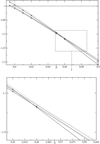
Figure 6: Evolution of the cohesive energy (with the unit $(J+J^{\prime})$) as a fonction of $\lambda=J^{\prime}/(J+J^{\prime})$. The horizontal line concerns the dimer phase, - - - SCP from columnar bond singlets $\Phi^{\prime}_{0}$, $\cdots$ SCP from Ising $\Phi_{0}$, —$\circ$— RSRG-EI from $(3\times 3)$ sites square blocks,Ref11 —$\Box$— CORE with $(2\times 6)$ sites columnar blocks. The lower part is a zoom in the region of crossing between the intermediate and Ising phases.

III Calculation of the singlet triplet gap

The study of the singlet triplet gap may bring additional informations. It has been performed according to an other renormalization group technique, the REM,Ref24 which starts from blocks $A$ with non degenerate ground state singlet $\psi^{0}_{A}$ and an excited triplet state $\psi_{A}^{\ast}$, and build the excited state from linear combinations of locally excited states, $\Psi_{A}^{\ast}=\psi_{A}^{\ast}\prod_{B}\psi_{B}^{0}$. The knowledge of the exact spectrum of the dimers of blocks makes possible the calculation of the effective interaction $v_{(A^{\ast})B}$ between an excited triplet and neighbor singlets and of an effective excitation-hopping integral $h_{AB}$ which couples $\psi_{A}^{\ast}\psi_{B}^{0}$ with $\psi^{0}_{A}\psi_{B}^{\ast}$.

We first have applied the method to the dimer phase. It is known that in this phase the triplet excitation on a given dimer bond can only propagate to a neighbor one through a 6th-order process involving a vortex of 4 dimers. A complete evaluation of the interaction leads to

This interaction remains small when $J^{\prime}$ increases, and the energy gap slowly deviates from $J$. A convenient design of 12 sites (6 dimers bonds) blocks involving two vortex have been pictured in Fig. 5(A). The gap calculated from the REM are reported in the left part of Fig. 7, together with those of a dimer expansion.Ref9 The excitation energy is tangent to the line $\Delta/J=1$ at the origin, as expected, but falls down rapidly near the phase transition. It vanishes for $J^{\prime}/J=0.7006$. For the $J^{\prime}/J=0.635$, i.e., the value proposed for the real material, our calculation gives $\Delta=0.32J$, which satisfactorily compares with the experimental value (30-35 K)Ref7 if one accepts the usually proposed value of $J$ (85 K).

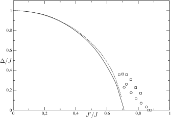
Figure 7: Dependence of the singlet-triplet gap on the $J^{\prime}/J$ ratio. — REM from 12-site blocks (Fig. 5(A)) for the dimer phase, - - - results of a dimer expansion,Ref9 $\circ$ extrapolated REM from columnar plaquette blocks (Fig. 5(B)), $\Box$ results of a plaquette expansion.Ref13 ; Ref14

For the columnar plaquette phase, blocks built from aligned plaquettes have been considered (Fig. 5(B)), together with an extrapolation on the block size.Ref24 The results appear in Fig. 7 together with those of a plaquette expansion.Ref13 ; Ref14 One sees that the system is gapped for $J^{\prime}/J<0.883$, and gapless beyond this value. The gap in this phase goes through a maximum for $J^{\prime}/J\simeq 0.73$, a result also obtained by Koga and Kawakami.Ref13 ; Ref14 Our results confirm the existence of an intermediate gapped phase.

IV Conclusion

The present work, employing essentially different methods based on either coupled cluster type expansions or renormalization group techniques, present consistent results confirming the existence of an intermediate phase in the Shastry-Sutherland lattice, and its plaquette or columnar nature. The results regarding the location of the phase transitions are gathered in Table 2. While the phase transition between the dimer and the Ising phases would occur at $J^{\prime}/J$ between 0.67 and 0.70, the intermediate phase is the lowest one from $J^{\prime}/J=0.656$ (CORE 12 sites) - 0.661 (SCP) to $J^{\prime}/J=0.859$ (SCP) - 0.901 (CORE/SCP). Obtained from new methods, these results agree with those of refs. 13-16 and reduce the remaining uncertainties concerning the existence, domain and nature of the intermediate phase in the Shastry-Sutherland lattice.

Table 2: Critical values of the $J/J^{\prime}$ ratio, based on cohesive energy (Coh) or gap calculations (Gap).

	Criterion	Methods	$J^{\prime}/J$
	Coh	$\mbox{dimer}^{\mbox{a}}/\mbox{SCP}^{\mbox{b}}$	0.690
Dimer/Ising	Coh	$\mbox{dimer}^{\mbox{a}}/\mbox{RSRG-EI}^{\mbox{c}}$	0.672
	Gap	$\mbox{REM}^{\mbox{d}}$	0.701
	Coh	$\mbox{dimer}^{\mbox{a}}/\mbox{SCP}^{\mbox{e}}$	0.661
Dimer/Interm.	Coh	$\mbox{dimer}^{\mbox{a}}/\mbox{CORE}^{\mbox{f}}$	0.656
	Coh	$\mbox{SCP}^{\mbox{e}}/\mbox{SCP}^{\mbox{b}}$	0.859
	Coh	$\mbox{CORE}^{\mbox{f}}/\mbox{SCP}^{\mbox{b}}$	0.901
Interm./Ising	Coh	$\mbox{SCP}^{\mbox{e}}/\mbox{RSRG-EI}^{\mbox{c}}$	0.826
	Coh	$\mbox{CORE}^{\mbox{f}}/\mbox{RSRG-EI}^{\mbox{c}}$	0.845
	Gap	$\mbox{REM}^{\mbox{g}}$	0.883
(a) exact energy
(b) from Ising $\Phi_{0}$
(c) from $(3\times 3)$ sites square blocks (cf. ref. 11)
(d) gap vanishing of the dimer phase, 12-site blocks
(Fig. 5(A))
(e) from columnar bond singlets $\Phi^{\prime}_{0}$
(f) from $(2\times 6)$ sites columnar blocks
(g) gap vanishing of the Intermediate phase,
extrapolations from columnar blocks.

Appendix A

SCP equations for the Shastry-Sutherland lattice
(1) Equation from Ising function. There is a unique type of spin exchange, and a single coefficient $C$.

$$\big{[}6J^{\prime}-2J-7J^{\prime}C\big{]}C+J^{\prime}+JC+J^{\prime}\Bigg{[}2\Bigg{(}\frac{12J^{\prime}-4J-14J^{\prime}C}{8J^{\prime}-4J-12J^{\prime}C}\Bigg{)}-1\Bigg{]}C^{2}+J^{\prime}\Bigg{[}2\Bigg{(}\frac{12J^{\prime}-4J-14J^{\prime}C}{8J^{\prime}-2J-12J^{\prime}C}\Bigg{)}-1\Bigg{]}C^{2}$$

$$+4J^{\prime}\Bigg{[}\frac{12J^{\prime}-4J-14J^{\prime}C}{10J^{\prime}-2J-13J^{\prime}C}-1\Bigg{]}C^{2}+10J^{\prime}\Bigg{[}\frac{12J^{\prime}-4J-14J^{\prime}C}{10J^{\prime}-4J-13J^{\prime}C}-1\Bigg{]}C^{2}+2J^{\prime}\Bigg{[}\frac{12J^{\prime}-4J-14J^{\prime}C}{12J^{\prime}-2J-14J^{\prime}C}-1\Bigg{]}C^{2}$$

$$-\frac{J^{2}C}{8J^{\prime}-2J-8J^{\prime}C}=0,$$ (9)

$$E_{coh}=-2J^{\prime}(1-C).$$ (10)

(2) Equations from bond singlets functions. There are four types of double excitations, as pictured in Fig. 2. Using the notations

$$\langle\Phi^{\prime}_{0}|H|\Phi^{\prime}_{ii^{\prime}}\rangle=h_{1}=\frac{\sqrt{3}\big{[}2J^{\prime}-J\big{]}}{2},\ \langle\Phi^{\prime}_{0}|H|\Phi^{\prime}_{ii^{\prime\prime}}\rangle=h_{2}=\sqrt{3}J^{\prime},\ \langle\Phi^{\prime}_{0}|H|\Phi^{\prime}_{ij}\rangle=h_{3}=\frac{\sqrt{3}J^{\prime}}{2},\ \langle\Phi^{\prime}_{0}|H|\Phi^{\prime}_{ih^{\prime}}\rangle=h_{4}=\frac{\sqrt{3}J}{2}$$

the four coupled polynomial equations are

$$\big{[}2J^{\prime}-J-\big{(}h_{1}C_{1}+2h_{2}C_{2}+4h_{3}C_{3}+2h_{4}C_{4}\big{)}\big{]}C_{1}+h_{1}+\frac{2h_{1}C_{3}^{2}}{3}$$

$$-\frac{1}{3}\Bigg{[}\frac{2h_{2}\big{(}h_{2}C_{1}+h_{1}C_{2}\big{)}+4h_{3}\big{(}2h_{3}C_{1}+2h_{1}C_{3}\big{)}+2h_{4}\big{(}h_{4}C_{1}+h_{1}C_{4}\big{)}}{4J^{\prime}-\big{(}2h_{1}C_{1}+2h_{2}C_{2}+4h_{3}C_{3}+2h_{4}C_{4}\big{)}}\Bigg{]}=0,$$ (11)

$$\big{[}2J^{\prime}-\big{(}2h_{1}C_{1}+h_{2}C_{2}+4h_{3}C_{3}+2h_{4}C_{4}\big{)}\big{]}C_{2}+h_{2}-\frac{2\big{[}h_{4}C_{3}+h_{3}C_{4}\big{]}}{\sqrt{3}}+\frac{2h_{2}C_{3}^{2}}{3}$$

$$-\frac{1}{3}\Bigg{[}\frac{2h_{1}\big{(}h_{1}C_{2}+h_{2}C_{1}\big{)}+2h_{3}\big{(}2h_{3}C_{2}+2h_{2}C_{3}\big{)}}{4J^{\prime}-\big{(}2h_{1}C_{1}+2h_{2}C_{2}+4h_{3}C_{3}+2h_{4}C_{4}\big{)}}\Bigg{]}=0,$$ (12)

$$\big{[}3J^{\prime}-\big{(}2h_{1}C_{1}+2h_{2}C_{2}+3h_{3}C_{3}+2h_{4}C_{4}\big{)}\big{]}C_{3}+h_{3}-\frac{h_{2}C_{4}+h_{4}C_{2}}{\sqrt{3}}+\frac{h_{3}\big{[}C_{1}^{2}+C_{2}^{2}+C_{4}^{2}\big{]}}{3}$$

$$-\frac{1}{3}\Bigg{[}\frac{2h_{1}\big{(}2h_{1}C_{3}+2h_{3}C_{1}\big{)}+h_{2}\big{(}2h_{2}C_{3}+2h_{3}C_{2}\big{)}+4h_{3}^{2}C_{3}+h_{4}\big{(}2h_{4}C_{3}+2h_{3}C_{4}\big{)}}{4J^{\prime}-\big{(}2h_{1}C_{1}+2h_{2}C_{2}+4h_{3}C_{3}+2h_{4}C_{4}\big{)}}\Bigg{]}=0,$$ (13)

$$\big{[}4J^{\prime}-J-\big{(}2h_{1}C_{1}+2h_{2}C_{2}+4h_{3}C_{3}+h_{4}C_{4}\big{)}\big{]}C_{4}+h_{4}-\frac{2\big{[}h_{2}C_{3}+h_{3}C_{2}\big{]}}{\sqrt{3}}+\frac{2h_{4}C_{3}^{2}}{3}$$

$$-\frac{1}{3}\Bigg{[}\frac{2h_{1}\big{(}h_{1}C_{4}+h_{4}C_{1}\big{)}+2h_{3}\big{(}2h_{3}C_{4}+2h_{4}C_{3}\big{)}}{4J^{\prime}-\big{(}2h_{1}C_{1}+2h_{2}C_{2}+4h_{3}C_{3}+2h_{4}C_{4}\big{)}}\Bigg{]}=0,$$ (14)

$$E_{coh}=\frac{\big{[}-(7J^{\prime}+J)+h_{1}C_{1}+h_{2}C_{2}+2h_{3}C_{3}+h_{4}C_{4}\big{]}}{4}.$$ (15)

References

• (1) R. W. Smith and D. A. Keszler, J. Solid State Chem. 93, 430 (1991).
• (2) B. S. Shastry and B. Sutherland, Physica (Amsterdam) 108B, 1069 (1981).
• (3) H. Kageyama et al., J. Phys. Soc. Jpn. 68, 1821 (1999).
• (4) H. Kageyama et al., Phys. Rev. Lett. 84, 5876 (2000).
• (5) H. Kageyama et al., Phys. Rev. Lett. 82, 3168 (1999).
• (6) K. Onizuka et al., J. Phys. Soc. Jpn. 69, 1016 (2000).
• (7) S. Miyahara and K. Ueda, J. Phys.: Condens. Matter. 15, R327 (2003).
• (8) S. Miyahara and K. Ueda, Phys. Rev. Lett. 82, 3701 (1999).
• (9) W. Zheng, C. J. Hamer, and J. Oitmaa, Phys. Rev. B 60, 6608 (1999).
• (10) E. MΓΌller-Hartmann, R.R.P. Singh, C. Knetter, and G.S. Uhrig, Phys. Rev. Lett. 84, 1808 (2000).
• (11) M. Al Hajj, N. GuihΓ©ry, J.-P. Malrieu, and B. Bocquillon, Eur. Phys. J. B 41, 11 (2004).
• (12) M. Albrecht and F. Mila, EuroPhys. Lett. 34, 145 (1996).
• (13) A. Koga and N. Kawakami, Phys. Rev. Lett. 84, 4461 (2000).
• (14) Y. Takushima, A. Koga, and N. Kawakami, J. Phys. Soc. Jpn. 70, 1369 (2000).
• (15) A. LΓ€uchli, S. Wessel, and M. Sigrist, Phys. Rev. B 66, 014401 (2002).
• (16) W. Zheng, J. Oitmaa, and C. J. Hamer, Phys. Rev. B 65, 014408 (2002).
• (17) M. Al Hajj and J.-P. Malrieu, Phys. Rev. B 70, 184441 (2004).
• (18) F. Coester and H. KΓΌmmel, Nucl. Phys. 17, 477 (1960).
• (19) J. CΜ†izΜ†ek, J. Chem. Phys. 45, 4256 (1966).
• (20) J. CΜ†izΜ†ek and J. Paldus, Physica Scripta 21, 251 (1980).
• (21) G. D. Purvis and R. J. Bartlett, J. Chem. Phys. 68, 2114 (1978).
• (22) C. J. Morningstar and M. Weinstein, Phys. Rev. D 54, 4131 (1996).
• (23) C. Bloch, Nucl. Phys. 6, 329 (1958).
• (24) M. Al Hajj, J.-P. Malrieu, and N. GuihΓ©ry, cond-mat/0411541.