Weak antilocalization in high-mobility two-dimensional systems

Abstract

Theory of weak antilocalization is developed for high-mobility two-dimensional systems. Spin-orbit interaction of Rashba and Dresselhaus types is taken into account. Anomalous magnetoresistance is calculated in the whole range of classically weak magnetic fields and for arbitrary strength of spin-orbit splitting. Obtained expressions are valid for both ballistic and diffusive regimes of weak localization. Proposed theory includes both backscattering and nonbackscattering contributions to the conductivity. It is shown that magnetic field dependence of conductivity in high-mobility structures is not described by earlier theories.

I Introduction

Anomalous magnetoresistance caused by weak localization is a powerful tool for extracting kinetic and band-structure parameters of three-dimensional (3D) and 2D systems.AA Theoretical expression for magnetoconductivity valid in the whole range of classically weak magnetic fields taking into account all interference processes has been first derived in Ref.Zyuzin, . In the absence of spin-orbit interaction the sign of the magnetoresistance is negative.

However the anomalous magnetoresistance is an alternating function in 2D semiconductor systems. In particular, in low fields it is positive and cannot be described by the theory Ref.Zyuzin, . The reason for positive magnetoresistance is a spin-orbit interaction. In semiconductor heterostructures it is described by the following Hamiltonian

$$H(\bm{k})=\hbar\>\bm{\sigma}\cdot\bm{\Omega}(\bm{k}),$$ (1)

where $\bm{k}$ is the electron wave vector, $\bm{\sigma}$ is the vector of Pauli matrices, and $\bm{\Omega}$ is an odd function of $\bm{k}$. The spin splitting due to spin-orbit interaction Eq. (1) equals to $2\hbar\Omega({\bm{k}})$.

In the presence of spin splitting, weak magnetic field decreases conductivity. Therefore the effect in such systems is called weak antilocalization. Theory of magnetoresistance in systems with spin-orbit interaction Eq.(1) was developed in Ref.ILP, . However the obtained expressions are valid only for i)weak spin-orbit interaction and ii)very low magnetic fields. The first assumption means that $\Omega\tau\ll 1$, where $\tau$ is the scattering time. The second condition reads as $l_{B}\gg l$, where $l_{B}=\sqrt{\hbar/eB}$ is the magnetic length, and $l$ is the mean free path. This so-called “diffusion” regime takes place in fields $B\ll B_{tr}$, where

$$B_{tr}={\hbar\over 2el^{2}}$$

is the “transport” field.

In high-mobility structures both these conditions fail. Due to long scattering times the product $\Omega\tau$ can be even larger than unity.Harley ; WAL&SIA ; WAL_Yulik_PRL ; Hamburg Besides, the transport field is often less than 1 mT, WAL&SIA ; WAL_Yulik_PRL ; Stud that is too small range of magnetic fields. This means that particle motion is rather ballistic than diffusive. Therefore fitting experimental data by the theories Refs.Zyuzin, ; ILP, is not always successful.Stud

An attempt to derive the field dependence of anomalous magnetoresistance for high-mobility structures has been performed in Ref.WAL_Yulik_PRL, . However the developed theory is correct only for high fields $B/B_{tr}\gg(\Omega\tau)^{2}$ and ignores some contributions to the conductivity.

The aim of the present work is to develop the weak-antilocalization theory for systems with strong spin-orbit interaction valid for both ballistic and diffusion regimes. The magnetic field dependence of the conductivity is calculated for arbitrary values of $B/B_{tr}$ and $\Omega\tau$, opening a possibility to describe anomalous magnetoresistance experiments and to extract spin-splitting and kinetic parameters of high-mobility 2D systems.

II Theory

There are two $\bm{k}$-linear contributions to the spin-orbit interaction Hamiltonian Eq. (1) in 2D semiconductor systems: the Rashba term $\bm{\Omega}_{R}$ and the Dresselhaus term $\bm{\Omega}_{D}$. In heterostructures grown along the direction $z\parallel[001]$ both vectors $\bm{\Omega}_{R,D}$ lie in the 2D plane and have the following form

$$\bm{\Omega}_{R}=\Omega_{R}\,(\sin{\chi},-\cos{\chi}),\>\>\>\bm{\Omega}_{D}=\Omega_{D}\,(\cos{\chi},-\sin{\chi}).$$ (2)

Here the axes are chosen as $x\parallel[100]$, $y\parallel[010]$, and $\tan{\chi}=k_{y}/k_{x}$. The anomalous magnetoresistance is the same if one takes into account the Rashba or the Dresselhaus contribution. Therefore we consider below only one term in $\bm{\Omega}$ with an isotropic spin splitting $2\hbar\Omega\sim k$.

Retarded and advanced Green functions of a system with the spin-orbit interaction Eqs. (1), (2) are $2\times 2$ matrices in the spin space. In the Landau gauge under scattering from a short-range potential, they are given bySTNS

$$G^{R,A}(\bm{r},\bm{r}^{\prime})=\sum_{Nqs}{\Psi_{Nqs}(\bm{r})\Psi_{Nqs}^{\dagger}(\bm{r}^{\prime})\over E_{\rm F}-E_{Ns}\pm{\rm i}\hbar/2\tau\pm{\rm i}\hbar/2\tau_{\phi}}.$$ (3)

Here $E_{\rm F}$ is the Fermi energy, $N$ is a number of the Landau level, $q$ is the wave vector in the 2D plane, $\tau_{\phi}$ is a phase relaxation time, $s=\pm$ enumerates two spin states, $E_{Ns}$ is the electron energy, and two-component spinors $\Psi_{Nqs}$ are the electron wave functions in the presence of magnetic field and the spin-orbit interaction Eq. (1). For Rashba spin-splitting, $\Psi_{Nqs}$ is a superposition of the electron states $|N,q,\uparrow\rangle$ and $|N+1,q,\downarrow\rangle$,Rashba i.e. with the same $N+s_{z}$, where $s_{z}$ is the spin projection onto the growth axis. The Dresselhaus spin-orbit interaction mixes the states with equal $N-s_{z}$.

In low magnetic fields

$$\omega_{c}\ll\Omega,\>\tau^{-1}\ll E_{\rm F}/\hbar,$$ (4)

where $\omega_{c}$ is the cyclotron frequency, one can show that both magnetic field and spin-orbit interaction result in an appearance of phases in the Green functions

$$G^{R,A}(\bm{r},\bm{r}^{\prime})=G^{R,A}_{0}(R)\>\exp{\left[{\rm i}\varphi(\bm{r},\bm{r}^{\prime})-{\rm i}\tau\bm{\sigma}\cdot\bm{\omega}(\bm{R})\right]}.$$ (5)

Here $\bm{R}\equiv(X,Y)=\bm{r}-\bm{r}^{\prime}$, $G^{R,A}_{0}(R)$ are the Green functions at $B=0$ and $\Omega=0$, and $\varphi(\bm{r},\bm{r}^{\prime})=(x+x^{\prime})(y^{\prime}-y)/2l_{B}^{2}$. The vectors $\bm{\omega}(\bm{R})$ are determined by the symmetry of a spin-orbit interactionLK

$$\bm{\omega}_{R}(\bm{R})={\Omega_{R}\over l}(Y,-X),\hskip 19.91684pt\bm{\omega}_{D}(\bm{R})={\Omega_{D}\over l}(X,-Y).$$ (6)

The weak-localization correction to conductivity is determined by interference of paths passing by a scattering particle in opposite directions. The amplitude of this interference, Cooperon, depends on four spin indices: ${\cal C}_{\alpha\beta,\gamma\delta}(\bm{r},\bm{r}^{\prime})$. Here $\alpha$ and $\beta$ ($\gamma$ and $\delta$) are the spin states of a particle before and after passing the path between the points $\bm{r}$ and $\bm{r}^{\prime}$ in the 2D plane forward (backward). The Cooperon satisfies the matrix equation

$${\cal C}(\bm{r},\bm{r}^{\prime})={\hbar^{3}\over m\tau}P(\bm{r},\bm{r}^{\prime})+\int d\bm{r}_{1}P(\bm{r},\bm{r}_{1}){\cal C}(\bm{r}_{1},\bm{r}^{\prime}),$$ (7)

where $m$ is the electron effective mass and

$$P_{\alpha\gamma,\beta\delta}(\bm{r},\bm{r}^{\prime})={\hbar^{3}\over m\tau}G^{R}_{\alpha\beta}(\bm{r},\bm{r}^{\prime})G^{A}_{\gamma\delta}(\bm{r},\bm{r}^{\prime})$$

is the probability for an electron to propagate from $\bm{r}$ to $\bm{r}^{\prime}$ forward and backward.WAL_Yulik_PRL It follows from Eq. (5) that

$$P(\bm{r},\bm{r}^{\prime})=P_{0}(R)\>\exp{\left[2{\rm i}\varphi(\bm{r},\bm{r}^{\prime})-2{\rm i}\tau\bm{S}\cdot\bm{\omega}(\bm{R})\right]},$$ (8)

where $\bm{S}_{\alpha\gamma,\beta\delta}=(\bm{\sigma}_{\alpha\beta}+\bm{\sigma}_{\gamma\delta})/2$ is an operator of the total angular momentum of two interfering particles, and

$$P_{0}(R)={\exp{(-R/\tilde{l})}\over 2\pi Rl}$$

is the value of $P$ in the absence of a magnetic field and a spin-orbit interaction. Here the effective scattering length $\tilde{l}=l/(1+\tau/\tau_{\phi})$.

In order to find the Cooperon, we expand the matrix $P$ into the series over wave functions of a spinless particle with the charge $2e$ in a magnetic field

$$P(\bm{r},\bm{r}^{\prime})=\sum_{NN^{\prime}q}P(N,N^{\prime})\>\Phi_{Nq}(\bm{r})\Phi_{N^{\prime}q}^{*}(\bm{r}^{\prime}).$$ (9)

The expansion coefficients are given by

$$P(N,N^{\prime})=\int d\bm{r}\>P_{0}(r)\exp{[-2{\rm i}\tau\bm{S}\cdot\bm{\omega}(\bm{r})]}F_{NN^{\prime}}(\bm{r}),$$

where

$$F_{NN^{\prime}}(\bm{r})=e^{-t^{2}/2}\>L_{N}^{N^{\prime}-N}(t^{2})\>(-te^{{\rm i}\phi})^{N^{\prime}-N}\>\sqrt{N!\over N^{\prime}!}.$$

Here $t=r/l_{B}$, $\tan\phi=y/x$, and $L_{N}^{M}$ are the associated Laguerre polynomials. At $\Omega=0$, $P(N,N^{\prime})\sim\delta_{NN^{\prime}}$. Finite spin splitting leads to nonzero values of $P(N,N^{\prime})$ with $|N-N^{\prime}|\leq 2$.

Expanding the Cooperon ${m\tau\over\hbar^{3}}{\cal C}(\bm{r},\bm{r}^{\prime})$ in series (9) as well, we obtain the following infinite system of linear equations for its expansion coefficients

$${\cal C}(N,N^{\prime})=P(N,N^{\prime})+\sum_{N_{1}}P(N,N_{1}){\cal C}(N_{1},N^{\prime}).$$ (10)

In order to solve this system, we turn to the representation of total angular momentum of two particles $\bm{S}$: $\alpha\gamma\to Sm_{s}$, where $S=0,1$ is the absolute value of $\bm{S}$, and $m_{s}$ is its projection onto the $z$ axis ($|m_{s}|\leq S$). The pair of particles with $S=0$ is in the singlet state while $S=1$ corresponds to the triplet one.

Spin-orbit interaction Eq. (1) with only one contribution Eq. (2) remains the energy spectrum isotropic. Therefore the particles being in the singlet and triplet states do not interfere, and there are two uncoupled Cooperons corresponding to the triplet and singlet, ${\cal C}_{T}$ and ${\cal C}_{S}$.

The singlet part is independent of the spin splitting and can be found from Eq. (10) as for $\Omega=0$:

$${\cal C}_{S}(N,N^{\prime})={P_{N}\over 1-P_{N}}\delta_{NN^{\prime}},$$ (11)

where

$$P_{N}={l_{B}\over l}\int\limits_{0}^{\infty}dx\exp{\left(-x{l_{B}\over\tilde{l}}-{x^{2}\over 2}\right)}L_{N}(x^{2}).$$

The triplet part ${\cal C}_{T}(N,N^{\prime})$ satisfies Eq. (10) with an infinite matrix $P_{T}(N,N^{\prime})$. ${\cal C}_{T}$ and $P_{T}$ are matrices with respect to both $N,N^{\prime}$ and $m_{s},m_{s}^{\prime}=1,0,-1$. It is crucial that $P_{T}$ can be decomposed into $3\times 3$ blocks. For Rashba spin-orbit interaction, it takes place in the basis of the states $|N,m_{s}\rangle$ with equal $N+m_{s}$: $|N-2,1\rangle$, $|N-1,0\rangle$, $|N,-1\rangle$, while for Dresselhaus term this takes place for the states with the same $N-m_{s}$. In both cases the blocks in $P_{T}$ can be obtained by a unitary transformation from the following matrix

$$A_{N}=\left(\begin{array}[]{ccc}P_{N-2}-S_{N-2}^{(0)}&R_{N-2}^{(1)}&S_{N-2}^{(2)}\\ R_{N-2}^{(1)}&P_{N-1}-2S_{N-1}^{(0)}&R_{N-1}^{(1)}\\ S_{N-2}^{(2)}&R_{N-1}^{(1)}&P_{N}-S_{N}^{(0)}\\ \end{array}\right).$$

Here

$$S_{N}^{(m)}={l_{B}\over l}\sqrt{N!\over(N+m)!}$$

$$\times \int\limits_{0}^{\infty}dx\exp{\left(-x{l_{B}\over l}-{x^{2}\over 2}\right)}x^{m}L_{N}^{m}(x^{2})\sin^{2}\left(\Omega\tau{l_{B}\over l}x\right),$$

$$R_{N}^{(m)}={l_{B}\over l\sqrt{2}}\sqrt{N!\over(N+m)!}$$

$$\times \int\limits_{0}^{\infty}dx\exp{\left(-x{l_{B}\over l}-{x^{2}\over 2}\right)}x^{m}L_{N}^{m}(x^{2})\sin\left(2\Omega\tau{l_{B}\over l}x\right).$$

The triplet part of the Cooperon is expressed via the matrix (II) as follows: it consists of the blocks ${\cal C}_{T}(N)$ given by

$${\cal C}_{T}(N)=A_{N}(I-A_{N})^{-1},$$ (12)

where $I$ is a $3\times 3$ unit matrix.

The conductivity correction due to weak antilocalization is given by a sum of two termsZyuzin

$$\sigma(B)=\sigma_{a}+\sigma_{b},$$

where $\sigma_{a}$ and $\sigma_{b}$ can be interpreted as backscattering and nonbackscattering interference corrections to conductivity.DKG They are given by

$$\sigma_{a}={\hbar\over 4\pi}\int d{\bm{r}}\int d{\bm{r}}^{\prime}\sum_{\alpha\beta\gamma\delta}\widetilde{\cal C}_{\alpha\gamma,\beta\delta}({\bm{r}},{\bm{r}}^{\prime})$$ (13)

$$\times{\bm{J}}_{\delta\alpha}({\bm{r}}^{\prime},{\bm{r}})\cdot{\bm{J}}_{\beta\gamma}({\bm{r}}^{\prime},{\bm{r}}),$$

$$\sigma_{b}={\hbar^{4}\over 2\pi m\tau}\int d{\bm{r}}\int d{\bm{r}}^{\prime}\int d{\bm{r}}^{\prime\prime}\sum_{\alpha\beta\gamma\delta\mu\nu}{\cal C}_{\alpha\gamma,\beta\delta}({\bm{r}},{\bm{r}}^{\prime})$$ (14)

$$\times\Biggl{[}J^{x}_{\delta\mu}({\bm{r}}^{\prime},{\bm{r}}^{\prime\prime})J^{x}_{\nu\gamma}({\bm{r}}^{\prime\prime},{\bm{r}})G^{A}_{\beta\nu}({\bm{r}}^{\prime},{\bm{r}}^{\prime\prime})G^{A}_{\mu\alpha}({\bm{r}}^{\prime\prime},{\bm{r}})$$

$$+J^{x}_{\beta\nu}({\bm{r}}^{\prime},{\bm{r}}^{\prime\prime})J^{x}_{\mu\alpha}({\bm{r}}^{\prime\prime},{\bm{r}})G^{R}_{\delta\mu}({\bm{r}}^{\prime},{\bm{r}}^{\prime\prime})G^{R}_{\nu\gamma}({\bm{r}}^{\prime\prime},{\bm{r}})\Biggr{]}.$$

Appearance of the modified Cooperon $\widetilde{\cal C}={\cal C}-{\hbar^{3}\over m\tau}P$ follows from that only three and more scattering events contribute to the magnetoconductivity.

The current vertex is defined as

$${\bm{J}}({\bm{r}},{\bm{r}}^{\prime})=e\int d{\bm{r}}_{1}G^{R}({\bm{r}},{\bm{r}}_{1}){\bm{v}}({\bm{r}}_{1})G^{A}({\bm{r}}_{1},{\bm{r}}^{\prime}),$$

where $\bm{v}$ is the velocity operator in a magnetic field. Substituting here the Green functions in the form Eq. (3), one can show for low magnetic fields Eq. (4) that

$$J^{\pm}_{\alpha\beta}({\bm{r}},{\bm{r}}^{\prime})={{\rm i}el\over\hbar}\>e^{\pm{\rm i}\theta}\left[G^{R}_{\alpha\beta}({\bm{r}},{\bm{r}}^{\prime})+G^{A}_{\alpha\beta}({\bm{r}},{\bm{r}}^{\prime})\right],$$ (15)

where $J^{\pm}=J^{x}\pm{\rm i}J^{y}$, and $\theta$ is an angle between ${\bm{r}}$ and ${\bm{r}}^{\prime}$.

Omitting the rapidly oscillating products $G^{R}G^{R}$ and $G^{A}G^{A}$ and expanding the terms

$$K({\bm{r}},{\bm{r}}^{\prime})={\rm i}\cos{\theta}\>P({\bm{r}},{\bm{r}}^{\prime})$$

in series Eq. (9), we get from Eqs. (13)-(15) the final expressions for the conductivity corrections

$$\sigma_{a}=-{e^{2}\over 2\pi^{2}\hbar}\left({l\over l_{B}}\right)^{2}\sum_{N=0}^{\infty}\Biggl{\{}{\rm Tr}\left[A_{N}^{3}(I-A_{N})^{-1}\right]-{P_{N}^{3}\over 1-P_{N}}\Biggr{\}},$$ (16)

$$\sigma_{b}={e^{2}\over 4\pi^{2}\hbar}\left({l\over l_{B}}\right)^{2}\sum_{N=0}^{\infty}\Biggl{\{}{\rm Tr}\left[K_{N}\widetilde{K}_{N}A_{N}(I-A_{N})^{-1}\right]$$ (17)

$$+{\rm Tr}\left[\widetilde{K}_{N}K_{N}A_{N+1}(I-A_{N+1})^{-1}\right]$$

$$-Q_{N}^{2}\left({P_{N}\over 1-P_{N}}+{P_{N+1}\over 1-P_{N+1}}\right)\Biggr{\}}.$$

The terms with matrices here are the triplet contributions which is seen to be of opposite sign in comparison to the singlet ones. The matrices $K_{N}$ and $\widetilde{K}_{N}$ appearing in the expansion of the function $K({\bm{r}},{\bm{r}}^{\prime})$ are given by

$$K_{N}=\left(\begin{array}[]{ccc}Q_{N-2}-S_{N-2}^{(1)}&R_{N-2}^{(2)}&S_{N-2}^{(3)}\\ -R_{N-1}^{(0)}&Q_{N-1}-2S_{N-1}^{(1)}&R_{N-1}^{(2)}\\ -S_{N-1}^{(1)}&-R_{N}^{(0)}&Q_{N}-S_{N}^{(1)}\\ \end{array}\right),$$

$$\widetilde{K}_{N}=\left(\begin{array}[]{ccc}Q_{N-2}-S_{N-2}^{(1)}&-R_{N-1}^{(0)}&S_{N-1}^{(1)}\\ -R_{N-2}^{(2)}&Q_{N-1}-2S_{N-1}^{(1)}&-R_{N}^{(0)}\\ S_{N-2}^{(3)}&-R_{N-1}^{(2)}&Q_{N}-S_{N}^{(1)}\\ \end{array}\right),$$

where

$$Q_{N} ={1\over\sqrt{N+1}}{l_{B}\over l}$$

$$\times \int\limits_{0}^{\infty}dx\exp{\left(-x{l_{B}\over l}-{x^{2}\over 2}\right)}xL_{N}^{1}(x^{2}).$$

Note that the values with negative indices appearing in Eqs. (II), (II), and (II) at $N=0,1$ should be replaced by zeros.

Eqs. (16) and (17) yield the weak-antilocalization correction to the conductivity in the whole range of classically-weak magnetic fields and for arbitrary values of $\Omega\tau$.

III Limiting cases

In the limit of zero spin splitting, $S_{N}^{(m)}=R_{N}^{(m)}=0$, the matrices $A_{N}$, $K_{N}$, and $\widetilde{K}_{N}$ became diagonal, and we obtain

$$\sigma_{a}=-{e^{2}\over\pi^{2}\hbar}\left({l\over l_{B}}\right)^{2}\sum_{N=0}^{\infty}{P_{N}^{3}\over 1-P_{N}},$$ (18)

$$\sigma_{b}={e^{2}\over 2\pi^{2}\hbar}\left({l\over l_{B}}\right)^{2}\sum_{N=0}^{\infty}Q_{N}^{2}\left({P_{N}\over 1-P_{N}}+{P_{N+1}\over 1-P_{N+1}}\right).$$ (19)

Eqs. (18) and (19) coincide with the results of non-diffusive theory developed for $\Omega=0$ in Ref.Zyuzin, .

In the diffusion regime, when $B\ll B_{tr}$, one can calculate the difference between the conductivity in the presence and in the absence of magnetic field, $\Delta\sigma(B)$. Making use of standard approximations valid in the diffusion regime, we obtain from Eq. (16)

$$\Delta\sigma_{diff}(B)={e^{2}\over 4\pi^{2}\hbar}\left[{\zeta\over\xi}F_{T}(B)-F_{S}(B)\right].$$ (20)

Here the singlet contribution is given by

$$F_{S}(B)=\Psi(1/2+b_{\phi})-\ln{b_{\phi}},$$ (21)

where $\Psi$ is the digamma-function. The expression for the triplet term is as followsdiff_B0

$$F_{T}(B)=-{1\over a_{0}}-{2a_{0}+1+b_{s}\over a_{1}(a_{0}+b_{s})-2\zeta b_{s}}+\sum_{N=1}^{\infty}\Biggl{\{}{\xi+2\over N}$$

$$-{(\xi+2)a_{N}^{2}+2a_{N}b_{s}-\xi-2(2N+1)\zeta b_{s}\over(a_{N}+b_{s})a_{N-1}a_{N+1}-2\zeta b_{s}[(2N+1)a_{N}-1]}\Biggr{\}}$$

$$-{\xi+3\over 2}\ln{(b_{\phi}+b_{s})}-{\xi+1\over 2}\ln{(b_{\phi}+2b_{s})}.\hskip 14.22636pt$$ (22)

Here $a_{N}=N+1/2+b_{\phi}+b_{s}$,

$$b_{\phi} = {\tau\over\tau_{\phi}}\>{B_{tr}\over B},\>\>\>b_{s}={2(\Omega\tau)^{2}\over 1+(2\Omega\tau)^{2}}\>{B_{tr}\over B},$$

$$\xi = \left[1+2(\Omega\tau)^{2}\right]^{-3},\>\>\>\zeta=\left[1+(2\Omega\tau)^{2}\right]^{-3}.$$

Equations (20)-(III) generalize the diffusion theory Ref.ILP, to the case of arbitrary strong spin-orbit interaction. In the limit $\Omega\tau\ll 1$, these expressions pass into the results of Ref.ILP, .

The conductivity correction in zero magnetic field, $\sigma(0)$, can be obtained from Eqs. (16) and (17) by passing from summation over $N$ to integration and using the following asymptotic valid for $N\gg 1$

$${1\over\sqrt{N^{m}}}x^{m}L_{N}^{m}(x^{2})\approx J_{m}(2x\sqrt{N}).$$

As a result, we get for $\tau_{\phi}\gg\tau$

$$\sigma_{a}(0)=-{e^{2}\over 4\pi^{2}\hbar}$$

$$\times \Biggl{\{}{1\over 2}\int\limits_{0}^{\infty}dx{\rm Tr}\left[A_{x}^{3}(I-A_{x})^{-1}\right]-\ln{\tau_{\phi}\over\tau}\Biggr{\}},$$

$$\sigma_{b}(0)={e^{2}\over 4\pi^{2}\hbar}$$ (24)

$$\times\Biggl{\{}{1\over 4}\int\limits_{0}^{\infty}dx{\rm Tr}\left[(K_{x}\widetilde{K}_{x}+\widetilde{K}_{x}K_{x})A_{x}(I-A_{x})^{-1}\right]-\ln{2}\Biggr{\}}.$$

The matrices here are given by

$$A_{x}=\left(\begin{array}[]{ccc}P_{x}-S_{x}^{(0)}&R_{x}^{(1)}&S_{x}^{(2)}\\ R_{x}^{(1)}&P_{x}-2S_{x}^{(0)}&R_{x}^{(1)}\\ S_{x}^{(2)}&R_{x}^{(1)}&P_{x}-S_{x}^{(0)}\\ \end{array}\right),$$

$$K_{x}=\left(\begin{array}[]{ccc}Q_{x}-S_{x}^{(1)}&R_{x}^{(2)}&S_{x}^{(3)}\\ -R_{x}^{(0)}&Q_{x}-2S_{x}^{(1)}&R_{x}^{(2)}\\ -S_{x}^{(1)}&-R_{x}^{(0)}&Q_{x}-S_{x}^{(1)}\\ \end{array}\right),$$

$$\widetilde{K}_{x}=\left(\begin{array}[]{ccc}Q_{x}-S_{x}^{(1)}&-R_{x}^{(0)}&S_{x}^{(1)}\\ -R_{x}^{(2)}&Q_{x}-2S_{x}^{(1)}&-R_{x}^{(0)}\\ S_{x}^{(3)}&-R_{x}^{(2)}&Q_{x}-S_{x}^{(1)}\\ \end{array}\right),$$

where

$$P_{x}={1\over\sqrt{(1+\tau/\tau_{\phi})^{2}+x}},\>\>\>\>Q_{x}={1\over\sqrt{x}}\left(1-{1\over\sqrt{1+x}}\right),$$

$$S_{x}^{(m)}=\int\limits_{0}^{\infty}dy\exp{(-y)}J_{m}(y\sqrt{x})\sin^{2}{(\Omega\tau y)},$$

$$R_{x}^{(m)}={1\over\sqrt{2}}\int\limits_{0}^{\infty}dy\exp{(-y)}J_{m}(y\sqrt{x})\sin{(2\Omega\tau y)}.$$

In Refs.zero_field, $\sigma(0)$ has been analyzed in the diffusion approximation $\ln{(\tau_{\phi}/\tau)}\gg 1$ which is hardly realized practically.

In a magnetic field $B\gg(\Omega\tau)^{2}B_{tr}$, the conductivity becomes independent of $\Omega$. The reason is that in so strong field the dephasing length due to magnetic field $\sim l_{B}$ is smaller than one due to spin-orbit interaction, $l/\Omega\tau$. As a result, the particle spins keep safe at characteristic trajectories. The conductivity for any finite $\Omega\tau$ has the zero-$\Omega$ asymptotic Eqs. (18), (19). For $\Omega\tau<1$ this dependence is achieved at $B\lesssim B_{tr}$. In high magnetic field $B\gg B_{tr},(\Omega\tau)^{2}B_{tr}$, the conductivity correction has the high-field asymptoticZyuzin

$$\sigma_{hf}(B)=-0.25\sqrt{B_{tr}\over B}\>{e^{2}\over\hbar}.$$

IV Results and Discussion

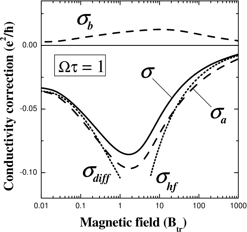
Figure 1: Conductivity correction (solid curve) at $\Omega\tau=1$, $\tau/\tau_{\phi}=0.01$. Dashed curves represent the backscattering ($\sigma_{a}$) and nonbackscattering ($\sigma_{b}$) contributions, dotted curves show the results of diffusion and high-field approximations.

In Fig. 1 weak-antilocalization correction to the conductivity for $\Omega\tau=1$ is shown by a solid line. In low fields the conductivity decreases and reaches a minimum at some $B=B_{min}$. Then the field dependence asymptotically tends to zero. Dashed curves in Fig. 1 represent the backscattering ($\sigma_{a}$) and nonbackscattering ($\sigma_{b}$) contributions. One can see that $\sigma_{b}$ can reach almost 25% of $|\sigma_{a}|$, therefore the nonbackscattering correction should be taken into account when fitting experimental data. The dotted curves in Fig. 1 show results of the diffusion and high-field approximations.sigma_diff One can see that the former is valid in a narrow region $B<0.5~{}B_{tr}$. The high-field asymptotic holds true only for $B>100~{}B_{tr}$. This proves importance of non-diffusion theory for high-mobility structures.

In Fig. 2 the conductivity correction is plotted for different strengths of spin-orbit interaction. One can see that for $\Omega\tau\lesssim 1$, in accordance with results of the previous Section, $\sigma(B)$ coincides with the zero-$\Omega$ dependence for $B>B_{min}$. The asymptotic $\sigma_{hf}(B)$ is reached at $B\approx 100~{}B_{tr}$ for all finite values of $\Omega\tau$. The positions of minima in the curves are shown in the inset. One can see that $B_{min}$ almost linearly depends on the spin splitting at $\Omega\tau>0.8$. Fitting yields the following approximate law

$$B_{min}\approx(3.9\>\Omega\tau-2)B_{tr}.$$

In the limit $\Omega\tau\rightarrow\infty$, the triplet state with $m_{s}=0$ does not contribute to the conductivity. The corresponding dependence is presented in Fig. 2. One can see a decrease of conductivity in the whole range of magnetic fields. At $B\gg B_{tr}$, the correction tends to zero as $0.035\>{e^{2}/\hbar}\>\sqrt{B_{tr}/B}$.

Figure 2: Conductivity correction for different strengths of spin-orbit interaction at $\tau/\tau_{\phi}=0.01$. The inset represents the positions of minima in the magnetoconductivity.

In experiments, the difference $\Delta\sigma(B)=\sigma(B)-\sigma(0)$ is measured. Since $\sigma(B)$ tends to zero at $B\to\infty$ for any $\Omega\tau$, one can extract $\sigma(0)$ from the saturation value of $\Delta\sigma$ at $B\to\infty$. In Fig. 3 the zero-field value of the conductivity correction $\sigma(0)$ is plotted as a function of $\Omega\tau$.

Figure 3: Zero-field correction to the conductivity for $\tau/\tau_{\phi}=0.01$ (solid curve). Dashed curves represent the backscattering ($\sigma_{a}$) and nonbackscattering ($\sigma_{b}$) contributions.

Fig. 3 shows how spin-orbit interaction changes the sign of weak-localization correction to conductivity. At $\Omega\tau=0$, all three triplet states and a singlet one yield contributions of the same absolute value. As a result, the zero-field correction is given by

$$\sigma_{a}^{0}(0)=-{e^{2}\over 2\pi^{2}\hbar}\ln{\tau_{\phi}\over\tau},\>\>\>\>\sigma_{b}^{0}(0)={e^{2}\over 2\pi^{2}\hbar}\ln{2}.$$

In the opposite limit $\Omega\tau\to\infty$, the triplet contribution is partially suppressed by the spin-orbit interaction. Calculation shows that the corrections reach the following values

$$\sigma_{a}^{\infty}(0)={e^{2}\over 4\pi^{2}\hbar}\left(0.57+\ln{\tau_{\phi}\over\tau}\right),\>\>\>\sigma_{b}^{\infty}(0)=-0.43{e^{2}\over 4\pi^{2}\hbar}.$$ (25)

One can see that $\sigma(0)$ changes its sign and reduces its absolute value when $\Omega\tau$ increases from zero to infinity.

It follows from Fig. 3 that the magnetoconductivity $\Delta\sigma(B)$ is an alternating function at small $\Omega\tau$, while at large values of the spin splitting $\Delta\sigma(B)$ is negative in the whole range of classically weak magnetic fields.

V Conclusion

In the present paper the anomalous magnetoresistance is calculated for 2D systems with only Rashba or only Dresselhaus spin-orbit interaction. In both cases the spin splitting is isotropic in $\bm{k}$-space and characterized by one constant $\Omega$. In the presence of both types of spin-orbit interaction, Eqs.(3), (5), and (7)-(11) hold true with ${\bm{\omega}}={\bm{\omega}}_{R}+{\bm{\omega}}_{D}$. However $P_{T}(N,N^{\prime})$ is not divided into finite blocks as Eq.(II), and one should use an infinite matrix for calculation of the triplet contribution to the conductivity in this case.

The problem has an analytic solution if the Rashba and Dresselhaus spin splittings are equal to each other. In this case the magnetoconductivity is positive in the whole range of magnetic fields like in systems without spin-orbit interaction. This result has been previously obtained in the diffusion approximation for $B\ll B_{tr}$.PikusPikus For magnetic field of arbitrary strength, the dependence $\sigma(B)$ is given by Eqs.(18), (19). This can be proved by noting that at $\Omega_{R}=\Omega_{D}$ the vector ${\bm{\Omega}}({\bm{k}})$ is directed along the same axis for all $\bm{k}$. As a result, the energy spectrum consists of two identical paraboloids shifted relative to each other in the direction of $\bm{\Omega}$.STNS Both these spin subbands independently yield equal conductivity corrections coinciding with those for spinless case. The same result takes place for symmetrical [110]- and [113]-grown quantum wells.

Application of an in-plane magnetic field ${\bm{B}}_{\parallel}$ destroys weak antilocalization. It has been demonstrated experimentally that the magnetoconductivity minimum disappears in the presence of ${\bm{B}}_{\parallel}$.tilted ; Nitta_B_par Weak antilocalization in a tilted magnetic field can be also described by the present theory. Parallel field influences the anomalous magnetoresistance due to two microscopic reasons. First, an in-plane field results in additional dephasing due to orbital effects.Malsh1 ; Meyer They can be taken into account as $B_{\parallel}$-dependent corrections to $\tau_{\phi}$. Second, an in-plane field induces finite Zeeman splitting. This results in a mixing of the singlet and triplet states,Malsh1 which makes the matrix $P(N,N^{\prime})$ in Eq.(10) infinite. However if the Zeeman splitting is much smaller than $\hbar\Omega$, then $B_{\parallel}$ affects only the singlet state. It leads to another correction to $\tau_{\phi}$ which should be taken into account only in ${\cal C}_{S}$, Eq.(11). Both the Zeeman and the orbital corrections to the dephasing rate can be extracted from the fit of experimental data by Eqs.(16), (17). Inclusion of the dephasing corrections into Eqs.(III), (24) allows one to describe anomalous magnetoresistance in pure in-plane field as well.

In conclusion, the theory of weak antilocalization is developed for high-mobility 2D systems. Anomalous magnetoconductivity is calculated in the whole range of classically weak fields and for arbitrary values of spin-orbit splitting.

References

• (1) B. L. Altshuler and A. G. Aronov, in Electron-electron interactions in disordered systems, edited by A.L. Efros and M. Pollak, (Elsevier, Amsterdam, 1985).
• (2) V. M. Gasparyan and A. Yu. Zyuzin, Fiz. Tverd. Tela 27, 1662 (1985) [Sov. Phys. Solid State 27, 999 (1985)].
• (3) S. V. Iordanskii, Yu. B. Lyanda-Geller and G. E. Pikus, Pis’ma Zh. Eksp. Teor. Fiz. 60, 199 (1994) [JETP Lett. 60, 206 (1994)].
• (4) M. A. Brand, A. Malinowski, O. Z. Karimov, P. A. Marsden, R. T. Harley, A. J. Shields, D. Sanvitto, D. A. Ritchie, and M. Y. Simmons Phys. Rev. Lett. 89, 236601 (2002).
• (5) T. Koga, J. Nitta, T. Akazaki, and H. Takayanagi, Phys. Rev. Lett. 89, 46801 (2002).
• (6) J. B. Miller, D. M. Zumbühl, C. M. Marcus, Y. B. Lyanda-Geller, D. Goldhaber-Gordon, K. Campman, and A. C. Gossard, Phys. Rev. Lett. 90, 076807 (2003).
• (7) C. Schierholz, T. Matsuyama, U. Merkt, and G. Meier, Phys. Rev. B70, 233311 (2004).
• (8) S. A. Studenikin, P. T. Coleridge, N. Ahmed, P. J. Poole, and A. Sachrajda, Phys. Rev. B 68, 035317 (2003).
• (9) S. A. Tarasenko and N. S. Averkiev, Pis’ma Zh. Eksp. Teor. Fiz. 75, 669 (2002) [JETP Lett. 75, 552 (2002)].
• (10) É. I. Rashba, Fiz. Tverd. Tela 2, 1224 (1960) [Sov. Phys. Solid State 2, 1109 (1960)].
• (11) I. S. Lyubinskiy and V. Yu. Kachorovskii, Phys. Rev. B 70, 205335 (2004).
• (12) A. P. Dmitriev, V. Yu. Kachorovskii, and I. V. Gornyi, Phys. Rev. B 56, 9910 (1997).
• (13) The zero-field value $F_{T}(0)$ is a small constant which should be extracted from $\Delta\sigma_{diff}$ as it has been done in Ref. tilted, .
• (14) G. M. Minkov, A. V. Germanenko, O. E. Rut, A. A. Sherstobitov, L. E. Golub, B. N. Zvonkov, and M. Willander, Phys. Rev. B70, 155323 (2004).
• (15) M. A. Skvortsov, JETP Lett. 67, 133 (1998); I. V. Gornyi, A. P. Dmitriev, and V. Yu. Kachorovskii, JETP Lett. 68, 338 (1998).
• (16) $\sigma_{diff}(B)$ is calculated as $\Delta\sigma_{diff}(B)+\sigma(0)$, with use of Eqs. (20) and (III), (24).
• (17) F.G. Pikus and G.E. Pikus, Phys. Rev. B 51, 16928 (1995).
• (18) F. E. Meijer, A. F. Morpurgo, T. M. Klapwijk, T. Koga, and J. Nitta Phys. Rev. B 70, 201307 (2004).
• (19) A. G. Mal’shukov, K. A. Chao, and M. Willander, Phys. Rev. B 56, 6436 (1997).
• (20) J.S. Meyer, A. Altland, and B.L. Altshuler, Phys. Rev. Lett. 89, 206601 (2002).