Bose-Einstein Condensation
as a Quantum Phase Transition
in an Optical Lattice^∗

Abstract

One of the most remarkable recent developments in the study of ultracold Bose gases is the observation of a reversible transition from a Bose Einstein condensate to a state composed of localized atoms as the strength of a periodic, optical trapping potential is varied. In [1] a model of this phenomenon has been analyzed rigorously. The gas is a hard core lattice gas and the optical lattice is modeled by a periodic potential of strength $\lambda$. For small $\lambda$ and temperature Bose-Einstein condensation (BEC) is proved to occur, while at large $\lambda$ BEC disappears, even in the ground state, which is a Mott-insulator state with a characteristic gap. The inter-particle interaction is essential for this effect. This contribution gives a pedagogical survey of these results.

1 Introduction

One of the most remarkable recent developments in the study of ultracold Bose gases is the observation of a reversible transition from a Bose-Einstein condensate to a state composed of localized atoms as the strength of a periodic, optical trapping potential is varied [2, 3]. This is an example of a quantum phase transition [4] where quantum fluctuations and correlations rather than energy-entropy competition is the driving force and its theoretical understanding is quite challenging. The model usually considered for describing this phenomenon is the Bose-Hubbard model and the transition is interpreted as a transition between a superfluid and a Mott insulator that was studied in [5] with an application to ${\rm He}^{4}$ in porous media in mind. The possibility of applying this scheme to gases of alkali atoms in optical traps was first realized in [6]. The article [7] reviews these developments and many recent papers, e.g., [8, 9, 10, 11, 12, 13, 14, 15, 16] are devoted to this topic. These papers contain also further references to earlier work along these lines.

The investigations of the phase transition in the Bose-Hubbard model are mostly based on variational or numerical methods and the signal of the phase transition is usually taken to be that an ansatz with a sharp particle number at each lattice site leads to a lower energy than a delocalized Bogoliubov state. On the other hand, there exists no rigorous proof, so far, that the true ground state of the model has off-diagonal long range order at one end of the parameter regime that disappears at the other end. In this contribution, which is based on the paper [1], we study a slightly different model where just this phenomenon can be rigorously proved and which, at the same time, captures the salient features of the experimental situation.

Physically, we are dealing with a trapped Bose gas with short range interaction. The model we discuss, however, is not a continuum model but rather a lattice gas, i.e., the particles are confined to move on a $d$-dimensional, hypercubic lattice and the kinetic energy is given by the discrete Laplacian. Moreover, when discusssing BEC, it is convenient not to fix the particle number but to work in a grand-canonical ensemble. The chemical potential is fixed in such a way that the average particle number equals half the number of lattice sites, i.e., we consider half filling. (This restriction is dictated by our method of proof.) The optical lattice is modeled by a periodic, one-body potential. In experiments the gas is enclosed in an additional trap potential that is slowly varying on the scale of the optical lattice but we neglect here the inhomogeneity due to such a potential and consider instead the thermodynamic limit.

In terms of bosonic creation and annihilation operators, $a^{\dagger}_{\bf x}$ and $a^{\phantom{\dagger}}_{\bf x}$, our Hamiltonian is expressed as

$$H=-\mbox{$\frac{1}{2}$}\sum_{\langle{{\bf x}}{{\bf y}}\rangle}(a^{\dagger}_{{\bf x}}a^{\phantom{\dagger}}_{{\bf y}}+a^{\phantom{\dagger}}_{{\bf x}}a^{\dagger}_{{\bf y}})+\lambda\sum_{{\bf x}}(-1)^{{\bf x}}a^{\dagger}_{{\bf x}}a^{\phantom{\dagger}}_{{\bf x}}+U\sum_{{\bf x}}a^{\dagger}_{{\bf x}}a^{\phantom{\dagger}}_{{\bf x}}(a^{\dagger}_{{\bf x}}a^{\phantom{\dagger}}_{{\bf x}}-1).$$ (1)

The sites ${{\bf x}}$ are in a cube $\Lambda\subset\mathbb{Z}^{d}$ with opposite sides identified (i.e., a $d$-dimensional torus) and $\langle{{\bf x}}{{\bf y}}\rangle$ stands for pairs of nearest neighbors. Units are chosen such that $\hbar^{2}/m=1$.

The first term in (1) is the discrete Laplacian $\sum_{\langle{{\bf x}}{{\bf y}}\rangle}(a^{\dagger}_{\bf x}-a^{\dagger}_{\bf y})(a^{\phantom{\dagger}}_{\bf x}-a^{\phantom{\dagger}}_{\bf y})$ minus $2d\sum_{{\bf x}}a^{\dagger}_{{\bf x}}a^{\phantom{\dagger}}_{\bf x}$, i.e., we have subtracted a chemical potential that equals $d$.

The optical lattice gives rise to a potential $\lambda(-1)^{{\bf x}}$ which alternates in sign between the $A$ and $B$ sublattices of even and odd sites. The inter-atomic on-site repulsion is $U$, but we consider here only the case of a hard-core interaction, i.e., $U=\infty$. If $\lambda=0$ but $U<\infty$ we have the Bose-Hubbard model. Then all sites are equivalent and the lattice represents the attractive sites of the optical lattice. In our case the adjustable parameter is $\lambda$ instead of $U$ and for large $\lambda$ the atoms will try to localize on the $B$ sublattice. The Hamiltonian (1) conserves the particle number $N$ and it can be shown that, for $U=\infty$, the lowest energy is obtained uniquely for $N=\mbox{$\frac{1}{2}$}|\Lambda|$, i.e., half the number of lattice sites. Because of the periodic potential the unit cell in this model consists of two lattice sites, so that we have on average one particle per unit cell. This corresponds, physically, to filling factor 1 in the Bose-Hubbard model.

For given temperature $T$, we consider grand-canonical thermal equilibrium states, described by the Gibbs density matrices $Z^{-1}\exp(-\beta H)$ with $Z$ the normalization factor (partition function) and $\beta=1/T$ the inverse temperature. Units are chosen so that Boltzmann’s constant equals 1. The thermal expectation value of some observable $\mathcal{O}$ will be denoted by $\langle{\mathcal{O}}\rangle=Z^{-1}{\rm Tr}\,{\mathcal{O}}\exp(-\beta H)$.

Our main results about this model can be summarized as follows:

• If $T$ and $\lambda$ are both small, there is Bose-Einstein condensation. In this parameter regime the one-body density matrix $\gamma({\bf x},{\bf y})=\langle a^{\dagger}_{\bf x}a^{\phantom{\dagger}}_{\bf y}\rangle$ has exactly one large eigenvalue (in the thermodynamic limit), and the corresponding condensate wave function is $\phi({\bf x})=$constant.

• If either $T$ or $\lambda$ is big enough, then the one-body density matrix decays exponentially with the distance $|{\bf x}-{\bf y}|$, and hence there is no BEC. In particular, this applies to the ground state $T=0$ for $\lambda$ big enough, where the system is in a Mott insulator phase.

• The Mott insulator phase is characterized by a gap, i.e., a jump in the chemical potential. We are able to prove this, at half-filling, in the region described in item 2 above. More precisely, there is a cusp in the dependence of the ground state energy on the number of particles; adding or removing one particle costs a non-zero amount of energy. We also show that there is no such gap whenever there is BEC.

• The interparticle interaction is essential for items 2 and 3. Non-interacting bosons always display BEC for low, but positive $T$ (depending on $\lambda$, of course).

• For all $T\geq 0$ and all $\lambda>0$ the diagonal part of the one-body density matrix $\langle a^{\dagger}_{\bf x}a^{\phantom{\dagger}}_{\bf x}\rangle$ (the one-particle density) is not constant. Its value on the A sublattice is constant, but strictly less than its constant value on the B sublattice and this discrepancy survives in the thermodynamic limit. In contrast, in the regime mentioned in item 1, the off-diagonal long-range order is constant, i.e., $\langle a^{\dagger}_{\bf x}a^{\phantom{\dagger}}_{\bf y}\rangle\approx\phi({\bf x})\phi({\bf y})^{*}$ for large $|{\bf x}-{\bf y}|$ with $\phi({\bf x})=$constant.

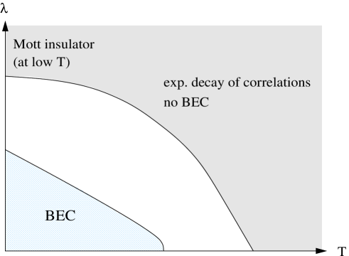
Figure 1: Schematic phase diagram at half-filling

Because of the hard-core interaction between the particles, there is at most one particle at each site and our Hamiltonian (with $U=\infty$) thus acts on the Hilbert space ${\mathcal{H}}=\bigotimes_{{\bf x}\in\Lambda}{\mathbb{C}}^{2}$. The creation and annihilation operators can be represented as $2\times 2$ matrices with

$$a^{\dagger}_{{{\bf x}}}\leftrightarrow\left(\begin{array}[]{cc}0&1\\ 0&0\end{array}\right),\quad a^{\phantom{\dagger}}_{{{\bf x}}}\leftrightarrow\left(\begin{array}[]{cc}0&0\\ 1&0\end{array}\right),\quad a^{\dagger}_{{{\bf x}}}a^{\phantom{\dagger}}_{{\bf x}}\leftrightarrow\left(\begin{array}[]{cc}1&0\\ 0&0\end{array}\right),$$

for each ${{\bf x}}\in\Lambda$. More precisely, these matrices act on the tensor factor associated with the site ${\bf x}$ while $a^{\dagger}_{{{\bf x}}}$ and $a^{\phantom{\dagger}}_{{{\bf x}}}$ act as the identity on the other factors in the Hilbert space ${\mathcal{H}}=\bigotimes_{{\bf x}\in\Lambda}{\mathbb{C}}^{2}$.

The Hamiltonian can alternatively be written in terms of the spin 1/2 operators

$$S^{1}=\frac{1}{2}\left(\begin{array}[]{cc}0&1\\ 1&0\end{array}\right),\quad S^{2}=\frac{1}{2}\left(\begin{array}[]{cc}0&-{\rm i}\\ {\rm i}&0\end{array}\right),\quad S^{3}=\frac{1}{2}\left(\begin{array}[]{cc}1&0\\ 0&-1\end{array}\right).$$

The correspondence with the creation and annihilation operators is

$$a^{\dagger}_{{{\bf x}}}=S^{1}_{{{\bf x}}}+{\rm i}S^{2}_{{{\bf x}}}\equiv S_{{\bf x}}^{+},\quad a^{\phantom{\dagger}}_{{{\bf x}}}=S^{1}_{{{\bf x}}}-{\rm i}S^{2}_{{{\bf x}}}\equiv S_{{\bf x}}^{-},$$

and hence $a^{\dagger}_{{{\bf x}}}a^{\phantom{\dagger}}_{{{\bf x}}}=S_{{\bf x}}^{3}+\mbox{$\frac{1}{2}$}$. (This is known as the Matsubara-Matsuda correspondence [17].) Adding a convenient constant to make the periodic potential positive, the Hamiltonian (1) for $U=\infty$ is thus equivalent to

$$H = -\mbox{$\frac{1}{2}$}\sum_{\langle{{\bf x}}{{\bf y}}\rangle}(S^{+}_{{\bf x}}S^{-}_{{\bf y}}+S^{-}_{{\bf x}}S^{+}_{{\bf y}})+\lambda\sum_{{\bf x}}\left[\mbox{$\frac{1}{2}$}+(-1)^{{\bf x}}S^{3}_{{\bf x}}\right]$$ (2)

$$= -\sum_{\langle{{\bf x}}{{\bf y}}\rangle}(S^{1}_{{\bf x}}S^{1}_{{\bf y}}+S^{2}_{{\bf x}}S^{2}_{{\bf y}})+\lambda\sum_{{\bf x}}\left[\mbox{$\frac{1}{2}$}+(-1)^{{\bf x}}S^{3}_{{\bf x}}\right].$$

Without loss of generality we may assume $\lambda\geq 0$. This Hamiltonian is well known as a model for interacting spins, referred to as the XY model [18]. The last term has the interpretation of a staggered magnetic field. We note that BEC for the lattice gas is equivalent to off-diagonal long range order for the 1- and 2-components of the spins.

The Hamiltonian (2) is clearly invariant under simultaneous rotations of all the spins around the 3-axis. In particle language this is the $U(1)$ gauge symmetry associated with particle number conservation of the Hamiltonian (1). Off-diagonal long range order (or, equivalently, BEC) implies that this symmetry is spontaneously broken in the state under consideration. It is notoriously difficult to prove such symmetry breaking for systems with a continuous symmetry. One of the few available techniques is that of reflection positivity (and the closely related property of Gaussian domination) and fortunately it can be applied to our system. For this, however, the hard core and half-filling conditions are essential because they imply a particle-hole symmetry that is crucial for the proofs to work. Naturally, BEC is expected to occur at other fillings, but no one has so far found a way to prove condensation (or, equivalently, long-range order in an antiferromganet with continuous symmetry) without using reflection positivity and infrared bounds, and these require the addtional symmetry.

Reflection positivity was first formulated by K. Osterwalder and R. Schrader [19] in the context of relativistic quantum field theory. Later, J. Fröhlich, B. Simon and T. Spencer used the concept to prove the existence of a phase transition for a classical spin model with a continuous symmetry [20], and E. Lieb and J. Fröhlich [21] as well as F. Dyson, E. Lieb and B. Simon [18] applied it for the analysis of quantum spin systems. The proof of off-diagonal long range order for the Hamiltonian (2) (for small $\lambda$) given here is based on appropriate modifications of the arguments in [18].

2 Reflection Positivity

In the present context reflection positivity means the following. We divide the torus $\Lambda$ into two congruent parts, $\Lambda_{\rm L}$ and $\Lambda_{\rm R}$, by cutting it with a hyperplane orthogonal to one of the $d$ directions. (For this we assume that the side length of $\Lambda$ is even.) This induces a factorization of the Hilbert space, ${\mathcal{H}}={\mathcal{H}}_{\rm L}\otimes{\mathcal{H}}_{\rm R}$, with

$${\mathcal{H}}_{\rm L,R}=\bigotimes_{{\bf x}\in\Lambda_{\rm L,R}}{\mathbb{C}}^{2}.$$

There is a natural identification between a site ${\bf x}\in\Lambda_{\rm L}$ and its mirror image $\vartheta{\bf x}\in\Lambda_{\rm R}$. If $F$ is an operator on ${\mathcal{H}}={\mathcal{H}}_{\rm L}$ we define its reflection $\theta F$ as an operator on ${\mathcal{H}}_{\rm R}$ in the following way. If $F=F_{\bf x}$ operates non-trivially only on one site, ${\bf x}\in\Lambda_{\rm L}$, we define $\theta F=VF_{\vartheta{\bf x}}V^{\dagger}$ where $V$ denotes the unitary particle-hole transformation or, in the spin language, rotation by $\pi$ around the 1-axis. This definition extends in an obvious way to products of operators on single sites and then, by linearity, to arbitrary operators on ${\mathcal{H}}_{\rm L}$. Reflection positivity of a state $\langle\,\cdot\,\rangle$ means that

$$\langle F\theta\overline{F}\rangle\geq 0$$ (3)

for any $F$ operating on ${\mathcal{H}}_{\rm L}$. Here $\overline{F}$ is the complex conjugate of the operator $F$ in the matrix representation defined above, i.e., defined by the basis where the operators $S^{3}_{{\bf x}}$ are diagonal.

We now show that reflection positivity holds for any thermal equilibrium state of our Hamiltonian. We can write the Hamiltonian (2) as

$$H=H_{\rm L}+H_{\rm R}-\mbox{$\frac{1}{2}$}\sum_{\langle{{\bf x}}{{\bf y}}\rangle\in M}(S^{+}_{{\bf x}}S^{-}_{{\bf y}}+S^{-}_{{\bf x}}S^{+}_{{\bf y}}),$$ (4)

where $H_{\rm L}$ and $H_{\rm R}$ act non-trivially only on ${\mathcal{H}}_{\rm L}$ and ${\mathcal{H}}_{\rm R}$, respectively. Here, $M$ denotes the set of bonds going from the left sublattice to the right sublattice. (Because of the periodic boundary condition these include the bonds that connect the right boundary with the left boundary.) Note that $H_{\rm R}=\theta H_{\rm L}$, and

$$\sum_{\langle{{\bf x}}{{\bf y}}\rangle\in M}(S^{+}_{{\bf x}}S^{-}_{{\bf y}}+S^{-}_{{\bf x}}S^{+}_{{\bf y}})=\sum_{\langle{{\bf x}}{{\bf y}}\rangle\in M}(S^{+}_{{\bf x}}\theta S^{+}_{{\bf x}}+S^{-}_{{\bf x}}\theta S^{-}_{{\bf x}}).$$

For these properties it is essential that we included the unitary particle-hole transformation $V$ in the definition of the reflection $\theta$. For reflection positivity it is also important that all operators appearing in $H$ (4) have a real matrix representation. Moreover, the minus sign in (4) is essential.

Using the Trotter product formula, we have

$${\rm Tr}\,F\theta\overline{F}e^{-\beta H}=\\ \lim_{n\to\infty}{\rm Tr}\,F\theta\overline{F}\,{\mathcal{Z}}_{n}$$

with

$${\mathcal{Z}}_{n}=\left[e^{-\frac{1}{n}\beta H_{L}}\theta e^{-\frac{1}{n}\beta H_{L}}\prod_{\langle{{\bf x}}{{\bf y}}\rangle\in M}\left(1+\frac{\beta}{2n}\left[S^{+}_{{\bf x}}\theta S^{+}_{{\bf x}}+S^{-}_{{\bf x}}\theta S^{-}_{{\bf x}})\right]\right)\right]^{n}.$$ (5)

Observe that ${\mathcal{Z}}_{n}$ is a sum of terms of the form

$$\mbox{$\prod_{i}$}A_{i}\theta A_{i},$$ (6)

with $A_{i}$ given by either $e^{-\frac{1}{n}\beta H_{L}}$ or $\sqrt{\frac{\beta}{2n}}S^{+}_{{\bf x}}$ or $\sqrt{\frac{\beta}{2n}}S^{-}_{{\bf x}}$. All the $A_{i}$ are real matrices, and therefore

$${\rm Tr}_{\mathcal{H}}\,F\theta\overline{F}\,\mbox{$\prod_{i}$}A_{i}\theta A_{i}={\rm Tr}_{\mathcal{H}}\,F\mbox{$\prod_{i}$}A_{i}\,\theta\left[\overline{F}\mbox{$\prod_{j}$}A_{j}\right]=\big{|}{\rm Tr}_{{\mathcal{H}}_{\rm L}}\,F\mbox{$\prod_{i}$}A_{i}\big{|}^{2}\geq 0.$$ (7)

Hence ${\rm Tr}\,F\theta\overline{F}\,{\mathcal{Z}}_{n}$ is a sum of non-negative terms and therefore non-negative. This proves our assertion.

3 Proof of BEC for Small $\lambda$ and $T$

The main tool in our proof of BEC are infrared bounds. More precisely, for ${\bf p}\in\Lambda^{*}$ (the dual lattice of $\Lambda$), let $\widetilde{S}^{\#}_{\bf p}=|\Lambda|^{-1/2}\sum_{\bf x}S_{\bf x}^{\#}\exp({\rm i}{\bf p}\cdot{\bf x})$ denote the Fourier transform of the spin operators. We claim that

$$(\widetilde{S}_{\bf p}^{1},\widetilde{S}^{1}_{-{\bf p}})\leq\frac{T}{2E_{{\bf p}}},$$ (8)

with $E_{{\bf p}}=\sum_{i=1}^{d}(1-\cos(p_{i}))$. Here, $p_{i}$ denotes the components of ${{\bf p}}$, and $(\,,\,)$ denotes the Duhamel two point function at temperature $T$, defined by

$$(A,B)=\int_{0}^{1}{\rm Tr}\,\left(Ae^{-s\beta H}Be^{-(1-s)\beta H}\right)ds/{\rm Tr}\,e^{-\beta H}$$ (9)

for any pair of operators $A$ and $B$. Because of invariance under rotations around the $S^{3}$ axis, (8) is equally true with $S^{1}$ replaced by $S^{2}$, of course.

The crucial lemma (Gaussian domination) is the following. Define, for a complex valued function $h$ on the bonds $\langle{{\bf x}}{{\bf y}}\rangle$ in $\Lambda$,

$$Z(h)={\rm Tr}\,\exp\left[-\beta K(h)\right],$$ (10)

with $K(h)$ the modified Hamiltonian

$$K(h)=\frac{1}{4}\sum_{\langle{{\bf x}}{{\bf y}}\rangle}\left(\big{(}S^{+}_{{\bf x}}-S^{-}_{{\bf y}}-h_{{{\bf x}}{{\bf y}}}\big{)}^{2}+\big{(}S^{-}_{{\bf x}}-S^{+}_{{\bf y}}-\overline{h_{{{\bf x}}{{\bf y}}}}\big{)}^{2}\right)+\lambda\sum_{{\bf x}}\big{[}\mbox{$\frac{1}{2}$}+(-1)^{{\bf x}}S^{3}_{{\bf x}}\big{]}.$$ (11)

Note that for $h\equiv 0$, $K(h)$ agrees with the Hamiltonian $H$, because $(S^{\pm})^{2}=0$. We claim that, for any real valued $h$,

$$Z(h)\leq Z(0).$$ (12)

The infrared bound then follows from $d^{2}Z(\varepsilon h)/d\varepsilon^{2}|_{\varepsilon=0}\leq 0$, taking $h_{{\bf x}{\bf y}}=\exp({\rm i}{\bf p}\cdot{\bf x})-\exp({\rm i}{\bf p}\cdot{\bf y})$. This is not a real function, though, but the negativity of the (real!) quadratic form $d^{2}Z(\varepsilon h)/d\varepsilon^{2}|_{\varepsilon=0}$ for real $h$ implies negativity also for complex-valued $h$.

The proof of (12) is very similar to the proof of the reflection positivity property (3) given above. It follows along the same lines as in [18], but we repeat it here for convenience of the reader.

The intuition behind (12) is the following. First, in maximizing $Z(h)$ one can restrict to gradients, i.e., $h_{{\bf x}{\bf y}}=\hat{h}_{\bf x}-\hat{h}_{\bf y}$ for some function $\hat{h}_{\bf x}$ on $\Lambda$. (This follows from stationarity of $Z(h)$ at a maximizer $h_{\rm max})$.) Reflection positivity implies that $\langle A\theta\overline{B}\rangle$ defines a scalar product on operators on $\mathcal{H}_{\rm L}$, and hence there is a corresponding Schwarz inequality. Moreover, since reflection positivity holds for reflections across any hyperplane, one arrives at the so-called chessboard inequality, which is simply a version of Schwarz’s inequality for multiple reflections across different hyperplanes. Such a chessboard estimate implies that in order to maximize $Z(h)$ it is best to choose the function $\hat{h}_{{\bf x}}$ to be constant. In the case of classical spin systems [20], this intuition can be turned into a complete proof of (12). Because of non-commutativity of $K(h)$ with $K(0)=H$, this is not possible in the quantum case. However, one can proceed by using the Trotter formula as follows.

Let $h_{\rm max}$ be a function that maximizes $Z(h)$ for real valued $h$. If there is more than one maximizer, we choose $h_{\rm max}$ to be one that vanishes on the largest number of bonds. We then have to show that actually $h_{\rm max}\equiv 0$. If $h_{\rm max}\not\equiv 0$, we draw a hyperplane such that $h_{{{\bf x}}{{\bf y}}}\neq 0$ for at least one pair $\langle{{\bf x}}{{\bf y}}\rangle$ crossing the plane. We can again write

$$K(h)=K_{L}(h)+K_{R}(h)+\frac{1}{4}\sum_{\langle{{\bf x}}{{\bf y}}\rangle\in M}\left((S^{+}_{{\bf x}}-S^{-}_{{\bf y}}-h_{{{\bf x}}{{\bf y}}})^{2}+(S^{-}_{{\bf x}}-S^{+}_{{\bf y}}-h_{{{\bf x}}{{\bf y}}})^{2}\right).$$ (13)

Using the Trotter formula, we have $Z(h)=\lim_{n\to\infty}\alpha_{n}$, with

$$\alpha_{n}={\rm Tr}\,\left[e^{-\beta K_{L}/n}e^{-\beta K_{R}/n}\prod_{\langle{\bf x}{\bf y}\rangle\in M}e^{-\beta(S^{+}_{{\bf x}}-S^{-}_{{\bf y}}-h_{{{\bf x}}{{\bf y}}})^{2}/4n}e^{-\beta(S^{-}_{{\bf x}}-S^{+}_{{\bf y}}-h_{{{\bf x}}{{\bf y}}})^{2}/4n}\right]^{n}.$$ (14)

For any matrix, we can write

$$e^{-D^{2}}=(4\pi)^{-1/2}\int_{\mathbb{R}}dk\,e^{{\rm i}kD}e^{-k^{2}/4}.$$ (15)

If we apply this to the last two factors in (14), and note that $S^{-}_{\bf y}=\theta S^{+}_{\bf x}$ if $\langle{\bf x}{\bf y}\rangle\in M$. Denoting by ${\bf x}_{1},\dots,{\bf x}_{l}$ the points on the left side of the bonds in $M$, we have that

$$\alpha_{n} = (4\pi)^{-nl}\int_{R^{2nl}}d^{2nl}k\,{\rm Tr}\,\left[e^{-\beta K_{L}/n}e^{-\beta K_{R}/n}e^{{\rm i}k_{1}(S^{+}_{{\bf x}_{1}}-\theta S^{+}_{{\bf x}_{1}})\beta^{1/2}/2n^{1/2}}\dots\right]$$ (16)

$$\times e^{-k^{2}/4}e^{-{\rm i}k_{1}h_{{\bf x}_{1}\vartheta{\bf x}_{1}}\beta^{1/2}/2n^{1/2}\dots}.$$

Here we denotes $k^{2}=\sum k_{i}^{2}$ for short. Since matrices on the right of $M$ commute with matrices on the left, and since all matrices in question are real, we see that the trace in the integrand above can be written as

$${\rm Tr}\,\left[e^{-\beta K_{L}/n}e^{{\rm i}k_{1}S^{+}_{{\bf x}_{1}}\beta^{1/2}/2n^{1/2}}\dots\right]\overline{{\rm Tr}\,\left[e^{-\beta K_{R}/n}e^{{\rm i}k_{1}\theta S^{+}_{{\bf x}_{1}}\beta^{1/2}/2n^{1/2}}\dots\right]}.$$ (17)

Using the Schwarz inequality for the $k$ integration, and ‘undoing’ the above step, we see that

$$\!\!\!\!\!|\alpha_{n}|^{2}\!\!\! \leq \!\!\!\left((4\pi)^{-nl}\int_{R^{2nl}}d^{2nl}k\,e^{-k^{2}/4}\right.$$ (18)

$$\left.\quad\times{\rm Tr}\,\left[e^{-\beta K_{L}/n}e^{-\beta\theta K_{L}/n}e^{{\rm i}k_{1}(S^{+}_{{\bf x}_{1}}-\theta S^{+}_{{\bf x}_{1}})\beta^{1/2}/2n^{1/2}}\dots\right]\phantom{\int_{R^{2nl}}}\!\!\!\!\!\!\!\!\!\!\!\!\!\!\right)$$

$$\!\!\!\!\!\times\left((4\pi)^{-nl}\int_{R^{2nl}}d^{2nl}k\,e^{-k^{2}/4}\right.$$

$$\left.\quad\times{\rm Tr}\,\left[e^{-\beta\theta K_{R}/n}e^{-\beta K_{R}/n}e^{{\rm i}k_{1}(S^{+}_{{\bf x}_{1}}-\theta S^{+}_{{\bf x}_{1}})\beta^{1/2}/2n^{1/2}}\dots\right]\phantom{\int_{R^{2nl}}}\!\!\!\!\!\!\!\!\!\!\!\!\!\!\right).$$

In terms of the partition function $Z(h)$, this means that

$$|Z(h_{\rm max})|^{2}\leq Z(h^{(1)})Z(h^{(2)}),$$ (19)

where $h^{(1)}$ and $h^{(2)})$ are obtained from $h_{\rm max}$ by reflection across $M$, in the following way:

$$h^{(1)}_{{\bf x}{\bf y}}=\left\{\begin{array}[]{ll}h_{{\bf x}{\bf y}}&{\rm if\ }{\bf x},{\bf y}\in\Lambda_{L}\\ h_{\vartheta{\bf x}\vartheta{\bf y}}&{\rm if\ }{\bf x},{\bf y}\in\Lambda_{R}\\ 0&{\rm if\ }\langle{\bf x}{\bf y}\rangle\in M\end{array}\right.$$ (20)

and $h^{(2)}$ is given by the same expression, interchanging $L$ and $R$. Therefore also $h^{(1)}$ and $h^{(2)}$ must be maximizers of $Z(h)$. However, one of them will contain strictly more zeros than $h_{\rm max}$, since $h_{\rm max}$ does not vanish identically for bonds crossing $M$. This contradicts our assumption that $h_{\rm max}$ contains the maximal number of zeros among all maximizers of $Z(h)$. Hence $h_{\rm max}\equiv 0$ identically. This completes the proof of (12).

The next step is to transfer the upper bound on the Duhamel two point function (8) into an upper bound on the thermal expectation value. This involves convexity arguments and estimations of double commutators like in Section 3 in [18]. For this purpose, we have to evaluate the double commutators

$$[\widetilde{S}^{1}_{{\bf p}},[H,\widetilde{S}^{1}_{-{{\bf p}}}]]+[\widetilde{S}^{2}_{{\bf p}},[H,\widetilde{S}^{2}_{-{{\bf p}}}]]=-\frac{2}{|\Lambda|}\Big{(}H-\mbox{$\frac{1}{2}$}\lambda|\Lambda|+2\sum_{\langle{{\bf x}}{{\bf y}}\rangle}S^{3}_{{\bf x}}S^{3}_{{\bf y}}\cos{{\bf p}}\cdot({{\bf x}}-{{\bf y}})\Big{)}.$$ (21)

Let $C_{{\bf p}}$ denote the expectation value of this last expression,

$$C_{{\bf p}}=\langle[\widetilde{S}^{1}_{{\bf p}},[H,\widetilde{S}^{1}_{-{{\bf p}}}]]+[\widetilde{S}^{2}_{{\bf p}},[H,\widetilde{S}^{2}_{-{{\bf p}}}]]\rangle\geq 0.$$

The positivity of $C_{{\bf p}}$ can be seen from an eigenfunction-expansion of the trace. From [18, Corollary 3.2 and Theorem 3.2] and (8) we infer that

$$\langle\widetilde{S}_{{\bf p}}^{1}\widetilde{S}_{-{{\bf p}}}^{1}+\widetilde{S}_{{\bf p}}^{2}\widetilde{S}_{-{{\bf p}}}^{2}\rangle\leq\frac{1}{2}\sqrt{\frac{C_{{\bf p}}}{E_{{\bf p}}}}\coth\sqrt{\beta^{2}C_{{\bf p}}E_{{\bf p}}/4}.$$ (22)

Using $\coth x\leq 1+1/x$ and Schwarz’s inequality, we obtain for the sum over all ${{\bf p}}\neq{\bf 0}$,

$$\sum_{{{\bf p}}\neq{\bf 0}}\langle\widetilde{S}_{{\bf p}}^{1}\widetilde{S}_{-{{\bf p}}}^{1}+\widetilde{S}_{{\bf p}}^{2}\widetilde{S}_{-{{\bf p}}}^{2}\rangle\leq\frac{1}{\beta}\sum_{{{\bf p}}\neq{\bf 0}}\frac{1}{E_{{\bf p}}}+\frac{1}{2}\Big{(}\sum_{{{\bf p}}\neq{\bf 0}}\frac{1}{E_{{\bf p}}}\Big{)}^{1/2}\Big{(}\sum_{{{\bf p}}\neq{\bf 0}}C_{{\bf p}}\Big{)}^{1/2}.$$ (23)

We have $\sum_{{{\bf p}}\in\Lambda^{*}}C_{{\bf p}}=-2\langle H\rangle+\lambda|\Lambda|$, which can be bounded from above using the following lower bound on the Hamiltonian:

$$H\geq-\frac{|\Lambda|}{4}\left[d(d+1)+4\lambda^{2}\right]^{1/2}+\mbox{$\frac{1}{2}$}\lambda|\Lambda|.$$ (24)

This inequality follows from the fact that the lowest eigenvalue of

$$-\frac{1}{2}S_{{\bf x}}^{1}\sum_{i=1}^{2d}S_{{{\bf y}}_{i}}^{1}-\frac{1}{2}S_{{\bf x}}^{2}\sum_{i=1}^{2d}S_{{{\bf y}}_{i}}^{2}+\lambda S_{{\bf x}}^{3}$$ (25)

is given by $-\mbox{$\frac{1}{4}$}[d(d+1)+4\lambda^{2}]^{1/2}$. This can be shown exactly in the same way as [18, Theorem C.1]. Since the Hamiltonian $H$ can be written as a sum of terms like (25), with ${{\bf y}}_{i}$ the nearest neighbors of ${{\bf x}}$, we get from this fact the lower bound (24).

With the aid of the sum rule

$$\sum_{{{\bf p}}\in\Lambda^{*}}\langle\widetilde{S}_{{\bf p}}^{1}\widetilde{S}_{-{{\bf p}}}^{1}+\widetilde{S}_{{\bf p}}^{2}\widetilde{S}_{-{{\bf p}}}^{2}\rangle=\frac{|\Lambda|}{2}$$

(which follows from $(S^{1})^{2}=(S^{2})^{2}=1/4$), we obtain from (23) and (24) the following lower bound in the thermodynamic limit:

$$\lim_{\Lambda\to\infty}\frac{1}{|\Lambda|}\langle\widetilde{S}_{\bf 0}^{1}\widetilde{S}_{{\bf 0}}^{1}+\widetilde{S}_{\bf 0}^{2}\widetilde{S}_{{\bf 0}}^{2}\rangle$$

$$\geq\frac{1}{2}-\frac{1}{2}\left(\mbox{$\frac{1}{2}$}\left[d(d+1)+4\lambda^{2}\right]^{1/2}c_{d}\right)^{1/2}-\frac{1}{\beta}c_{d},$$ (26)

with $c_{d}$ given by

$$c_{d}=\frac{1}{(2\pi)^{d}}\int_{[-\pi,\pi]^{d}}d{{\bf p}}\frac{1}{E_{{\bf p}}}.$$ (27)

This is our final result. Note that $c_{d}$ is finite for $d\geq 3$. Hence the right side of (26) is positive, for large enough $\beta$, as long as

$$\lambda^{2}<\frac{1}{c_{d}^{2}}-\frac{d(d+1)}{4}.$$

In $d=3$, $c_{3}\approx 0.505$ [18], and hence this condition is fulfilled for $\lambda\lesssim 0.960$. In [18] it was also shown that $dc_{d}$ is monotone decreasing in $d$, which implies a similar result for all $d>3$.

The connection with BEC is as follows. Since $H$ is real, also $\gamma({{\bf x}},{{\bf y}})$ is real and we have

$$\gamma({{\bf x}},{{\bf y}})=\langle S_{{\bf x}}^{+}S_{{\bf y}}^{-}\rangle=\langle S_{{\bf x}}^{1}S_{{\bf y}}^{1}+S_{{\bf x}}^{2}S_{{\bf y}}^{2}\rangle.$$

Hence, if $\varphi_{0}=|\Lambda|^{-1/2}$ denotes the constant function,

$$\langle\varphi_{0}|\gamma|\varphi_{0}\rangle=\langle\widetilde{S}_{\bf 0}^{1}\widetilde{S}_{{\bf 0}}^{1}+\widetilde{S}_{\bf 0}^{2}\widetilde{S}_{{\bf 0}}^{2}\rangle,$$

and thus the bound (26) implies that the largest eigenvalue of $\gamma({\bf x},{\bf y})$ is bounded from below by the right side of (26). In addition one can show that the infrared bounds imply that there is at most one large eigenvalue (of the order $|\Lambda|$), and that the corresponding eigenvector (the ‘condensate wave function’) is strictly constant in the thermodynamic limit [1]. The constancy of the condensate wave function is surprising and is not expected to hold for densities different from $\frac{1}{2}$, where particle-hole symmetry is absent. In contrast to the condensate wave function the particle density shows the staggering of the periodic potential [1, Thm. 3]. It also contrasts with the situation for zero interparticle interaction, as discussed at the end of this paper.

In the BEC phase there is no gap for adding particles beyond half filling (in the thermodynamic limit): The ground state energy, $E_{k}$, for $\mbox{$\frac{1}{2}$}|\Lambda|+k$ particles satisfies

$$0\leq E_{k}-E_{0}\leq\frac{(\rm const.)}{|\Lambda|}$$ (28)

(with a constant that depends on $k$ but not on $|\Lambda|$.) The proof of (28) is by a variational calculation, with a trial state of the form $(\widetilde{S}^{+}_{\bf 0})^{k}|0\rangle$, where $|0\rangle$ denotes the absolute ground state, i.e., the ground state for half filling. (This is the unique ground state of the Hamiltonian, as can be shown using reflection positivity. See Appendix A in [1].) Also, in the thermodynamic limit, the energy per site for a given density, $e(\varrho)$, satisfies

$$e(\varrho)-e(\mbox{$\frac{1}{2}$})\leq{\rm const.\,}(\varrho-\mbox{$\frac{1}{2}$})^{2}.$$ (29)

Thus there is no cusp at $\varrho=1/2$. To show this, one takes a trial state of the form

$$|\psi_{\bf y}\rangle=e^{{\rm i}\varepsilon\sum_{\bf x}S_{\bf x}^{2}}(S_{\bf y}^{1}+\mbox{$\frac{1}{2}$})|0\rangle.$$ (30)

The motivation is the following: we take the ground state and first project onto a given direction of $S^{1}$ on some site ${{\bf y}}$. If there is long-range order, this should imply that essentially all the spins point in this direction now. Then we rotate slightly around the $S^{2}$-axis. The particle number should then go up by $\varepsilon|\Lambda|$, but the energy only by $\varepsilon^{2}|\Lambda|$. We refer to [1, Sect. IV] for the details.

The absence of a gap in the case of BEC is not surprising, since a gap is characteristic for a Mott insulator state. We show the occurrence of a gap, for large enough $\lambda$, in the next section.

4 Absence of BEC and Mott Insulator Phase

The main results of this section are the following: If either

• $\lambda\geq 0$ and $T>d/(2\ln 2)$, or

• $T\geq 0$ and $\lambda\geq 0$ such that $\lambda+|e(\lambda)|>d$, with $e(\lambda)=$ ground state energy per site,

then there is exponential decay of correlations:

$$\gamma({\bf x},{\bf y})\leq{\rm(const.)}\exp(-\kappa|{\bf x}-{\bf y}|)$$ (31)

with $\kappa>0$. Moreover, for $T=0$, the ground state energy in a sector of fixed particle number $N=\mbox{$\frac{1}{2}$}|\Lambda|+k$, denoted by $E_{k}$, satisfies

$$E_{k}+E_{-k}-2E_{0}\geq(\lambda+|e(\lambda)|-d)|k|.$$ (32)

I.e, for large enough $\lambda$ the chemical potential has a jump at half filling.

The derivation of these two properties is based on a path integral representation of the equilibrium state at temperature $T$, and of the ground state which is obtained in the limit $T\to\infty$. density matrix. The analysis starts from the observation that the density operator $e^{-\beta H}$ has non-negative matrix elements in the basis in which $\{S_{{\bf x}}^{3}\}$ are diagonal, i.e. of states with specified particle occupation numbers. It is convenient to focus on the dynamics of the ‘quasi-particles’ which are defined so that the presence of one at a site ${\bf x}$ signifies a deviation there from the occupation state which minimizes the potential-energy. Since the Hamiltonian is $H=H_{0}+\lambda W$, with $H_{0}$ the hopping term in (2) and $W$ the staggered field, we define the quasi-particle number operators $n_{\bf x}$ as:

$$n_{\bf x}\ =\ \mbox{$\frac{1}{2}$}+(-1)^{\bf x}S_{{\bf x}}^{3}=\begin{cases}a^{\dagger}_{{\bf x}}a_{{\bf x}}&\hbox{for ${\bf x}$ even}\\ 1-a^{\dagger}_{{\bf x}}a_{{\bf x}}&\hbox{for ${\bf x}$ odd}\end{cases}\,.$$ (33)

Thus $n_{{\bf x}}=1$ means presence of a particle if ${\bf x}$ is on the A sublattice (potential maximum) and absence if ${\bf x}$ is on the B sublattice (potential minimum).

The collection of the joint eigenstates of the occupation numbers, $\{|\{n_{\bf x}\}\rangle\}$, provides a convenient basis for the Hilbert space. The functional integral representation of $\langle\{n_{\bf x}\}|\,e^{-\beta(H_{0}+\lambda W)}\,|\{n_{\bf x}\}\rangle$ involves an integral over configurations of quasi-particle loops in a space $\times$ time for which the (imaginary) ‘time’ corresponds to a variable with period $\beta$. The fact that the integral is over a positive measure facilitates the applicability of statistical-mechanics intuition and tools. One finds that the quasi-particles are suppressed by the potential energy, but favored by the entropy, which enters this picture due to the presence of the hopping term in $H$. At large $\lambda$, the potential suppression causes localization: long ‘quasi-particle’ loops are rare, and the amplitude for long paths decays exponentially in the distance, both for path which may occur spontaneously and for paths whose presence is forced through the insertion of sources, i.e., particle creation and annihilation operators. Localization is also caused by high temperature, since the requirement of periodicity implies that at any site which participates in a loop there should be be at least two jumps during the short ‘time’ interval $[0,\beta)$ and the amplitude for even a single jump is small, of order $\beta$.

The path integral described above is obtained through the Dyson expansion

$$e^{t(A+B)}=e^{tA}\sum_{m\geq 0}\int_{0\leq t_{1}\leq t_{2}\leq\cdots\leq t_{m}\leq t}B(t_{m})\cdots B(t_{1})dt_{1}\cdots dt_{m}$$ (34)

for any matrices $A$ and $B$ and $t>0$, with $B(t)=e^{-tA}Be^{tA}$. (The $m=0$ term in the sum is interpreted here as $1$.)

In evaluating the matrix elements of $e^{-\beta H}\ =\ e^{-\beta(H_{0}+\lambda W)}$, in the basis $\{|\{n_{\bf x}\}\rangle\}$, we note that $W$ is diagonal and $\langle\{n_{\bf x}\}|H_{0}|\{n^{\prime}_{\bf x}\}\rangle$ is non-zero only if the configurations $\{n_{\bf x}\}$ and $\{n^{\prime}_{\bf x}\}$ differ at exactly one nearest neighbor pair of sites where the change corresponds to either a creation of a pair of quasi-particles or the annihilation of such a pair. I.e., the matrix elements are zero unless $n_{\bf x}=n_{\bf x}^{\prime}$ for all ${\bf x}$ except for a nearest neighbor pair $\langle{\bf x}{\bf y}\rangle$, where $n_{\bf x}=n_{\bf y}$, $n^{\prime}_{\bf x}=n^{\prime}_{\bf y}$, and $n_{\bf x}+n^{\prime}_{\bf x}=1$. In this case, the matrix element equals $-1/2$.

Introducing intermediate states, the partition function can thus be written as follows:

$${\rm Tr}\,\,e^{-\beta H}\!\!\! = \!\!\!\sum_{m=0}^{\infty}\int_{0\leq t_{1}\leq t_{2}\leq\cdots\leq t_{m}\leq\beta}\sum_{|\{n^{(i)}_{\bf x}\}\rangle,\,1\leq i\leq m}$$ (35)

$$\times\exp\left(-\lambda\sum_{i=1}^{m}(t_{i}-t_{i-1})\sum_{\bf x}n_{\bf x}^{(i)}\right)dt_{1}\cdots dt_{m}$$

$$\times(-1)^{m}\langle\{n^{(1)}_{\bf x}\}|H_{0}|\{n^{(m)}_{\bf x}\}\rangle\langle\{n^{(m)}_{\bf x}\}|H_{0}|\{n^{(m-1)}_{\bf x}\}\rangle$$

$$\quad\times\langle\{n^{(m-1)}_{\bf x}\}|H_{0}|\{n^{(m-2)}_{\bf x}\}\rangle\cdots\langle\{n^{(2)}_{\bf x}\}|H_{0}||\{n^{(1)}_{\bf x}\}\rangle$$

with the interpretation $t_{0}=t_{m}-\beta$. Note that the factor in the last two lines of (35) equals $(1/2)^{m}$ if adjacent elements in the sequence of configurations $\{n^{(i)}_{\bf x}\}$ differ by exactly one quasi-particle pair, otherwise it is zero.

Expansions of this type are explained more fully in [22]. A compact way of writing (35) is:

$${\rm Tr}\,\,e^{-\beta H}=\int v(d\omega)e^{-\lambda|\omega|}.$$ (36)

Here the ‘path’ $\omega$ stands for a set of disjoint oriented loops in the ‘space-time’ $\Lambda\times[0,\beta]$, with periodic boundary conditions in ‘time’. Each $\omega$ is parametrized by a number of jumps, $m$, jumping times $0\leq t_{1}\leq t_{2}\leq\dots\leq t_{m}\leq\beta$, and a sequence of configurations $\{n^{(i)}_{\bf x}\}$, which is determined by the initial configuration $\{n^{(1)}_{\bf x}\}$ plus a sequence of ‘rungs’ connecting nearest neighbor sites, depicting the creation or annihilation of a pair of neighboring quasi-particles (see Fig. 2). As in Feynmann’s picture of QED, it is convenient to regard such an event as a jump of the quasi-particle, at which its time-orientation is also reversed. The length of $\omega$, denoted by $|\omega|$, is the sum of the vertical lengths of the loops. The measure $v(d\omega)$ is determined by (35); namely, for a given sequence of configurations $\{n^{(i)}_{\bf x}\}$, $1\leq i\leq m$, the integration takes places over the times of the jumps, with a measure $(1/2)^{m}dt_{1}\cdots dt_{m}$.

One may note that the measure $v(d\omega)$ corresponds to a Poisson process of random configurations of oriented ‘rungs’, linking neighboring sites at random times, and signifying either the creation or the annihilation of a pair of quasiparticles. The matrix element $\langle\{n_{\bf x}\}|e^{-\beta H}|\{n^{\prime}_{\bf x}\}\rangle$ gets no contribution from rung configurations that are inconsistent, either internally or with the boundary conditions corresponding to the specified state vectors. A consistent configuration yields a family of non-overlapping loops which describe the motion of the quasi-particles in in the ‘space-time’ $\Lambda\times[0,\beta)$. Each such configuration contributes with weight $e^{-\lambda|\omega|}$ to the above matrix element (another positive factor was absorbed in the measure $v(d\omega)$). One may note that long paths are suppressed in the integral (38) at a rate which increases with $\lambda$.

Figure 2: Loop gas describing paths of quasi-particles for particle number $N=|\Lambda|/2-1$. A line on an A site means presence of a particle, while on a B site it means absence. The horizontal rungs correspond to hopping of a particle.

Likewise, for ${\bf x}\neq{\bf y}$, we can write

$${\rm Tr}\,\,a^{\dagger}_{{\bf x}}a_{{\bf y}}e^{-\beta H}=\int_{{\mathcal{A}}^{({\bf x},{\bf y})}}v(d\omega)e^{-\lambda|\omega|},$$ (37)

where ${\mathcal{A}}^{({\bf x},{\bf y})}$ denotes the set of all loops that, besides disjoint closed loops, contain one curve which avoids all the loops and connects ${\bf x}$ and ${\bf y}$ at time zero. The one-particle density matrix can thus be written

$$\gamma({\bf x},{\bf y})=\frac{\int_{{\mathcal{A}}^{({\bf x},{\bf y})}}v(d\omega)e^{-\lambda|\omega|}}{\int v(d\omega)e^{-\lambda|\omega|}}.$$ (38)

For an upper bound, we can drop the condition in the numerator that the loops and the curve from ${\bf x}$ to ${\bf y}$ do not intersect. The resulting measure space is simply a Cartesian product of the measure space appearing in the denominator and the space of all curves, $\zeta$, connecting ${\bf x}$ and ${\bf y}$, both at time 0. Denoting the latter by ${\mathcal{B}}({\bf x},{\bf y})$, we thus get the upper bound

$$\gamma({\bf x},{\bf y})\leq\int_{{\mathcal{B}}({\bf x},{\bf y})}v(d\zeta)e^{-\lambda|\zeta|}.$$ (39)

The integral over paths is convergent if either $\lambda$ or $T$ is small enough, and away from the convergence threshold the resulting amplitude decays exponentially. A natural random walk estimate, see [1, Lemma 4], leads to the claimed exponential bound provided

$$d\left(1-e^{-\beta\lambda}\right)<\lambda.$$ (40)

This includes, in particular, the cases $T>d$ for any $\lambda$, and $\lambda>d$ for any $T$.

Exponential decay actually holds for the larger range of parameters where

$$d\left(1-e^{-\beta(\lambda-f)}\right)<\lambda-f,$$ (41)

where $f=f(\beta,\lambda)=-(\beta|\Lambda|)^{-1}\ln{\rm Tr}\,e^{-\beta H}$ is the free energy per site. Note that $f<0$. This condition can be obtained by a more elaborate estimate than the one used in obtaining (39) from (38), as shown in [1, Lemma 3]. The argument there uses reflection positivity of the measure $v(d\omega)$. Using simple bounds on $f$ one can then obtain from (41) the conditions stated in the beginning of this section.

The proof of the energy gap is based on an estimate for the ratio $\frac{{\rm Tr}\,{\mathcal{P}}_{k}e^{-\beta H}}{{\rm Tr}\,{\mathcal{P}}_{0}e^{-\beta H}}$ where ${\mathcal{P}}_{k}$ projects onto states in Fock space with particle number $N=\mbox{$\frac{1}{2}$}|\Lambda|+k$, expressing numerator and denominator in terms of path integrals. The integral for the numerator is over configurations $\omega$ with a non-trivial winding number $k$. Each such configuration includes a collection of ‘non-contractible’ loops with total length at least $\beta|k|$. An estimate of the relative weight of such loops yields the bound

$$\frac{{\rm Tr}\,{\mathcal{P}}_{k}e^{-\beta H}}{{\rm Tr}\,{\mathcal{P}}_{0}e^{-\beta H}}\leq{\rm({\rm const.\,})}(|\Lambda|/|k|)^{|k|}\left(e^{1-{\rm(const.)}\beta}\right)^{|k|}$$ (42)

which gives for $\beta\to\infty$

$$E_{k}-E_{0}\geq{\rm({\rm const.\,})}|k|$$ (43)

independently of $|\Lambda|$. We refer to [1] for details.

5 The Non-Interacting Gas

The interparticle interaction is essential for the existence of a Mott insulator phase for large $\lambda$. In case of absence of the hard-core interaction, there is BEC for any density and any $\lambda$ at low enough temperature (for $d\geq 3$). To see this, we have to calculate the spectrum of the one-particle Hamiltonian $-\mbox{$\frac{1}{2}$}\Delta+V({{\bf x}})$, where $\Delta$ denotes the discrete Laplacian and $V({{\bf x}})=\lambda(-1)^{{\bf x}}$. The spectrum can be easily obtained by noting that $V$ anticommutes with the off-diagonal part of the Laplacian, i.e., $\{V,\Delta+2d\}=0$. Hence

$$\left(-\mbox{$\frac{1}{2}$}\Delta-d+V({{\bf x}})\right)^{2}=\left(-\mbox{$\frac{1}{2}$}\Delta-d\right)^{2}+\lambda^{2},$$ (44)

so the spectrum is given by

$$d\pm\sqrt{\left(\mbox{$\sum_{i}$}\cos p_{i}\right)^{2}+\lambda^{2}},$$ (45)

where ${{\bf p}}\in\Lambda^{*}$. In particular, $E({{\bf p}})-E(0)\sim\mbox{$\frac{1}{2}$}d(d^{2}+\lambda^{2})^{-1/2}|{{\bf p}}|^{2}$ for small $|{{\bf p}}|$, and hence there is BEC for low enough temperature. Note that the condensate wave function is of course not constant in this case, but rather given by the eigenfunction corresponding to the lowest eigenvalue of $-\mbox{$\frac{1}{2}$}\Delta+\lambda(-1)^{{\bf x}}$.

6 Conclusion

In this paper a lattice model is studied, which is similar to the usual Bose-Hubbard model and which describes the transition between Bose-Einstein condensation and a Mott insulator state as the strength $\lambda$ of an optical lattice potential is increased. While the model is not soluble in the usual sense, it is possible to prove rigorously all the essential features that are observed experimentally. These include the existence of BEC for small $\lambda$ and its suppression for large $\lambda$, which is a localization phenomenon depending heavily on the fact that the Bose particles interact with each other. The Mott insulator regime is characterized by a gap in the chemical potential, which does not exist in the BEC phase and for which the interaction is also essential. It is possible to derive bounds on the critical $\lambda$ as a function of temperature.

References

- [1] M. Aizenman, E.H. Lieb, R. Seiringer, J.P. Solovej, and J. Yngvason, Bose-Einstein quantum phase transition in an optical lattice model, Phys. Rev. A 70, 023612-1–12 (2004).
- [2] M. Greiner, O. Mandel, T. Esslinger, T.E. Hänsch, I. Bloch, Quantum phase transition from a superfluid to a Mott insulator in a gas of ultracold atoms, Nature 415, 39 (2002).
- [3] M. Greiner, O. Mandel, T.E. Hänsch, I. Bloch, Collapse and revival of the matter wave field of a Bose-Einstein condensate, Nature 419, 51 (2002).
- [4] S. Sachdev, Quantum Phase Transitions, Cambridge University Press, 1999.
- [5] M.P.A. Fisher, P.B. Weichman, G. Grinstein, D.S. Fisher, Boson localization and the superfluid-insulator transition, Phys. Rev. B 40, 546–570 (1989).
- [6] D. Jaksch, C. Bruder, J.I. Cirac, C.W. Gardiner, P. Zoller, Cold bosonic atoms in optical lattices, Phys. Rev. Lett. 81, 3108–3111 (1998).
- [7] W. Zwerger, Mott-Hubbard transition of cold atoms in optical lattices, Journal of Optics B 5, 9–16 (2003).
- [8] J.J. Garcia-Ripoll, J.I. Cirac, P. Zoller, C. Kollath, U. Schollwoeck, J. von Delft, Variational ansatz for the superfluid Mott-insulator transition in optical lattices, Arxiv: cond-mat/0306162 (2003).
- [9] K. Ziegler, Phase Transition of a Bose Gas in an Optical Lattice, Laser Physics 13, 587–593 (2003).
- [10] Z. Nazario, D.I. Santiago, Quantum States of Matter of Simple Bosonic Systems: BEC’s, Superfluids and Quantum Solids, Arxiv: cond-mat/0308005 (2003).
- [11] G.M. Genkin, Manipulating the superfluid – Mott insulator transition of a Bose-Einstein condensate in an amplitude-modulated optical lattice, Arxiv: cond-mat/ 0311589 (2003).
- [12] K. Ziegler, Two-component Bose gas in an optical lattice at single-particle filling, Phys. Rev. A 68, 053602 (2003).
- [13] D.B.M. Dickerscheid, D. van Oosten, P.J.H. Denteneer, H.T.C. Stoof, Ultracold atoms in optical lattices, Phys. Rev. A 68, 043623 (2003).
- [14] A.M. Rey, K. Burnett, R. Roth, M. Edwards, C.J. Williams, C.W. Clark, Bogoliubov approach to superfluidity of atoms in an optical lattice, J. Phys. B 36, 825–841 (2003).
- [15] O. Morsch, E. Arimondo, Ultracold atoms and Bose-Einstein condensates in optical lattices, Lecture Notes in Physics Vol. 602, Springer (2002).
- [16] E. Altman, A. Auerbach. Oscillating Superfluidity of Bosons in Optical Lattices, Phys. Rev. Lett. 89, 250404 (2002).
- [17] T. Matsubara, H. Matsuda, A lattice model of liquid helium, Progr. Theor. Phys. 16, 569–582 (1956).
- [18] F.J. Dyson, E.H. Lieb, B. Simon, Phase Transitions in Quantum Spin Systems with Isotropic and Nonisotropic Interactions, J. Stat. Phys. 18, 335–383 (1978).
- [19] K. Osterwalder, R. Schrader, Axioms for Euclidean Green’s Functions, Commun. Math. Phys. 31, 83–112 (1973); Commun. Math. Phys. 42, 281–305 (1975).
- [20] J. Fröhlich, B. Simon, T. Spencer, Phase Transitions and Continuous Symmetry Breaking, Phys. Rev. Lett. 36, 804 (1976); Infrared bounds, phase transitions and continuous symmetry breaking, Commun. Math. Phys. 50, 79 (1976).
- [21] J. Fröhlich, E.H. Lieb, Phase Transitions in Anisotropic Lattice Spin Systems, Commun. Math. Phys. 60, 233–267 (1978).
- [22] M. Aizenman, B. Nachtergaele, Geometric Aspects of Quantum Spin States, Commun. Math. Phys. 164, 17–63 (1994).