Néel order, ring exchange and charge fluctuations in the half-filled Hubbard model

Abstract

We investigate the ground state properties of the two dimensional half-filled one band Hubbard model in the strong (large-$U$) to intermediate coupling limit (i.e. away from the strict Heisenberg limit) using an effective spin-only low-energy theory that includes nearest-neighbor exchange, ring exchange, and all other spin interactions to order $t(t/U)^{3}$. We show that the operator for the staggered magnetization, transformed for use in the effective theory, differs from that for the order parameter of the spin model by a renormalization factor accounting for the increased charge fluctuations as $t/U$ is increased from the $t/U\rightarrow 0$ Heisenberg limit. These charge fluctuations lead to an increase of the quantum fluctuations over and above those for an $S=1/2$ antiferromagnet. The renormalization factor ensures that the zero temperature staggered moment for the Hubbard model is a monotonously decreasing function of $t/U$, despite the fact that the moment of the spin Hamiltonien, which depends on transverse spin fluctuations only, in an increasing function of $t/U$. We also comment on quantitative aspects of the $t/U$ and $1/S$ expansions.

I Introduction

Effective low-energy theories are constructed and used in essentially all fields of Physics. The exponential reduction in the size of the Hilbert space that occurs in such theories generally offsets the disadvantage of working with the non-local operators induced by elimination of the high-energy states. In the context of strongly-correlated electrons, spin-only Hamiltonians, such as the Heisenberg model, are examples of effective low-energy theories that apply when interactions are very strong. Present research interests focus on systems in the strong to intermediate coupling regime, where one might expect that weaker interactions lead to increased electron mobility, which in turn should reduce the stability of magnetic phases. In the effective Hamiltonian, the increased electron mobility is taken into account perturbatively by including increasingly higher order corrections to the effective low-energy theory Harris ; MacDonald ; Chernyshev . More specifically, the effective low-energy spin Hamiltonian, $H_{\rm s}$, derived from the Hubbard model, away from the strict Heisenberg limit $[t/U\rightarrow 0]$, contains conventional Heisenberg pairwise spin exchange as well as so-called ring (or cyclic) exchange terms that involve $n-$spin ($n>2$) interactions MacDonald ; taka . These corrections alter the low-energy excitations and theoretically they may, if large enough, produce exotic ground states Sandvik . At the present time, there are still many experiments designed to search for evidence of ring exchange terms in materials such as parent high-temperature superconductorsToader .

There exist several methods for deriving effective low-energy theories such as degenerate perturbation theory, canonical transformation, resolvent and projection approaches. Their equivalence has been recently demonstrated Chernyshev . Among the most widely used is the so-called canonical transformation (CT) based on original ideas of van Vleck Vleck . The main idea behind the CT is the following. In performing a CT, the “excursions” of the degrees of freedom outside the low energy subspace are taken into account in the effective theory by non-local effective interactions. The true ground state eigenvector of the theory is in essence “rotated” to lie in the ground state of the subspace of the effective low energy theory. The CT method has been extensively used, even outside condensed matter physics. For example, Foldy and Wouthuysen employed the CT to derive the lowest order relativistic corrections to the Schrödinger equation, starting from the Dirac equation Foldy . Two of the best known applications of the CT in condensed matter physics are the derivation of the Kondo model from the Anderson impurity model using the Schrieffer-Wolff CT Schrieffer-Wolff and the derivation, starting from the Hubbard model of an exchange spin Hamiltonian with ring/cyclic exchange termsHarris ; MacDonald ; Chernyshev . One important technical aspect arising in the construction of effective theories is that operators defined in the bare high-energy theory must also be canonically transformed before they can be employed in calculations within the effective low-energy theory. In the context of condensed matter systems, the importance of properly transforming operators in high order perturbative approaches, used to eliminate states from the high energy sector of the theory, has been emphasized in a number of situations.Harris ; Sawatzky ; Eskes:1994 ; Paramekanti ; Hamer ; Schmidt

Consider the Hubbard model with the two energy scales defined by $t$ and $U$, where $t$ is the nearest-neighbor hopping constant and $U$ is the on-site Coulomb energy. In an effective low-energy theory derived from the Hubbard model and limited to the spin-only subspace, the electron hopping processes beyond nearest-neighbor lead to a 4-spin ring exchange term, $J_{c}$ and to second and third neighbor exchange interactions, $J_{2}$ and $J_{3}$, which are all of order $(t/U)^{2}$ smaller than the nearest-neighbor exchange $J_{1}\approx 4t^{2}/U$. Several recent studies have investigated the effect of $J_{c}$ on the properties of a $S=1/2$ nearest-neighbor Heisenberg antiferromagnet Lorenzana ; Honda ; Lauchli ; Honda-chain . In two dimensions ($2D$) it is found that introducing a small $J_{c}$ initially decreases the quantum fluctuations of the Néel order parameter Lorenzana ; Honda . Similarly, in a one-dimensional ($1D$) two-leg ladder the spin gap decreases Lauchli ; Honda-chain and the staggered spin$-$spin correlations increase Honda-chain as $J_{c}$ is first increased, again indicating a reduction of quantum fluctuations. These studies consider $J_{c}$ as a phenomenological parameter in a spin model without reference to the microscopic origin of $J_{c}$ from a Hubbard-like model. However, a tempting interpretation of the above results is that an increase of $t/U$ away from the Heisenberg limit increases the Néel order parameter, $M^{\dagger}$. This picture is re-enforced by a recent self-consistent Dyson-Maleev spin-wave calculation Katanin using $H_{\rm s}$ derived from the Hubbard model to order $t(t/U)^{3}$ (see Refs. [Harris, ; MacDonald, ; Chernyshev, ]). It is found that $M^{\dagger}$ for $0<t/U\ll 1$ is increased above the value for the Heisenberg limit Katanin . This ensemble of results for effective theories suggests that $M^{\dagger}$ should pass through a maximum value at some finite $t/U$ $-$ a conclusion which is difficult to understand on physical grounds and inconsistent with Hartree-Fock calculations Schrieffer-RPA and series expansion Shi , as well as exact diagonalization of the Hubbard model on small clusters Fano where the structure factor measuring staggered magnetic correlations monotonously decreases as $t/U$ increases from the Heisenberg limit.

In this paper, we show that the above paradoxical increase of $M^{\dagger}$ as $t/U$ increases in spin-only theories when compared to calculations on Hubbard models Schrieffer-RPA ; Shi ; Fano is simply resolved if the magnetization operator is transformed using the unitary transformation, that eliminates order by order the double occupancy states in the Hubbard model Harris ; MacDonald ; Chernyshev ; Eskes:1994 ; Paramekanti . As $t/U$ is increased beyond the Heisenberg limit, so that ring-exchange terms have to be taken into account, one can identify two quantum corrections to the antiferromagnetic Néel order parameter. The first correction is an overal amplitude renormalization factor, coming from short-range charge fluctuations. The second is the usual transverse spin fluctuations. The amplitude renormalization factor from charge fluctuations can be obtained exactly and does not need further calculation, while the spin fluctuations can be taken into account to a good degree of approximation using the most naive application of the usual methods, such as the $1/S$ Holstein-Primakoff method. The $t/U$ dependence of the two effects go in opposite directions but the amplitude renormalization factor coming from charge fluctuations dominates, resolving the above paradox and giving the physically correct trend of a decreasing Néel order parameter as $t/U$ increases from the Heisenberg limit. An analogous result was found in Ref. [Stephan, ] where it was observed that finite $t/U$ corrections lead to an increasing Drude weight as $t/U$ increases, in contrast to the $t-J$ model, where the weight decreases as $t/U$ increases.

The paper is organized as follows. Starting from the Hubbard Hamiltonian, we recall in Section IIA the key steps that lead to an expression of an effective spin Hamiltonian, based on the CT method Harris ; MacDonald . We then apply this method in Section IIB to derive an expression for the magnetization operator $M^{\dagger}$ in the low energy, spin only, effective theory. In order to expose the quantitative importance of the charge-fluctuation-induced renormalization factor acting on $M^{\dagger}$, we present in Section III results from exact diagonalization on small clusters, and $1/S$ spin wave calculations in the thermodynamic limit. We end the paper with a brief conclusion in Section IV. An appendix gives some of the details used in passing from the fermionic description of the effective theory to the SU(2) spin only description.

II Staggered Magnetization Operator in the Low-Energy Theory

II.1 Effective Hamiltonian

We begin with the one band Hubbard Hamiltonian, $H_{\rm H}$:

$$H_{\rm H}=-t\sum_{i,j;\sigma}c^{\dagger}_{i,\sigma}c_{j,\sigma}+U\sum_{i}n_{i,\uparrow}n_{i,\downarrow}\;\;\;.$$ (1)

The first term is the kinetic energy term that destroys an electron of spin $\sigma$ at site $i$ and creates it on nearest-neighbor site $j$. The second term is the on-site Coulomb interaction : it costs an energy $U$ for two electrons with opposite spins to remain on the same site $i$; and where $n_{i,\sigma}=c^{\dagger}_{i,\sigma}c_{i,\sigma}$ is the number operator at site $i$. We derive the low-energy theory using the canonical transformation method first used by Harris et al. Harris in this context and applied to higher order by MacDonald et al. MacDonald . The method introduces a unitary transformation, $e^{i{\cal S}}$, that “rotates” $H_{\rm H}$ into an effective spin-only Hamiltonian, $H_{\rm s}$, and corresponding state vectors into the restricted spin-only (SO) subspace.

As introduced in Refs. [Harris, ; MacDonald, ], the transformation relies on the separation of the kinetic part $T$ into three terms that respectively increase by one ($T_{1}$), keep ($T_{0}$) or decrease by one ($T_{-1}$) the number of doubly occupied sites. We write:

$$T\,=\,-t\sum_{i,j;\sigma}c^{\dagger}_{i,\sigma}c_{j,\sigma}\,=\,T_{1}\,+\,T_{0}\,+\,T_{-1}$$ (2)

where

$$T_{1} = -t\sum_{i,j;\sigma}n_{i,\bar{\sigma}}c^{\dagger}_{i,\sigma}c_{j,\sigma}h_{j,\bar{\sigma}}$$ (3)

$$T_{0} = -t\sum_{i,j;\sigma}\!\left(h_{i,\bar{\sigma}}c^{\dagger}_{i,\sigma}c_{j,\sigma}h_{j,\bar{\sigma}}+n_{i,\bar{\sigma}}c^{\dagger}_{i,\sigma}c_{j,\sigma}n_{j,\bar{\sigma}}\right)$$ (4)

$$T_{-1} = -t\sum_{i,j;\sigma}h_{i,\bar{\sigma}}c^{\dagger}_{i,\sigma}c_{j,\sigma}n_{j,\bar{\sigma}}$$ (5)

where $\bar{\sigma}$ stands for up if ${\sigma}$ is down and for down if $\sigma$ is up. This decomposition of $T$ comes from right multiplying the kinetic term in Eq. (1) by $n_{i,\bar{\sigma}}+h_{i,\bar{\sigma}}\,=\,1$ and left multiplying by $n_{j,\bar{\sigma}}+h_{j,\bar{\sigma}}\,=\,1$.

Using the Hausdorff formula, the transformation $e^{i{\cal S}}$, applied order by order in $t/U$ to $H_{\rm H}$, gives:

$$H_{\rm s}\,=\,e^{i{\cal S}}H_{\rm H}e^{-i{\cal S}}\,=\,H_{\rm H}\,+\,\frac{[i{\cal S},H_{\rm H}]}{1!}\,+\,\frac{[i{\cal S},[i{\cal S},H_{\rm H}]]}{2!}\,+\,\cdots.$$ (6)

This unitary transformation is chosen so that, to a given order, the resulting $H_{\rm s}$ does not change the number of doubly-occupied sites. Order by order the weight of the states with double occupancy are reduced. For the complete transformation, $H_{\rm s}$ and the corresponding ground eigenstate vector $|0\rangle_{\rm s}$ are completely confined to the SO subspace.

To third order in $t/U$ and following MacDonald et al. MacDonald we recover the expression of the generator $i{\cal S}^{(3)}$ of the unitary transformation $e^{i{\cal S}^{(3)}}$ as being:

$$i{\cal S}^{(3)} = {\mathchoice{\dfrac{1}{U}}{\dfrac{1}{U}}{\frac{1}{U}}{\frac{1}{U}}}(T_{1}-T_{-1})\,+\,{\mathchoice{\dfrac{1}{U^{2}}}{\dfrac{1}{U^{2}}}{\frac{1}{U^{2}}}{\frac{1}{U^{2}}}}([T_{1},T_{0}]-[T_{0},T_{-1}])$$ (7)

$$+ {\mathchoice{\dfrac{1}{U^{3}}}{\dfrac{1}{U^{3}}}{\frac{1}{U^{3}}}{\frac{1}{U^{3}}}}\left(-\left[T_{0},\left[T_{0},T_{1}\right]\right]-\left[T_{0},\left[T_{1},T_{0}\right]\right]-\left[T_{1},\left[T_{1},T_{0}\right]\right]\right.$$

$$- \left.{\mathchoice{\dfrac{1}{4}}{\dfrac{1}{4}}{\frac{1}{4}}{\frac{1}{4}}}\left[T_{-1},\left[T_{0},T_{-1}\right]\right]\,+\,{\mathchoice{\dfrac{2}{3}}{\dfrac{2}{3}}{\frac{2}{3}}{\frac{2}{3}}}\left[T_{1},\left[T_{1},T_{-1}\right]\right]\right.$$

$$+ \left.{\mathchoice{\dfrac{2}{3}}{\dfrac{2}{3}}{\frac{2}{3}}{\frac{2}{3}}}\left[T_{-1},\left[T_{1},T_{-1}\right]\right]\right)\;\;\;.$$

This expression combined with (6) leads to the expression of the third order expansion of the Hubbard Hamiltonian in terms of the operators $T_{m}$ introduced above. Defining MacDonald $\displaystyle T^{(k)}(m_{1},m_{2},\cdots,m_{k})\,=\,T^{k}[m]\,=\,T_{m_{1}}T_{m_{2}}\cdots T_{m_{k}}$, where $m_{k}=-1$, 0 or 1, this Hamiltonian reads :

$$H^{(4)}\,= - {\mathchoice{\dfrac{1}{U}}{\dfrac{1}{U}}{\frac{1}{U}}{\frac{1}{U}}}\,T^{(2)}(-1,1)$$

$$+ {\mathchoice{\dfrac{1}{U^{2}}}{\dfrac{1}{U^{2}}}{\frac{1}{U^{2}}}{\frac{1}{U^{2}}}}T^{(3)}(-1,0,1)$$

$$+ {\mathchoice{\dfrac{1}{U^{3}}}{\dfrac{1}{U^{3}}}{\frac{1}{U^{3}}}{\frac{1}{U^{3}}}}\left(T^{(4)}(-1,1,-1,1)\,-\,T^{(4)}(-1,0,0,1)\right.$$

$$- \left.{\mathchoice{\dfrac{1}{2}}{\dfrac{1}{2}}{\frac{1}{2}}{\frac{1}{2}}}T^{(4)}(-1,-1,1,1)\right)$$

This expression for the effective Hamiltonian needs to be written in a spin only notation. Following Ref. [MacDonald, ], one can map the singly occupied subspace of states of the Hubbard model onto the states of a Hilbert space of interacting $S=1/2$ spins. The correspondence is:

$$\begin{array}[]{ccc}Hubbard\,space&&Spin\,{\mathchoice{\dfrac{1}{2}}{\dfrac{1}{2}}{\frac{1}{2}}{\frac{1}{2}}}\,space\\ \\ n_{i,\uparrow}=1&\longrightarrow&\left|\cdots\underbrace{\uparrow}_{\mbox{site i}}\cdots\right\rangle\\ \\ n_{i,\downarrow}=1&\longrightarrow&\left|\cdots\underbrace{\downarrow}_{\mbox{site i}}\cdots\right\rangle\end{array}$$ (9)

The expression of the spin Hamiltonian $H_{\rm s}^{(k)}$, acting on the spin space, is derived from the Hamiltonian acting on the occupation number subspace, and is:

$$H_{\rm s}^{(k)}\,=\,{\mathchoice{\dfrac{1}{2^{N}}}{\dfrac{1}{2^{N}}}{\frac{1}{2^{N}}}{\frac{1}{2^{N}}}}\sum_{\alpha_{1},\alpha_{2},\cdots,\alpha_{N}=0}^{3}\left(\prod_{l=1}^{N}\sigma_{\alpha_{l}}^{(l)}\right){\rm Tr}(\sigma_{\alpha_{1}}^{(1)}\cdots\sigma_{\alpha_{N}}^{(N)}H^{(k)}),$$ (10)

where $\sigma_{\alpha_{i}}^{(p)}$ is the $\alpha_{i}^{st}$ Pauli matrix associated with site $p$.

A more detailled discussion of this mapping is given in Appendix A. To order $t(t/U)^{3}$, and dropping constant terms, we recover the results found using this method in Ref. [MacDonald, ] and found earlier, via another method taka :

$$H_{\rm s}^{(4)} = J_{1}\!\!\sum_{<i,j>}{\bf S}_{i}\cdot{\bf S}_{j}\,+\,J_{2}\!\!\sum_{<i,j_{2}>}{\bf S}_{i}\cdot{\bf S}_{j_{2}}\,+\,J_{3}\!\!\sum_{<i,j_{3}>}{\bf S}_{i}\cdot{\bf S}_{j_{3}}$$ (11)

$$+ J_{c}\!\!\!\!\sum_{<i,j,k,l>}[({\bf S}_{i}\cdot{\bf S}_{j})({\bf S}_{k}\cdot{\bf S}_{l})+({\bf S}_{i}\cdot{\bf S}_{l})({\bf S}_{j}\,\cdot\,{\bf S}_{k})$$

$$\hskip 43.0pt\,-\,({\bf S}_{i}\cdot{\bf S}_{k})({\bf S}_{j}\,\cdot\,{\bf S}_{l})],$$

where $j$, $j_{2}$ and $j_{3}$ are respectively first, second and third nearest-neighbors of $i$, and $\langle i,j,k,l\rangle$ denotes the four spins that form an elementary square plaquette circulating in a clockwise direction. The coupling constants, homogeneous with an energy $t$, are expanded to 3^rd order polynomials in $t/U$, giving $J_{1}=4t^{2}/U-24t^{4}/U^{3}$, $J_{2}=J_{3}=4t^{4}/U^{3}$, and $J_{c}=80t^{4}/U^{3}$, as in Ref. [MacDonald, ]. Since in what follows we only consider $H_{s}^{(k)}$ to order $k=4$, we henceforth use $H_{s}$ as a shorthand notation for $H_{s}^{(4)}$.

II.2 Staggered Magnetization Operator

The Hubbard ground state wave vector, $|0\rangle_{\rm H}$, expressed in the effective theory, $e^{i{\cal S}}|0\rangle_{\rm H}=|0\rangle_{\rm s}$, has a unique value in the SO subspace. However, it is important to note that $|0\rangle_{\rm s}$ is not simply a projection of $|0\rangle_{\rm H}$ onto that space Chernyshev . In performing the transformation the particle excursions perpendicular to the SO space are taken into account in the effective theory by the non-local exchange integrals. The vector $|0\rangle_{\rm H}$ is therefore rotated by $e^{i{\cal S}}$ to lie entirely in the SO subspace. Similarly, physical quantities in the effective theory are not the expectation values for operators calculated with the projection of the vectors into the subspace. Since $|0\rangle_{\rm H}=e^{-i{\cal S}}|0\rangle_{\rm s}$, the expectation value of an operator ${O}_{\rm H}$ in the original Hubbard model can be computed in the state $|0\rangle_{\rm s}$ as long as the transformed operator ${O}_{\rm s}=e^{i{\cal S}}O_{\rm H}e^{-i{\cal S}}$ is used Chernyshev ; Harris ; Sawatzky ; Eskes:1994 ; Paramekanti ; Schmidt ; Hamer . In other words,

$$\left<{O}\right>\,=\,\frac{{}_{\rm H}\langle 0|{O}_{\rm H}|0\rangle_{\rm H}}{{}_{\rm H}\langle 0|0\rangle_{\rm H}}\,=\,\frac{{}_{\rm s}\langle 0|{O_{\rm s}}|0\rangle_{\rm s}}{{}_{\rm s}\langle 0|0\rangle_{\rm s}}\;\;\;.$$ (12)

These operators ${O}_{\rm s}$ may differ from the expected form in a phenomenological magnetic model constructed uniquely in the SO Hilbert space. We focus here on the operator for the staggered magnetization (magnetic moment) for the Hubbard model, $M^{\dagger}_{\rm H}$. We show that, when considered in the effective theory, the magnetic moment is not the same as the Heisenberg magnetic moment operator $\tilde{M}^{\dagger}_{\rm s}$. We henceforth use the tilde symbol to annotate what an operator, $\tilde{O}_{\rm s}$, would be in a SO model with no relation to an underlying Hubbard model. We define the conventional staggered magnetic moment operator, ${M^{\dagger}_{\rm H}}$, that lives in the unrestricted Hilbert space of the Hubbard model as ${M^{\dagger}_{\rm H}}\,=\,(1/N)\sum_{i}(n_{i,\uparrow}-n_{i,\downarrow})(-1)^{i}$. We consider a square lattice of size $L_{x}\times L_{y}=N$, with sites labelled $i\in[1,N]$.

The unitary transformation on $M^{\dagger}_{\rm H}$ ( $M_{\rm s}^{{\dagger}}\,=\,e^{i{\cal S}}M_{\rm H}^{{\dagger}}e^{-i{\cal S}}$ ) is performed using the Hausdorff formula, as in Eq. (6), leading to the expression for a new operator $M^{\dagger}_{\rm s}$ in the SO spin subspace. Such a calculation can be achieved with the commutation relations between $M_{\rm H}^{{\dagger}}$ and $T_{-1}$, $T_{0}$ and $T_{1}$:

$$[T_{1},M_{\rm H}^{{\dagger}}]\,\equiv\,{\mathchoice{\dfrac{1}{N}}{\dfrac{1}{N}}{\frac{1}{N}}{\frac{1}{N}}}\bar{T}_{1}\,=\,{\mathchoice{\dfrac{t}{N}}{\dfrac{t}{N}}{\frac{t}{N}}{\frac{t}{N}}}\sum_{i,j,\sigma}(-1)^{i}\,n_{i,\bar{\sigma}}c_{i,\sigma}^{{\dagger}}c_{j,\sigma}h_{i,\bar{\sigma}}\mathbf{\hat{\sigma}}_{\sigma,\sigma}^{z},$$ (13)

$$[T_{-1},M_{\rm H}^{{\dagger}}]\,\equiv\,{\mathchoice{\dfrac{1}{N}}{\dfrac{1}{N}}{\frac{1}{N}}{\frac{1}{N}}}\bar{T}_{-1}\,=\,{\mathchoice{\dfrac{t}{N}}{\dfrac{t}{N}}{\frac{t}{N}}{\frac{t}{N}}}\sum_{i,j,\sigma}(-1)^{i}\,h_{i,\bar{\sigma}}c_{i,\sigma}^{{\dagger}}c_{j,\sigma}n_{i,\bar{\sigma}}\mathbf{\hat{\sigma}}_{\sigma,\sigma}^{z},$$ (14)

$$[T_{0},M_{\rm H}^{{\dagger}}] \equiv {\mathchoice{\dfrac{1}{N}}{\dfrac{1}{N}}{\frac{1}{N}}{\frac{1}{N}}}\bar{T}_{0}\,=\,{\mathchoice{\dfrac{t}{N}}{\dfrac{t}{N}}{\frac{t}{N}}{\frac{t}{N}}}\sum_{i,j,\sigma}(-1)^{i}\left(n_{i,\bar{\sigma}}c_{i,\sigma}^{{\dagger}}c_{j,\sigma}n_{i,\bar{\sigma}}\mathbf{\hat{\sigma}}_{\sigma,\sigma}^{z}\right.$$ (15)

$$+ \left.h_{i,\bar{\sigma}}c_{i,\sigma}^{{\dagger}}c_{j,\sigma}h_{i,\bar{\sigma}}\mathbf{\hat{\sigma}}_{\sigma,\sigma}^{z}\right).$$

where we henceforth use the notation $\bar{T}_{m}$ to emphasize the similarities between the expression for these new operators and the original kinetic operators ${T}_{m}$, and to point out that both $\bar{T}_{m}$ and ${T}_{m}$ increase the number of doubly occupied sites by $m$.

The spin Hamiltonian in (11) is the exact expansion of the original microscopic model in (1) obtained by considering terms in ${\cal S}^{(k)}$ ( Eq.(7) ), up to $3^{rd}$ order in $(t/U)$. It is important to realize that an odd power in $t$ cannot appear in the spin expression of $H_{s}^{(k)}$ ( Eq.(6) ) for any $k$ because we are at half-filling and all states are singly occupied in the low-energy theory. In the case of staggered magnetization, transforming $M_{\rm H}^{\dagger}$ and retaining terms in ${\cal S}^{(k)}$ up to third order in $(t/U)$ would lead to a third order power in $t/U$ in the expression of $M_{\rm s}^{\dagger}$. However, the third order contribution in $t/U$ to $M_{\rm s}^{\dagger}$ evaluated within the $|0\rangle_{\rm s}$ SO ground state would vanish since we are at half-filling. Hence, we only need to keep terms in ${\cal S}^{(k)}$ up to second order in $(t/U)$ (i.e. the terms proportional to $1/U$ and $1/U^{2}$). Doing so, we obtain the following expression for the effective staggered magnetization operator in the SO subspace:

$$M_{\rm s}^{{\dagger}}\,=\,M_{\rm H}^{\dagger}\,+\,{\mathchoice{\dfrac{1}{U}}{\dfrac{1}{U}}{\frac{1}{U}}{\frac{1}{U}}}\left(\bar{T}_{1}-\bar{T}_{-1}\right)\,+\,{\mathchoice{\dfrac{1}{2U^{2}}}{\dfrac{1}{2U^{2}}}{\frac{1}{2U^{2}}}{\frac{1}{2U^{2}}}}\left(\bar{T}_{-1}T_{1}-T_{-1}\bar{T}_{1}\right)$$ (16)

The linear term only contributes when the expectation of higher powers of $M_{\rm s}^{\dagger}$ are computed in the $|0\rangle_{\rm s}$ SO ground state. Then, linear terms can combine to give an overall $(t/U)^{2}$ contribution.

Using the same procedure as above in obtaining Eq. (11) (see Appendix A) and restricting ourselves to expectation values of the first power of magnetization in the SO subspace, we find the expression for the magnetization operator $M_{\rm s}^{\dagger}$ in terms of spin $1/2$ operators:

$${M^{\dagger}_{\rm s}}=\frac{1}{N}\left(\sum_{i}S_{i}^{z}(-1)^{i}\,-\,2\frac{t^{2}}{U^{2}}\sum_{<i,j>}(S_{i}^{z}-S_{j}^{z})(-1)^{i}\right)\;\;\;.$$ (17)

This expression for $M_{\rm s}^{\dagger}$ contains a correction compared to the standard staggered moment operator $\tilde{M}_{\rm s}^{\dagger}$ in a Heisenberg model,

$$\tilde{M}_{\rm s}^{\dagger}\,=\,\frac{1}{N}\sum_{i}S_{i}^{z}(-1)^{i}\;\;\;.$$ (18)

This is a consequence of the fact that the original Hubbard model contains electron mobility, or charge fluctuations, where particles are allowed to visit doubly occupied sites. The magnetic moment of the ground state has therfore non-zero contributions coming from high-energy configurations with doubly occupied sites. Within the large$-U$ limit, hopping is highly correlated and limited to sequences taking the system between two configurations in the SO subspace Chernyshev . When represented in the effective theory this particle mobility gives rise to additional quantum fluctuations over and above the quantum spin fluctuations of the $S=1/2$ spins around a Néel ordered state. Hence, in calculating the magnetic moment in the effective theory one must use the operator $M^{\dagger}_{\rm s}$ and not $\tilde{M}^{\dagger}_{\rm s}$, the latter being used in phenomenological studies dissociated from a parent high-energy Hubbard-like fermionic model Sandvik ; Lorenzana ; Honda ; Lauchli ; Honda-chain ; Katanin .

II.3 Alternative Derivation

As an alternative and possibly more physically transparent method to obtain the transformation of the staggered magnetization $M_{\rm s}^{\dagger}$ above, and to help in the physical interpretation of the result, we add a conjugate field $h_{\rm H}^{\dagger}$ to the Hubbard staggered moment,

$$H_{\rm H}^{\prime}\,\equiv\,H_{\rm H}\,-\,h^{\dagger}_{\rm H}\,\sum_{i}(n_{i,\uparrow}\,-\,n_{i,\downarrow})(-1)^{i}\;\;\;,$$ (19)

and repeat the unitary transformation calculation starting back at Eq. (6). We find

$$H^{\prime}_{\rm s} = H_{\rm s}-h^{\dagger}_{\rm H}\sum_{i}\left(S_{i}^{z}(-1)^{i}-\frac{2t^{2}}{U^{2}}\sum_{<j>}(S_{i}^{z}\,-\,S_{j}^{z})(-1)^{i}\right)$$ (20)

$$+ 4(h^{\dagger}_{\rm H})^{2}(t^{2}/U^{3})\sum_{<i,j>}{\bf S_{i}}\cdot{\bf S_{j}}$$

which satisfies the following relationships

$$\lim_{h^{\dagger}_{\rm H}\rightarrow 0}-{1\over{N}}\frac{\partial{H^{\prime}_{\rm s}}}{\partial h^{\dagger}_{\rm H}}\,=\,M^{\dagger}_{\rm s}\;\;\;\;\;{\rm and}\;\;\lim_{h^{\dagger}_{\rm H}\rightarrow 0}-{1\over{N}}\frac{\partial{H^{\prime}_{\rm s}}}{\partial\tilde{h}^{\dagger}_{\rm s}}\,=\,\tilde{M}^{\dagger}_{\rm s}\;\;\;,$$ (21)

with $M^{\dagger}_{\rm s}$ given by Eq. (17) and where

$$\tilde{h}^{\dagger}_{\rm s}\,=\,h^{\dagger}_{\rm H}\left(1-{2z}\frac{t^{2}}{U^{2}}\right),\;M^{\dagger}_{\rm s}=\left(1-2z\frac{t^{2}}{U^{2}}\right)\tilde{M}^{\dagger}_{\rm s},$$ (22)

with $z$ the nearest-neighbor coordination number. This result gives an alternate point of view (and distinction) of the above relationship between the SO, $\tilde{M}^{\dagger}_{\rm s}$, and Hubbard, $M^{\dagger}_{\rm H}$, magnetic moments. The moment $\tilde{M}^{\dagger}_{\rm s}$ is the response to an effective microscopic conjugate field, $\tilde{h}^{\dagger}_{\rm s}$, that is renormalized (reduced) compared with the “applied” $h_{\rm H}^{\dagger}$ staggered field. This renormalization of the staggered field offers another interpretation for the additional “amplitude” fluctuations arising from the finite electron mobility. Since the weight of doubly occupied states become more important in the effective theory as $t/U$ is increased, the local microscopic “spin holding” staggered mean-field $\tilde{h}_{\rm s}$ as well as $M_{s}^{\dagger}(t/U)$ decrease with increasing $t/U$. As discussed further below, this correction corresponds, to order $(t/U)^{2}$, to the finite $t/U$ reduction of the spin-density wave amplitude found in the Hartree-Fock solution of the Hubbard model Schrieffer-RPA .

III Results and Consequences

In this section we test the accuacy of the transformation from $M_{\rm H}^{\dagger}$ to $M_{\rm s}^{\dagger}$ through exact diagonalisation of small clusters. the behavior of $M_{\rm s}^{\dagger}$ and $\tilde{M}_{\rm s}^{\dagger}$ are compared, as a function of $t/U$ in the thermodynamic limit, using spin wave calculations.

III.1 Behavior of Small Clusters

As there is no broken symmetry for small systems, we calculate $M^{\dagger}_{2,{\rm H}}$ and its SO counterparts, $M^{\dagger}_{2,{\rm s}}$ and $\tilde{M}^{\dagger}_{2,{\rm s}}$ defined by

$$M^{\dagger}_{2,\alpha}=\sqrt{\langle(M^{\dagger}_{\alpha})^{2}\rangle}\;\;\;{\rm and}\;\;\;\tilde{M}^{\dagger}_{2,{\rm s}}=\sqrt{\langle(\tilde{M}^{\dagger}_{\rm s})^{2}\rangle}\;\;\;,$$ (23)

where $\alpha\in\{{\rm H},{\rm s}\}$. (Note that the canonically transformed $(M^{\dagger}_{\rm s})^{2}$ is not the square of $M^{\dagger}_{\rm s}$ in Eq. (16) note ).

Figure 1: Difference between $e^{i{\cal S}}|0\rangle_{\rm H}$ and $|0\rangle_{\rm s}$ restricted to the singly occupied states. The result is compared to a $(t/U)^{4}$ line obtained by fitting $\delta$ in the range $t/U\in[0,0.05]$. The calculation is done on a $2\times 3$ lattice with open boundary conditions in both the $x$ and $y$ directions.

For small lattices, of size $L_{x}\times L_{y}$, the ground state $|0\rangle_{\rm H}$ and $|0\rangle_{\rm s}$ of $H_{\rm H}$ and $H_{\rm s}$ can, respectively, be determined exactly. We find by direct inspection that the unitary transformation, $e^{i{\cal S}}$, applied on $|0\rangle_{\rm H}$, indeed decreases the spectral weight of configurations with doubly occupied states. As an overall measure of the quantitative agreement between $e^{i{\cal S}}|0\rangle_{\rm H}$ and $|0\rangle_{\rm s}$ and of the accuracy with which the doubly occupied states are eliminated from $|0\rangle_{\rm H}$, we plot in Fig. 1

$$\delta\equiv\sum_{n}\left|\,\langle n|e^{i{\cal S}}|0\rangle_{\rm H}-\langle n|0\rangle_{\rm s}\,\right|$$ (24)

where the sum is carried over all $2^{(L_{x}L_{y})}$ singly occupied states. Here a system of size $2\times 3$ with open boundary conditions was considered. The overlap between the two state vectors diminishes as $t/U$ increases, with a difference that is roughly proportional to $(t/U)^{4}$, the order of the first terms neglected in the calculation.

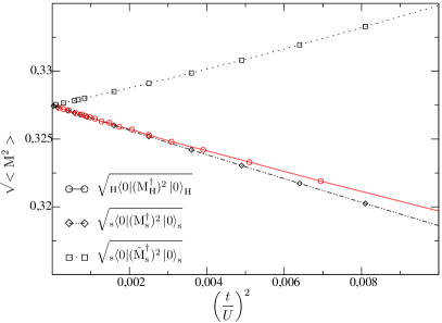
Figure 2: $t/U$ dependence of the staggered magnetization $M^{\dagger}_{2,{\rm s}}$, $M^{\dagger}_{2,{\rm H}}$ and $\tilde{M}_{2,{\rm s}}$ for a $2\times 4$ lattice.

In Fig. 2 we show results for $M^{\dagger}_{2,{\rm s}}$, $M^{\dagger}_{2,{\rm H}}$ and $\tilde{M}^{\dagger}_{2,{\rm s}}$ for a $2\times 4$ system. The full curve (circles) shows results for exact diagonalization of the Hubbard model, $M^{\dagger}_{2,{\rm H}}$,which should be considered as the reference data. One can see that $M^{\dagger}_{2,{\rm H}}$ is a decreasing function of $t/U$ at small $t/U$, as expected on physical grounds and as found in previous exact diagonalizations Fano and series expansion Shi . The dot-dashed curve (rhombuses) shows the result for $M^{\dagger}_{2,\rm s}$. While there is a quantitative difference between the two results, one finds that the two sets of data share the same slope, as $(t/U)^{2}\rightarrow 0$ and that their difference (not shown) scales as $(t/U)^{4}$ for small $t/U$. The dashed curve (squares) shows the $t/U$ dependence of the magnetic moment calculated from $\tilde{M}^{\dagger}_{2,{\rm s}}$ and $|0\rangle_{\rm s}$. Contrary to the exact result for $M^{\dagger}_{2,{\rm H}}$ and the SO result $M^{\dagger}_{2,{\rm s}}$, $\tilde{M}^{\dagger}_{2,{\rm s}}$ increases with (small) $t/U$, and never has the correct limiting small $t/U$ behavior. Simply calculating the staggered magnetic moment, as defined in a Heisenberg model, is therefore qualitatively incorrect when the low-energy Hamiltonian includes higher order corrections in $t/U$. On the contrary, when the correct SO operator $M^{\dagger}_{2,{\rm s}}$ is used, the result is not only qualitatively correct, but the difference between the exact Hubbard result and the SO result is less than $1\%$ for $t/U=0.1$. This suggests that $(4t/U)^{4}=.026$, with $4t$ the half-bandwidth, gives an estimate of the error on the staggered moment in the SO theory. Since the mapping between the Hubbard model and the effective theory is not size dependent, we expect this accuracy estimate to roughly apply in the thermodynamic limit.

III.2 Thermodynamic Limit: Spin Wave Calculation

As, in the absence of boundary effects, $M^{\dagger}_{\rm s}$ and $\tilde{M}^{\dagger}_{\rm s}$ differ only by a multiplicative factor (see Eq. (22) ), one can estimate the effect of this factor in the thermodynamic limit within a spin wave approximation. In this case, the spins operators are written in terms of their bosonic excitations through a Holstein Primakoff Holstein ; Kittel $1/S$ expansion of this bi-partite Néel ordered lattice:

Sublattice a Sublattice b

$$\left\{\begin{tabular}[]{ccl}$S_{i}^{z}$&$=$&$S-a_{i}^{\dagger}a_{i}$\\ $S_{i}^{+}$&$=$&$\sqrt{2S}[a_{i}\!+\!O(S^{-1})]$\\ $S_{i}^{-}$&$=$&$\sqrt{2S}[a_{i}^{{\dagger}}\!+\!O(S^{-1})]$\end{tabular}\right.$$

(25)

Transforming $H_{\rm s}$ in Eq. (11) in reciprocal space, one obtains to order $S$

$$H\,=\,H_{0}\,+\,\sum_{\vec{k}}A_{\vec{k}}\left(a_{\vec{k}}^{{\dagger}}a_{\vec{k}}\,+\,b_{\vec{k}}^{{\dagger}}b_{\vec{k}}\right)\,+\,B_{\vec{k}}\left(a_{\vec{k}}^{{\dagger}}b_{\vec{k}}^{{\dagger}}\,+\,a_{\vec{k}}b_{\vec{k}}\right),$$ (26)

where:

$$\left\{\begin{array}[]{ccl}A_{\vec{k}}&=&\displaystyle 4S(J_{1}-J_{2}-J_{3}-J_{c}S^{2}\,+\,(J_{2}-J_{c}S^{2})\nu_{\vec{k}}\\ &&\displaystyle+J_{3}\tau_{\vec{k}})\;\;\;,\\ B_{\vec{k}}&=&4S(J_{1}-J_{c}S^{2})\mu_{\vec{k}}\;\;\;,\\ H_{0}&=&-4NS^{2}(J_{1}-J_{2}-J_{3}-{\mathchoice{\dfrac{1}{2}}{\dfrac{1}{2}}{\frac{1}{2}}{\frac{1}{2}}}J_{c}S^{2})\end{array}\right.\;\;\;,$$ (27)

and

$$\left\{\begin{array}[]{ccl}\mu_{\vec{k}}&=&{\mathchoice{\dfrac{1}{2}}{\dfrac{1}{2}}{\frac{1}{2}}{\frac{1}{2}}}(\cos(k_{x})\,+\,\cos(k_{y}))\;\;\;,\\ \nu_{\vec{k}}&=&\cos(k_{x})\cos(k_{y})\;\;\;,\\ \tau_{\vec{k}}&=&{\mathchoice{\dfrac{1}{2}}{\dfrac{1}{2}}{\frac{1}{2}}{\frac{1}{2}}}(\cos(2k_{x})\,+\,\cos(2k_{y}))\;\;\;.\end{array}\right.$$ (28)

Defining

$$\epsilon_{\vec{k}}=\sqrt{A_{\vec{k}}^{2}-B_{\vec{k}}^{2}}\;\;\;,$$ (29)

we obtain the standard result Kittel

$$\langle\tilde{M}_{\rm s}^{{\dagger}}\rangle=S-\frac{1}{N}\sum_{\vec{k}}\left(\frac{A_{\vec{k}}}{\epsilon_{\vec{k}}}-\frac{1}{2}\right)\;\;\;.$$ (30)

We show in Fig. 3 the results for $\langle M^{\dagger}_{\rm s}\rangle$ and $\langle\tilde{M}^{\dagger}_{\rm s}\rangle$ calculated to order $1/S$ in the Holstein-Primakoff formulation of the Hamiltonian $H_{\rm s}$ in Eq. (11). The data show qualitatively the same behaviour as for the exact diagonalization (see Fig. 2): a positive trend at small $t/U$ for the moment $\tilde{M}_{\rm s}^{\dagger}$ of the SO model and a negative trend for the transformed moment $M_{\rm s}^{\dagger}$. Even though the ring exchange term is of order $S^{2}$ larger than the bilinear exchange terms, a calculation that would keep boson operators beyond quadratic order is apparently not required to get the correct qualitative trend of $M_{\rm s}^{\dagger}$ vs $t/U$.

Figure 3: $(t/U)$ dependence of $\langle M^{\dagger}_{\rm s}\rangle$ and $\langle\tilde{M}^{\dagger}_{\rm s}\rangle$ in a Holstein-Primakoff calculation of $H_{\rm S}$ to order $1/S$.

These results have several immediate consequences. We conclude that the increase of the Néel order parameter in the presence of ring-exchange  Lorenzana ; Honda ; Lauchli ; Honda-chain ; Katanin is due to the use of $\tilde{M}_{\rm s}^{\dagger}$, which neglects the renormalization factor $(1-2zt^{2}/U^{2})$ coming from charge quantum fluctuations. Further, we note that this renormalization factor is, to order $(t/U)^{2}$, identical to that reducing the spin-density wave amplitude in a Hartree-Fock solution of the Hubbard model Schrieffer-RPA .

We note here that it should not be construed that all quantities measuring the strength of the magnetic correlations need to be a monotonously decreasing function of $t/U$. For example, when considering the three-dimensional Hubbard model, where the Néel temperature $T_{\rm N}$ is nonzero, one finds that $T_{\rm N}/J=0.9575$ in the Heisenberg limit Staudt , where $J=4t^{2}/U$ is the nearest-neighbor Heisenberg exchange. Normalizing $T_{\rm N}$ by the scale $t$, we have $T_{\rm N}/t=3.83(t/U)$ in the Heisenberg limit Staudt ; Note_finite_T . Hence $T_{\rm N}/t$ is a non-monotonous function of $t/U$, first increasing as $U$ decreases from the Heisenberg limit, and then decreasing as the weak-coupling limit $t/U\gg 1$ is approached. However, this behavior comes the fact $T_{\rm N}/t$ is controlled by the spin stiffness which scales with $t/U$ in the opposite manner to the zero temperature order parameter, in the strong coupling limit. The spin stiffness is controlled by $J$ but the magnitude of the antiferromagnetic order parameter is not, as can be seen trivially in the Heisenberg limit where it is independent of $J$. More to the point is the observation that even for a relatively large $U/t=10$, $T_{\rm N}/t$ is already 25$\%$ below the Néel temperature that would be predicted by the Heisenberg model Staudt . Here, the charge fluctuations lower $T_{\rm Neel}$ of the Hubbard model below that of the corresponding limiting Heisenberg model. In the context of the work presented here, it would seem possible that a numerical calculation on a three-dimensional effective spin-only Hamiltonian to order $t(t/U)^{3}$ that neglects charge renormalization would give a Néel temperature that actually increases even faster than the Heisenberg $T_{\rm N}/t=3.83(t/U)$ and definitely faster than $T_{\rm N}$, obtained numerically for the Hubbard model.

IV Conclusion

We have shown that transforming the Hubbard model into an effective spin only theory leads, for $t/U$ away from the $t/U=0$ Heisenberg limit, to a new source of quantum fluctuations that reduces the staggered magnetization. Indeed, short-range charge fluctuations renormalize the order parameter by a factor $[1-2z(t/U)^{2}]$, depending on $t/U$, which is independent of the spin-only quantum fluctuations. This factor insures that increasing the charge mobility reduces the overall stability of the magnetic phase at $t/U>0$. This is despite the decrease in long range zero-point spin fluctuations which, when taken alone, suggests that the antiferromagnetic order parameter should become larger as $t/U$ increases from the Heisenberg limit. It would be interesting to find out whether this separation of charge and spin fluctuations is maintained to higher order in the perturbation scheme.

As a quantitative guide for the validity of the strong-coupling expansion, we also checked on small clusters that the difference between the result from the Hubbard model and that from the spin-only theory is of order $(4t/U)^{4}$ where the power 4 is the first power that is neglected in the derivation of the low-energy theory. We also showed that even though the ring exchange term is of order $S^{2}$ larger than the bilinear exchange terms, a calculation that would keep Holstein-Primakoff boson operators beyond quadratic order is apparently not required to get the correct qualitative trend of $M_{\rm s}^{\dagger}$ vs $t/U$.

Finally, note that charge fluctuations should also lead to amplitude renormalization factors for magnetic order at other wave vectors or for other order parameters such as dimerization. Renormalization factors for other effective models, such as the spin model coming from the three band model of the CuO₂ plane, and models that include second, $t^{\prime}$, and third, $t^{\prime\prime}$, nearest-neighbor hopping terms DGHT-2 , are also open problems.

V Acknowledgements

We thank G. Albinet, C. Bény, E. Dagotto, F. Delduc, S. Girvin, M. Jarrell, C. L’Huillier, A. Läuchli, J. Lorenzana, A. MacDonald, A. del Maestro, L. Raymond, M. Rice, R. Scalettar, D. Sénéchal and S. Sorella for useful discussions. Partial support for this work was provided by NSERC of Canada and the Canada Research Chair Program (Tier I) (M.G. and A.T.), Research Corporation and the Province of Ontario (M.G.), FQRNT Québec (A.T.) and a Canada$-$France travel grant from the French Embassy in Canada (M.G.and P.H.). M.G. and A.T. acknowledge support from the Canadian Institute for Advanced research.

Appendix A Derivation of the Spin Hamiltonian

Eq. (II.1) gives the expression for the third order expansion of the Hubbard model in terms of $T_{m}$ operators. Eqs. (9) and (10) introduce the mapping between the spin $S=1/2$ operator Hilbert space and the singly occupied subspace of the Hubbard model. In this mapping the calculation of the trace represents a somewhat subtle part because of the anticommutation relations between the different fermionic operators. As an example we derive the complete expression of the spin Hamiltonian to the first non zero order. We start with:

$$H^{(2)}\,=\,-{\mathchoice{\dfrac{1}{U}}{\dfrac{1}{U}}{\frac{1}{U}}{\frac{1}{U}}}\,T^{(2)}(-1,1),$$ (31)

that is:

$$H^{(2)} = {\mathchoice{\dfrac{t^{2}}{U}}{\dfrac{t^{2}}{U}}{\frac{t^{2}}{U}}{\frac{t^{2}}{U}}}\sum_{i_{1},i_{2},j_{1},j_{2}}\left(h_{i_{2},\bar{\sigma_{2}}}c_{i_{2},{\sigma_{2}}}^{{\dagger}}c_{j_{2},{\sigma_{2}}}n_{j_{2},\bar{\sigma_{2}}}\right)$$ (32)

$$\otimes\left(n_{i_{1},\bar{\sigma_{1}}}c_{i_{1},{\sigma_{1}}}^{{\dagger}}c_{j_{1},{\sigma_{1}}}h_{j_{1},\bar{\sigma_{1}}}\right).$$

Since we work in the singly occupied subspace ($\langle V\rangle=0$), the two electronic processes that first increase ($T_{1}$) and then decrease ($T_{-1}$) the number of doubly occupied sites have to be performed between the same 2 sites, which implies for Eq. (32) that:

$$\left\{\begin{tabular}[]{ccc}$j_{2}$&=&$i_{1}$\\ $i_{2}$&=&$j_{1}$\end{tabular}\right.$$ (33)

Defining the fermionic orbitals as:

$$\left|\underbrace{n_{1\uparrow},n_{1\downarrow}}_{1^{st}\,Site},\,\underbrace{n_{2\uparrow},n_{2\downarrow}}_{2^{nd}\,Site},\,\cdots,\,\underbrace{n_{N\uparrow},n_{N\downarrow}}_{N^{th}\,Site}\right\rangle\;\;\;.$$ (34)

For example, we have for two sites:

$$\left\{\begin{array}[]{ccccrcr}c_{1,\uparrow}\left|\uparrow,\uparrow\right\rangle&\equiv&c_{1,\uparrow}\left|1,0,1,0\right\rangle&=&\left|0,0,1,0\right\rangle&\equiv&\left|0,\uparrow\right\rangle\\ c_{2,\uparrow}\left|\uparrow,\uparrow\downarrow\right\rangle&\equiv&c_{2,\uparrow}\left|1,0,1,1\right\rangle&=&-\left|1,0,0,1\right\rangle&\equiv&-\left|\uparrow,\downarrow\right\rangle\\ c_{2,\downarrow}\left|\uparrow,\uparrow\downarrow\right\rangle&\equiv&c_{2,\downarrow}\left|1,0,1,1\right\rangle&=&\left|1,0,1,0\right\rangle&\equiv&\left|\uparrow,\uparrow\right\rangle\end{array}\right.,$$ (35)

the minus sign coming from the odd number of occupied fermionic orbitals occuring before the one specified by $c_{i,\sigma}$ or $c_{i,\sigma}^{{\dagger}}$. We use now the $\uparrow,\downarrow$ notation for simplicity, but it is important to notice that it represents fermionic orbital occupancy. The symbol $\left|0\right\rangle$ represents a site that is empty for both its orbitals $\uparrow$ and $\downarrow$. It follows that:

$$\left\{\begin{array}[]{ccc}T_{1}\left|\downarrow,\uparrow\right\rangle&=&-t\left|0,\downarrow\uparrow\right\rangle\,-\,t\left|\downarrow\uparrow,0\right\rangle\\ T_{1}\left|\uparrow,\downarrow\right\rangle&=&t\left|0,\downarrow\uparrow\right\rangle\,+\,t\left|\downarrow\uparrow,0\right\rangle\end{array}\right.,$$ (36)

$$\left\{\begin{array}[]{ccc}T_{-1}\left|0,\downarrow\uparrow\right\rangle&=&-t\left|\downarrow,\uparrow\right\rangle\,+\,t\left|\uparrow,\downarrow\right\rangle\\ T_{-1}\left|\uparrow\downarrow,0\right\rangle&=&-t\left|\downarrow,\uparrow\right\rangle\,+\,t\left|\uparrow,\downarrow\right\rangle\end{array}\right.,$$ (37)

and finally:

$$\left\{\begin{array}[]{ccc}T_{-1}T_{1}\left|\uparrow,\downarrow\right\rangle&=&2t^{2}\left\{\left|\uparrow,\downarrow\right\rangle\,-\,\left|\downarrow,\uparrow\right\rangle\right\}\\ T_{-1}T_{1}\left|\downarrow,\uparrow\right\rangle&=&-2t^{2}\left\{\left|\uparrow,\downarrow\right\rangle\ -\left|\downarrow,\uparrow\right\rangle\right\}\end{array}\right.\;\;\;.$$ (38)

We can then rewrite (32) as:

$$H^{(2)}\,=\,-{\mathchoice{\dfrac{t^{2}}{U}}{\dfrac{t^{2}}{U}}{\frac{t^{2}}{U}}{\frac{t^{2}}{U}}}\left(\left|\uparrow,\downarrow\right\rangle\ -\left|\downarrow,\uparrow\right\rangle\right)\left(\left\langle\uparrow,\downarrow\right|\ -\left\langle\downarrow,\uparrow\right|\right)$$ (39)

This form makes it easier to calculate the trace in (10) and gives:

$${\rm Tr}(\sigma_{1}^{x}\sigma_{2}^{x}H^{(2)})\,=\,-2{\mathchoice{\dfrac{t^{2}}{U}}{\dfrac{t^{2}}{U}}{\frac{t^{2}}{U}}{\frac{t^{2}}{U}}}$$ (40)

$${\rm Tr}(\sigma_{1}^{y}\sigma_{2}^{y}H^{(2)})\,=\,-2{\mathchoice{\dfrac{t^{2}}{U}}{\dfrac{t^{2}}{U}}{\frac{t^{2}}{U}}{\frac{t^{2}}{U}}}$$ (41)

$${\rm Tr}(\sigma_{1}^{z}\sigma_{2}^{z}H^{(2)})\,=\,-2{\mathchoice{\dfrac{t^{2}}{U}}{\dfrac{t^{2}}{U}}{\frac{t^{2}}{U}}{\frac{t^{2}}{U}}}$$ (42)

$${\rm Tr}(\sigma_{1}^{0}\sigma_{2}^{0}H^{(2)})\,=\,2{\mathchoice{\dfrac{t^{2}}{U}}{\dfrac{t^{2}}{U}}{\frac{t^{2}}{U}}{\frac{t^{2}}{U}}}$$ (43)

so that:

$$H_{\rm s}^{(2)}\,=\,-{\mathchoice{\dfrac{t^{2}}{U}}{\dfrac{t^{2}}{U}}{\frac{t^{2}}{U}}{\frac{t^{2}}{U}}}\sum_{<i,j>}\left(1-\bf{\sigma_{i}}\cdot\bf{\sigma_{j}}\right)\;\;\;,$$ (44)

or

$$H_{\rm s}^{(2)}\,=\,-{\mathchoice{\dfrac{4t^{2}}{U}}{\dfrac{4t^{2}}{U}}{\frac{4t^{2}}{U}}{\frac{4t^{2}}{U}}}\sum_{<i,j>}\left({\mathchoice{\dfrac{1}{4}}{\dfrac{1}{4}}{\frac{1}{4}}{\frac{1}{4}}}-\bf{S_{i}}\cdot\bf{S_{j}}\right)\;\;\;,$$ (45)

recovering the well known result of the nearest neighbor interaction coupling constant $J_{1}$:

$$J_{1}\,=\,{\mathchoice{\dfrac{4t^{2}}{U}}{\dfrac{4t^{2}}{U}}{\frac{4t^{2}}{U}}{\frac{4t^{2}}{U}}}$$ (46)

The same method can be applied to calculate the expression of the spin Hamiltonian up to order $t(t/U)^{3}$. As in Ref. MacDonald, , we used a program for the general construction of $H_{s}^{(k)}$ for $k\geq 4$. To order $k=4$, this leads to Eq. (11).

$$H_{\rm s}^{(4)} = J_{1}\!\!\sum_{<i,j>}{\bf S}_{i}\cdot{\bf S}_{j}\,+\,J_{2}\!\!\sum_{<i,j_{2}>}{\bf S}_{i}\cdot{\bf S}_{j_{2}}\,+\,J_{3}\!\!\sum_{<i,j_{3}>}{\bf S}_{i}\cdot{\bf S}_{j_{3}}$$ (47)

$$+ J_{c}\!\!\!\!\sum_{<i,j,k,l>}[({\bf S}_{i}\cdot{\bf S}_{j})({\bf S}_{k}\cdot{\bf S}_{l})+({\bf S}_{i}\cdot{\bf S}_{l})({\bf S}_{j}\,\cdot\,{\bf S}_{k})$$

$$\hskip 43.0pt\,-\,({\bf S}_{i}\cdot{\bf S}_{k})({\bf S}_{j}\,\cdot\,{\bf S}_{l})],$$

References

- (1)
- (2)
- (3) A.B. Harris and R.V. Lange, Phys. Rev. 157, 295, (1967).
- (4) A.H. MacDonald, S.M. Girvin, and D. Yoshioka, Phys. Rev. B 37, 9753 (1988); ibid, Phys. Rev. B 41, 2565 (1990); ibid, Phys. Rev. B 43, 6209 (1991).
- (5) A.L. Chernyshev et al., Phys. Rev. B 70, 235111, (2004).
- (6) M. Takahashi, J. Phys. C: Solid State Phys. 10, 1289 (1977)
- (7) A. W. Sandvik et al., Phys. Rev. Lett. 89, 247201 (2002).
- (8) A.M. Toader, J. P. Goff, M. Roger, N. Shannon, J. R. Stewart, and M. Enderle, Phys. Rev. Lett. 94, 197202 (2005) and references therein.
- (9) J. H. Van Vleck, Phys. Rev. 33, 467 (1929).
- (10) L. L. Foldy and S. A. Wouthuysen, Phys. Rev. 78, 29 (1950).
- (11) J. R. Schrieffer and P. A. Wolff, Phys. Rev. 149, 491 (1966).
- (12) H. Eskes et al., Phys. Rev. B 50, 17980 (1994),
- (13) A. Paramekanti, M. Randeria and N. Trivedi, Phys. Rev. Lett. 87, 217002 (2001); ibid, et al., Phys. Rev. B 70, 054504 (2004).
- (14) C. J. Hamer, W. Zheng, and R. R. P. Singh, Phys. Rev. B 68, 214408 (2003)
- (15) K. P. Schmidt and G. S. Uhrig, Phys. Rev. Lett. 90, 227204 (2003).
- (16) M.B.J. Meinders, H. Eskes, G.A. Sawatzky, Phys. Rev. B 48, 3916 (1993).
- (17) J. Lorenzana, J. Eroles, and S. Sorella, Phys. Rev. Lett. 83, 5122 (1999)
- (18) Y. Honda, Y. Kuramoto, and T. Watanabe, Phys. Rev. B 47, 11329 (1993).
- (19) A. Läuchli, G. Schmid, and M. Troyer, Phys. Rev. B 67, 100409 (2003);
- (20) Y. Honda and T. Horiguchi, cond-mat/0106426.
- (21) A.A. Katanin and A.P. Kampf, Phys. Rev. B 66, 100403 (2002).
- (22) J. R. Schrieffer, X. G. Wen, and S. C. Zhang, Phys. Rev. B 39, 11663 (1989). See Eq. (2.18) of that paper.
- (23) Z. P. Shi and R. R. P. Singh, Phys. Rev. B 52, 9620 (1995)
- (24) G. Fano, F. Ortolani, and A. Parola, Phys. Rev. B 46, 1048 (1992).
- (25) W.Stephan and P. Horsch, Int. J. Mod. Phys. B 6, 141 (1992).
-
(26)
The correct expression of the operator is
obtained from
which gives
The expectation value of this operator in a state with antiferromagnetic long-range order has a volume independent part that is identical to what would have been obtained by taking the square of the expectation value of the operator, as expected for a broken symmetry state. Note also, that to verify the spin commutation relations even to this low order in , one needs to unitary transform the commutator itself instead of taking the product of the spin operators that are operate in the spin-only low-energy subspace. - (27) C. Kittel, Quantum Theory of Solids, J. Wiley, New York (1986).
- (28) T. Holstein and H. Primakoff, Phys. Rev. 58, 1098 (1940)
- (29) R. Staudt, M. Dzierzawa, and A. Muramatsu, Eur. Phys. J. B 17, 411 (2000).
- (30) J.-Y. Delannoy et al, in preparation.
- (31) This means that in the large limit, at some finite temperature , antiferromagnetic correlations must increase with increasing , going from zero staggered magnetization to a finite value as one crosses the phase boundary. (See Ref. [Staudt, ]).