Self-organized Criticality and Absorbing States: Lessons from the Ising Model

Abstract

We investigate a suggested path to self-organized criticality. Originally, this path was devised to “generate criticality” in systems displaying an absorbing-state phase transition, but closer examination of the mechanism reveals that it can be used for any continuous phase transition. We used the Ising model as well as the Manna model to demonstrate how the finite-size scaling exponents depend on the tuning of driving and dissipation rates with system size. Our findings limit the explanatory power of the mechanism to non-universal critical behavior.

Self-organized criticality (SOC) refers to the spontaneous emergence of critical behavior in slowly driven dissipative systems Bak et al. (1987); Jensen (1998). Most models are defined on lattices with local particle numbers $z_{i}$ and thresholds $z_{i}^{c}$. They are driven discretely in time by increasing $z_{i}$ at randomly chosen positions $i$ until such an increase leads to $z_{i}>z_{i}^{c}$ somewhere in the system. Particles then topple to neighboring sites and can trigger avalanches of local redistribution propagating through the entire lattice. Dissipation typically takes place at the boundaries, where particles leave the system. When an avalanche has finished the model is driven again Jensen (1998). The resulting avalanche size distributions obey simple scaling.

In models displaying absorbing state (AS) phase transitions Hinrichsen (2000) a tuning parameter, such as the overall particle density, controls a transition between an inactive phase and a phase where activity in the system continues indefinitely.

From the first introduction of SOC in 1987 Bak et al. (1987), it was believed that SOC models manoeuver themselves to the critical density between similar inactive and active phases. Tang and Bak suggested in 1988 that the density of “lattice sites on which $z>z_{c}$ […] may be viewed as the order parameter for this critical phenomenon” Tang and Bak (1988). Such an identification of the activity with the order parameter implies a link to absorbing state phase transitions.

This link was formalized and made explicit about 10 years later Vespignani and Zapperi (1997); Dickman et al. (1998, 2000); Dickman (2002). Dickman et al. Dickman et al. (1998) introduced periodic boundaries to SOC systems, thereby turning them into AS models. Measuring the exponents characterizing the spreading of perturbations Vespignani et al. (2000); Chessa et al. (1998) or the roughness of the associated interface models Vespignani et al. (2000); Dickman et al. (2001), it has been observed that at the critical density the closed-model behavior resembles that of open SOC models Dickman et al. (1998); Christensen et al. (2004).

The resulting interpretation of SOC is obvious Dickman et al. (1998, 2000); Dickman (2002): Activity eventually leads to dissipation at the boundaries, which in turn reduces the particle density to below the critical value. Driving takes place whenever quiescence has been reached. SOC models therefore hover around the critical point, being pushed forth into the active state by driving and pushed back into the quiescent state by dissipation.

With this simple picture in mind one arrives at an equation of motion for the particle density $\zeta$ in the system Vespignani et al. (1998); Vespignani and Zapperi (1998)

$$\frac{d}{ds}\zeta(s)=h-\rho_{a}(s)\epsilon\ ,$$ (1)

where $s$ is the time, $h$ is the driving rate and $\epsilon$ is called the (bulk) dissipation rate. The activity $\rho_{a}$ is the order parameter, defined as the density of active sites, $z_{i}>z_{i}^{c}$, in the active phase. We will refer to this interpretation of SOC as “the AS approach”.

Clearly, the driving $h$ must be very slow compared to the dissipation $\rho_{a}\epsilon$. Otherwise particles would be added while the system is active, leading to a fluctuating activity rather than distinct avalanches. The proponents of the AS approach point out that $h$, $\epsilon$ and $h/\epsilon$ have to be tuned to zero in order to achieve the desired separation of timescales Vespignani and Zapperi (1997). While the definitions of SOC models typically restrict dissipation to boundary sites and result in diverging avalanche sizes in the thermodynamic limit, leading to appropriately vanishing $\epsilon(L)$ and $h(L)$, so far no statement has been made as to how the limiting behaviour is approached. But this turns out to be the all-important piece of information: The finite-size scaling (FSS) behavior, the only scaling available in SOC, depends entirely on the scaling of the driving and dissipation rates with system size. Choosing $h(L)$ and $\epsilon(L)$ freely, arbitrary scaling behavior is produced.

In the following the relation between the scaling of $h$ and $\epsilon$ and the resulting FSS is analyzed, using the two dimensional Ising model as an example. However, the analysis is generally applicable and works equally well for standard SOC models and their AS counterparts, which is confirmed by simulations of the Manna model Manna (1991); Dickman et al. (2001).

Translating Eq. (1) into magnetic language, $\zeta$ corresponds to the inverse temperature $\beta$ and the activity $\rho_{a}$ to the modulus of the magnetization density $|m|$. The parameters $h$ and $\epsilon$ become cooling and heating rates, so that the temperature $T$ is increased for large magnetizations and lowered otherwise,

$$\frac{d}{ds}\beta(s)=h-|m(s)|\epsilon\ .$$ (2)

The resulting model is an Ising model where the temperature is dynamically adapted according to the equation of motion (2). Therefore, the configurations are not sampled with Boltzmann-weight and the resulting “dynamical ensemble” is not canonical. However, by multiplying (2) by a small pre-factor, corresponding to rescaling the time, the distribution of temperatures can be made arbitrarily narrow. For the sake of the following analysis, it is assumed that this “dynamical Ising model” is well characterized by a single effective (reduced) temperature, $t_{\text{eff}}$.

For the FSS analysis presented below we choose the approach of $h,\epsilon\to 0$ to leading order as

$$h=h_{0}L^{-\omega}\ \text{and}\ \epsilon=\epsilon_{0}L^{-\kappa},$$ (3)

where $\omega,\kappa>0$. In the stationary state, $\left\langle\frac{d}{ds}\beta\right\rangle=0$, (2) yields $\left\langle|m|\right\rangle=(h_{0}/\epsilon_{0})L^{\kappa-\omega}$ with $\left\langle\right\rangle$ denoting the average over the dynamical ensemble introduced above. Clearly one must choose $\omega>\kappa$. To attain the prescribed $\left\langle|m|\right\rangle(L)$ the system settles at the effective (reduced) temperature $\left\langle T-T_{c}\right\rangle/T_{c}\equiv t_{\text{eff}}(L)\propto L^{-1/\mu}$ to leading order, see Fig. 1. Via $t_{\text{eff}}(L)$ all thermodynamic quantities depend only on $L$, which can be mistaken for standard FSS at temperature $T=T_{c}$. For the study of SOC models it is vital to understand the difference because SOC systems are always critical, wherefore FSS is the only scaling available.

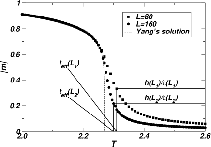
Figure 1: Finite size behaviour for the magnetisation $|m|$ versus the temperature $T$ in the regular, 2D-Ising model for $L_{1}=80$ (squares) and $L_{2}=160$ (circles). The dashed line shows Yang’s solution Yang (1952). In the dynamical Ising model, the cooling and heating rates, $h(L)$ and $\epsilon(L)$ prescribe the magnetisation $|m(L)|=h(L)/\epsilon(L)\propto L^{\kappa-\omega}$, indicated by horizontal lines. The system is forced to move to an effective temperature $t_{\text{eff}}(L)$, indicated by arrows.

Around the critical point of a continuous phase transition, the singular part of the free energy leads to a simple scaling behavior of the magnetization density Privman et al. (1991),

$$\left\langle|m|\right\rangle=-k_{h}L^{-\beta/\nu}Y^{\prime}(k_{t}tL^{1/\nu}),$$ (4)

where $t$ is the reduced temperature, negative in the low temperature phase (LTP) and positive in the high temperature phase (HTP). $k_{h}$ and $k_{t}$ are metric factors, and $Y^{\prime}(x)$ is a universal scaling function, which becomes dependent on the boundary conditions and the geometry of the system in the limit of small arguments, case (5b) below. There are three qualitatively different (asymptotic) regimes

$$Y^{\prime}(x)\to \propto|x|^{\beta} x\to-\infty$$ for (5a)

$$Y^{\prime}(x)\to x\to 0$$ const. for (5b)

$$Y^{\prime}(x)\to \propto x^{-\gamma/2} x\to\infty$$ for , (5c)

where in the Ising model $\gamma=\nu d-2\beta$.

The first line describes the asymptotic behavior of the magnetization in the LTP, the second line represents FSS, and the third line describes the HTP.

Setting $\left\langle|m|\right\rangle\propto L^{\kappa-\omega}$, the different regimes of (5c) are accessed by three qualitatively different choices of $\kappa-\omega$, that is speeds at which $\left\langle|m|\right\rangle$ approaches zero:

• $\kappa-\omega>-\beta/\nu$ (“too slow”): In this case the magnetization approaches $0$ slower than in a standard Ising model kept at temperature $T=T_{c}$ as the system size increases, so that $Y^{\prime}(k_{t}t_{\text{eff}}(L)L^{1/\nu})\propto L^{\kappa-\omega+\beta/\nu}$ is divergent in $L$. The only way to obtain a divergent $Y^{\prime}(x)$ is via (5a), which requires a negatively divergent argument $x\to-\infty$. The effective temperature is therefore negative and scales like $|t_{\text{eff}}(L)|^{\beta}\propto L^{\kappa-\omega}$. Using $t_{\text{eff}}(L)\propto L^{-1/\mu}$ leads to

  $$\mu=\beta/(\omega-\kappa)>\nu\ .$$ (6)

  This implies that $t_{\text{eff}}(L)$ finally leaves the FSS region, whose width scales like $L^{-1/\nu}$, toward the LTP.

• $\kappa-\omega=-\beta/\nu$ (“correct”): In this case $Y^{\prime}(x)$ remains constant, so that its argument either remains constant or vanishes, according to (5b). Thus $t_{\text{eff}}(L)$ decays at least as fast as $L^{-1/\nu}$, i.e. $\mu\leq\nu$. To the order considered here the equality applies.

• $\kappa-\omega<-\beta/\nu$ (“too fast”): $Y^{\prime}(x)$ vanishes, following (5c). For $Y^{\prime}(k_{t}t_{\text{eff}}(L)L^{1/\nu})\propto L^{\kappa-\omega+\beta/\nu}$ and $t_{\text{eff}}\propto L^{-1/\mu}$ this implies

  $$\mu=\frac{\gamma\nu}{2\nu(\kappa-\omega+\beta/\nu)+\gamma}>\nu\ ,$$ (7)

  provided that the denominator of Eq. (7) is positive. Hence the model leaves the FSS region toward the HTP. The special case of negative $\mu$, implying divergent effective temperature, will be ignored.

Crucially, only for $\kappa-\omega=-\beta/\nu$ (case 2)) does the model remain in the FSS region. To achieve this, $h/\epsilon$ must be tuned exactly in the way the order parameter scales in a system displaying standard FSS, $\left\langle|m|\right\rangle\propto L^{-\beta/\nu}$ while fixed at the critical temperature. In all other cases the scaling of the effective temperature eventually drives the model out of the FSS region: $\xi/L$ vanishes in the thermodynamic limit. Nevertheless, $\left\langle T\right\rangle$ converges to $T_{c}$, so that the correlation length

$$\xi\propto L^{\nu/\mu}$$ (8)

diverges. With this scaling of $\xi$ all observables will show standard finite-size scaling with $\nu$ replaced by $\mu$ .

To illustrate the above analysis we performed simulations of an Ising model with dynamics as described: Using Metropolis updating, the absolute magnetization density is calculated after each scan over the lattice. According to (2) a new temperature is then calculated to be used in the next sweep, $\dot{T}=-h+\left\langle|m|\right\rangle\epsilon$. Starting from $T=2.27$, systems of size $L=40,80...640$ were updated at least $10^{6}$ times as transient and at least another $10^{6}$ times for statistics.

Our numerical simulations fully confirm the above analysis: We observe the standard FSS exponents with $\nu$ replaced by $\mu$ for any reasonable choice of $\kappa-\omega$. The new scaling exponent $\mu$ (and $T_{c}$) can be determined from $\left\langle T\right\rangle-T_{c}\propto L^{-1/\mu}$. Using it in an FSS analysis allows us to identify all standard critical exponents. Even without the knowledge of $\mu$ three measurements, say $\alpha/\mu$, $\beta/\mu$ and $\gamma/\mu$, are sufficient to determine all exponents using standard scaling laws. This seems to defy common sense, since the exponents are determined without referring to $T_{c}$, making it seemingly very attractive for investigations of continuous phase transitions. However, standard methods, such as FSS or analysis of the critical behavior at $\xi\ll L$, are much more reliable and efficient: Not only is the above identification of $t_{\text{eff}}$ with the reduced temperature questionable. More importantly, almost any choice of the scaling of $h$ and $\epsilon$ leads to vanishing $\xi/L$. One therefore simulates effectively independent patches of a lattice in a way that FSS effects remain important.

For two reasons the method is very sensitive to the choice of $\epsilon_{0}$ and $h_{0}$ in Eq. (3) : Firstly, the amplitudes of the fluctuations in the effective temperature depend directly on $h$ and $\epsilon$; choosing $h_{0}$ and $\epsilon_{0}$ too large, the system destabilizes. One can estimate these fluctuations by analyzing (2) and derive a lower bound for $\kappa,\omega$. Secondly, if $h$ and $\epsilon$ are too small and initially place the system close to $T_{c}$, the scaling function reaches its asymptotic behavior (generally (5c) or (5a)) only for very large system sizes.

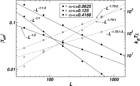
Figure 2: The scaling of the effective temperature $t_{\text{eff}}$ (filled symbols, full lines) and the susceptibility $\chi$ (open symbols, dashed lines) in the Ising model for different choices of the exponent $\kappa$ and $\omega=1$. The symbols are numerical simulations, the lines show the slopes expected from theory.

Fig. 2 shows the scaling of the effective temperature for the three qualitatively different choices of the driving exponents discussed above. The values of $\mu$ and $\gamma$ derived from these data confirm the calculations. Depending on the choice of $\kappa-\omega$, the value of $\mu$ immediately determines either $\beta$, Eq. (6), or $\gamma$, Eq. (7). The FSS of specific heat and susceptibility produces the expected values of $\alpha/\mu$ and $\gamma/\mu$.

Since our interest in the AS approach is due to its proposed role as an explanation for SOC, we repeated the analysis for a variant of the one-dimensional Abelian Manna model Manna (1991). This sandpile-like model has been used to exemplify the link between SOC and AS Dickman et al. (1998, 2000); Vespignani et al. (2000). It is driven in the bulk and implements bulk dissipation Barrat et al. (1999), as suggested by (1). While the key equation (4) has been confirmed Dickman et al. (2001), the Manna model is neither as well understood nor as well-behaved as the Ising model. Unlike in the Ising model, the Manna model can get stuck when hitting an inactive state. This complicates the analysis especially for the third case discussed above. Nonetheless the effective particle density $\left\langle\zeta\right\rangle$ is certainly a function of $h$ and $\epsilon$ and therefore depends on their scaling with all the consequences laid out above. Indeed, the numerics agrees fairly well with the theoretical predictions. Most crucially, the activity as well as the scaling of the avalanche size distribution show a clear, immediate dependence on the choice of the two exponents $\omega$ and $\kappa$.

One should note that introducing bulk-drive and -dissipation to SOC models does not result in a full correspondence to AS models. Firstly, there are important observables in SOC lacking a counterpart in AS and vice versa. For example, there is no obvious definition of the avalanche size in the active phase of an AS model. Similarly, the definition of the SOC-activity is somewhat arbitrary in Abelian models Dhar (1999), due to the lack of a unique microscopic timescale, which is needed when taking temporal averages or measuring rates. Secondly, for AS models Eq. (4) contains the asymptotic conditional activity, while in bulk-driven SOC models, such as the Manna model presented above, the instantaneous activity enters into the equation of motion (1).

The present study shows that the proposed explanation of SOC as “self-organized” AS criticality Dickman et al. (1998, 2000); Dickman (2002) implies non-universal scaling behavior dependent on $\kappa-\omega$. Universal, that is dissipation- and driving-independent, scaling behavior cannot be achieved with the AS approach. The question whether SOC models have universal features is very important. Universality is a main justification for studying simple models and for disregarding the details of the physical processes they describe.

Despite the importance of this issue, it is still unclear whether SOC systems can be grouped into universality classes; in fact, exponents can change due to small changes in the update rules (e.g. Malthe-Sørenssen (1999); Olami et al. (1992)), and SOC is notorious for its wide variety of critical exponents. Accepting the AS approach this would be a consequence of implicitly setting the scaling of external drive and dissipation by the dynamical rules of the different models.

However, there is also strong evidence in favor of universality in SOC. Many changes of the detailed dynamics do not affect the critical behavior Pruessner and Jensen (2003); Bengrine et al. (1999a, b); Zhang (1997). Moreover, the ratio $\xi/L$ appears to remain constant in direct measurements of some models Peters (2004) so that the “correct” FSS exponents are observed, which is in stark contrast to (8).

At first sight, the observation of the same exponents in SOC and AS models (such as Chessa et al. (1998); Vespignani et al. (2000); Christensen et al. (2004)) seems to support the case for the AS approach. But our analysis shows that the opposite is true: If the AS approach was determining the behaviour of SOC models, it would almost certainly (apart from case 2)) produce exponents which differ from those observed in their AS counterparts. Barring coincidence, observations supporting universality in SOC must therefore be taken as strong evidence against the AS approach explaining the critical behavior of SOC models.

We have calculated the FSS behaviour of a system approaching its critical point through a feedback mechanism between order parameter and tuning parameter. While scale-free distributions of responses such as those observed in the case of rainfall Peters et al. (2002) or earthquakes Gutenberg and Richter (1944), can be produced by such a process, it only yields critical behavior strongly dependent on the detailed dynamical rules of SOC models. There would be no universality and robustness against small changes in the dynamical rules. While the AS mechanism in its present form may produce further insight into potentially non-universal critical phenomena as observed in field experiments, it fails to explain the apparent universality of SOC models.