Zero-Momentum Cyclotron Spin-Flip Mode in a Spin-Unpolarized Quantum Hall System

Abstract

We report on a study of the zero-momentum cyclotron spin-flip excitation in the ${\mbox{\scriptsize${\cal V}$}}\!=\!2$ quantum Hall regime. Using the excitonic representation the excitation energy is calculated up to the second order Coulomb corrections. A considerable negative exchange shift relative to the cyclotron gap is established for cyclotron spin-flip excitations in the the spin-unpolarized electronic system. Under these conditions this type of states presents the lowest-energy excitations. For a fixed filling factor (${\mbox{\scriptsize${\cal V}$}}\!=\!2$) the energy shift is independent of the magnetic field which is in agreement with recent experimental observations.

PACS numbers: 73.43.Lp, 78.66.Fd

1. It is well known that in a translationally invariant two-dimensional electron system Kohn’s theorem  ko61 prohibits coupling of a homogeneous external perturbation to collective excitations of the electrons. As a result, the energy of cyclotron excitations (CE) at zero-momentum has no contribution from Coulomb interaction and the dispersion of CE starts from the cyclotron gap. In addition to inter-Landau-levels cyclotron excitations [magnetoplasma (MP) mode] there are two other branches of collective excitations in the system of 2D-electrons: intra-Landau levels spin-flip (SF) excitations (spin-waves) and inter-Landau-levels combined cyclotron spin-flip excitations (CSFE’s). In the case of SF excitations, there exists Larmor’s theorem which forbids any contribution from Coulomb interaction to the excitation energy at zero-momentum in spin rotationally invariant systems (see, e.g., Ref. ka84, ). However, in contrast to the CE and SF excitations, there are no symmetry reasons for the absence of many-body corrections to the zero-momentum energy of CSFE’s. Moreover, it is well established now both theoretically and experimentally  pi92 that for the spin-polarized electron system (${\mbox{\footnotesize${\cal V}$}}\!=\!1$) the energy of cyclotron spin-flip excitations is strongly shifted to higher values relative to the cyclotron gap due to the exchange interaction. Therefore, the energy of combined cyclotron spin-flip excitations is a very convenient tool to probe many-body effects, for example, in the inelastic light scattering measurements performed at zero momentum. The sensitivity of CSFE energy at ${\bf q}=0$ to many-body effects strongly depends on the spin polarization of the electron system. For the spin-unpolarized electron system (${\mbox{\footnotesize${\cal V}$}}\!=\!2$), theory ka84 developed within the first order perturbation approach in terms of the parameter $r_{c}=E_{C}/\hbar\omega_{c}$ ($E_{C}$ is the characteristic Coulomb energy, $\omega_{c}$ is the cyclotron frequency) predicts a zero many-body contribution to the zero-momentum energy of CSFE. This result is in contradiction with recent experimental data. kul04 We show below that calculation of the CSFE zero-momentum energy of for the ${\mbox{\footnotesize${\cal V}$}}\!=\!2$ system performed to within the second order Coulomb corrections yields a considerable negative exchange shift relative to the cyclotron gap.

The studied system is characterized by exact quantum numbers $S$, $S_{z}$ and ${\bf q}$ and by a non-exact but ‘good’ quantum number $\delta n$ corresponding to the change of the single-electron energy $\hbar\omega_{c}\delta n$ with an excitation. The relevant excitations with ${\bf q}\!=\!0$ and $\delta n\!=\!1$ may be presented in the form ${\hat{K}}_{S,S_{z}}^{{\dagger}}|{\bf 0}\rangle$, where $|{\bf 0}\rangle$ is the ground state and ${\hat{K}}_{S,S_{z}}^{{\dagger}}$ are “raising” operators: $\!{\hat{K}}_{0,0}^{{\dagger}}\!\!=\!\!\sum_{np\sigma}\!{}\!\sqrt{n+1}c^{{\dagger}}_{n\!+\!1,p,\sigma}c_{n,p,\sigma},\;{\hat{K}}_{1,0}^{{\dagger}}\!\!=\!\!\sum_{np\sigma}\!{}\!\sqrt{n+1}\,(-1)^{\sigma}c^{{\dagger}}_{n\!+\!1,p,\sigma}c_{n,p,\sigma}\qquad\mbox{and}\qquad{\hat{K}}_{1,+/-}^{{\dagger}}=\sum_{np}\!{}\!\sqrt{n+1}c^{{\dagger}}_{n\!+\!1,p,\uparrow/\downarrow}c_{n,p,\downarrow/\uparrow}$, [$c_{n,p,\sigma}$ is the Fermi annihilation operator corresponding to the Landau-gauge state $(n,p)$ and spin index $\sigma\!\!=\!\uparrow,\!\downarrow$]. The commutators with the kinetic-energy operator ${\hat{H}}_{1}$ are $[{\hat{H}}_{1},{\hat{K}}_{S,S_{z}}^{{\dagger}}]\!\!\equiv\!\!\hbar\omega_{c}{\hat{K}}_{S,S_{z}}^{{\dagger}}$. (The total Hamiltonian is ${\hat{H}}_{\mbox{\scriptsize tot}}\!=\!{\hat{H}}_{1}\!+\!{\hat{H}}_{\mbox{\scriptsize int}}$, where ${\hat{H}}_{\mbox{\scriptsize int}}$ is the exact Coulomb-interaction Hamiltonian.) If $|{\bf 0}\rangle$ is unpolarized, we have ${\hat{\bf S}}^{2}{\hat{K}}_{S,S_{z}}^{{\dagger}}|{\bf 0}\rangle\!\!\equiv\!\!S(S\!+\!1){\hat{K}}_{S,S_{z}}^{{\dagger}}|{\bf 0}\rangle$, ${\hat{S}}_{z}{\hat{K}}_{S,S_{z}}^{{\dagger}}|{\bf 0}\rangle\!\!\equiv\!\!S_{z}{\hat{K}}_{S,S_{z}}^{{\dagger}}|{\bf 0}\rangle$ and besides get the identity $\langle{0}|{\hat{K}}_{S,S_{z}}[{\hat{H}}_{\mbox{\scriptsize int}},{\hat{K}}_{S,S_{z}}^{{\dagger}}]|{0}\rangle\!\equiv\!0$ ($|0\rangle$, to describe the zero’th order ground state). The latter determines the first-order Coulomb corrections vanishing both for the $S\!=\!0$ MP mode and for the $S\!=\!1$ triplet states corresponding to the combined spin-cyclotron excitation. At the same time $[{\hat{H}}_{\mbox{\scriptsize int}},{\hat{K}}_{0,0}^{{\dagger}}]\!\equiv\!0\,$ ko61 but $[{\hat{H}}_{\mbox{\scriptsize int}},{\hat{K}}_{1,S_{z}}^{{\dagger}}]\!\neq\!0$ which means that the MP mode indeed has no exchange energy calculated to any order in $r_{c}$, whereas the triplet states have the exchange correction even in terms of $r_{c}^{2}$.

The second-order correction, $\Delta E_{\mbox{\scriptsize SF}}\!\sim\!\hbar\omega_{c}r_{c}^{2}$, does not depend on the magnetic field since $E_{C}\!=\!\alpha e^{2}/\varepsilon l_{B}$. The renormalization factor, $\alpha$, is determined by the size-quantized wave function of electrons confined to the quantum well (QW). In the ideal 2D case $\alpha\!=\!1$. However, in experiments with comparatively wide QW’s we expect a well reduced value of $\alpha$. Our analytical calculation of the second order correction to the CSFE energy is performed in terms of $r_{c}$ assumed to be small.

All three triplet states have certainly the same exchange energy, and it is sufficient to calculate this, e.g., for the CSFE with $S\!=\!1$ and $S_{z}\!=\!-\!1$. The obtained result confirms experimental observations.

2. The most adequate approach to the integer-quantum-Hall calculations is based on the Excitonic Representation (ER) di02 ; dz83 technique (see also, e.g., Refs. di96, ). The latter means that instead of single-electron states belonging to a continuously degenerate Landau level (LL) we employ the exciton states ${\cal Q}_{ab\,{\bf q}}^{{\dagger}}|0\rangle$ as the basis set. Here $|0\rangle$ is the ground state found in the zero approximation in $r_{c}$ (it remains also the same even calculated within the framework of the mean field approach). The exciton creation operator is defined as  dz83 ; di02 ; di96 ; by87

$$\vspace{-2.mm}{\cal Q}_{ab\,{\bf q}}^{{\dagger}}=\frac{1}{\sqrt{N_{\phi}}}\sum_{p}\,e^{-iq_{x}p}b_{p+\frac{q_{y}}{2}}^{{\dagger}}\,a_{p-\frac{q_{y}}{2}}\,.$$

$N_{\phi}=A/2\pi l_{B}^{2}$ stands for the number of magnetic flux quanta, ${\bf q}\!=\!(q_{x},q_{y})$ is the 2D wave vector in units of $1/l_{B}$. Binary indexes $a$ and $b$ present both the LL number and spin index. [I.e. $a\!=\!(n_{a},\sigma_{a})$, and $a_{p}$ in Eq. (1) stands for the corresponding annihilation operator; when exploiting below the notation $a\!=\!n$ or $a\!=\!{\overline{n}}$ as sublevel indexes, this means that $a\!=\!(n,\uparrow)$ or $a\!=\!(n,\downarrow)$, respectively.] The annihilation exciton operator is ${\cal Q}_{ab\,{\bf q}}\!\equiv\!{\cal Q}_{ba\,-\!{\bf q}}^{{\dagger}}$. The commutation rules define a special Lie algebra: di02 ; di96 ; by87

$$\begin{array}[]{l}{}\!\!{}\!{}\!{}\!{}\!{}\!{}\!\left[{\cal Q}_{cd\,{\bf q}_{1}}^{{\dagger}},{\cal Q}_{ab\,{\bf q}_{2}}^{{\dagger}}\right]\!\equiv\!N_{\phi}^{-1/2}\left[e^{-i({\bf q}_{1}\!\times\!{\bf q}_{2})_{z}/2}\delta_{b,c}{\cal Q}_{ad\,{\bf q}_{1}\!+\!{\bf q}_{2}}^{{\dagger}}\right.\\ \qquad{}\qquad{}\quad{}-\!\left.e^{i({\bf q}_{1}\!\times\!{\bf q}_{2})_{z}/2}\delta_{a,d}{\cal Q}_{cb\,{\bf q}_{1}\!+\!{\bf q}_{2}}^{{\dagger}}\right],\end{array}$$

where $\delta_{a,b}\!=\!\delta_{n_{a},n_{b}}\delta_{\sigma_{a},\sigma_{b}}$ is the Kronecker symbol. In the ${\mbox{\footnotesize${\cal V}$}}\!=\!2$ case we get the following identity: $N_{\phi}^{-1/2}{\cal Q}_{aa\,{\bf q}}^{{\dagger}}|0\rangle\!\equiv\!\delta_{{\bf q},0}\left(\delta_{a,0}\!+\!\delta_{a,{\overline{0}}}\right)|0\rangle$.

The advantage of the exciton states lies in the fact that an essential part of the Coulomb interaction Hamiltonian may be diagonalized in this basis. In the perturbative approach the excitonically diagonalized part ${\hat{H}}_{\mbox{\scriptsize ED}}$ should be included into the unperturbed Hamiltonian ${\hat{H}}_{0}={\hat{H}}_{1}\!+\!{\hat{H}}_{\mbox{\scriptsize ED}}$ and only the off-diagonal part ${\hat{\cal H}}_{\mbox{\scriptsize int}}\!=\!{\hat{H}}_{\mbox{\scriptsize int}}\!-\!{\hat{H}}_{\mbox{\scriptsize ED}}$ is considered as a perturbation. di02 In the excitonic basis the LL degeneracy becomes well lifted because now there are Coulomb corrections (depending on the ${\bf q}$ modulus) to the energies of the basis states. It is useful to take into account that all terms of the relevant ${\hat{\cal H}}_{\mbox{\scriptsize int}}$ part may be presented in the form (cf. Ref. di02, )

$$\begin{array}[]{l}{}\!{}\!{}\!{}\!{\hat{\cal H}}_{\mbox{\scriptsize{int}}}={\displaystyle\frac{e^{2}}{2\varepsilon l_{B}}}\sum_{{\bf q},a,b,c,d}V({\bf q})\left[h_{n_{a}n_{b}}({\bf q})\delta_{\sigma_{a},\sigma_{b}}{{\cal Q}}_{ab{\bf q}}^{{\dagger}}\right]\\ {}\quad{}\qquad{}\qquad{}\qquad{}\qquad\times\!\left[h_{n_{c}n_{d}}(-{\bf q})\delta_{\sigma_{c},\sigma_{d}}{{\cal Q}}_{cd\,-\!{\bf q}}^{{\dagger}}\right].\end{array}\vspace{-1mm}$$

Here $2\pi V({\bf q})$ is the dimensionless 2D Fourier component of the averaged Coulomb potential (in the ideal 2D case $V\!=\!1/q$), and $h_{kn}({\bf q})=({k!}/{n!})^{1/2}e^{-q^{2}/4}(q_{-})^{n\!-\!k}L^{n\!-\!k}_{k}(q^{2}/2)$ are the ER “building-block” functions ($L_{k}^{n}$ is the Laguerre polynomial, $q_{\pm}=\mp\frac{i}{\sqrt{2}}(q_{x}\pm iq_{y})$; cf. also Ref. ka84, and Refs. di02, ; di96, ). The functions $h_{kn}$ satisfy the identity: $h_{kn}^{*}({\bf q})\!\equiv\!h_{nk}(-{\bf q})$.

At the ${\mbox{\footnotesize${\cal V}$}}\!=\!2$ filling the CSFE state calculated within the zero order in ${\hat{\cal H}}_{\mbox{\scriptsize int}}$ is simply $|SF\rangle{}\!=\!{\hat{Q}}_{{0}\overline{1}}^{{\dagger}}|0\rangle$ (the notation ${\hat{\cal Q}}_{ab\,{\bf 0}}^{{\dagger}}\!=\!{\hat{Q}}_{ab}^{{\dagger}}$ is employed). We thus have ${\hat{H}}_{\mbox{\scriptsize ED}}Q^{{\dagger}}_{{0}\overline{1}}|0\rangle\!=\!\langle 0|{\cal Q}_{ab\,{\bf q}}{\hat{\cal H}}_{\mbox{\scriptsize int}}Q^{{\dagger}}_{{0}\overline{1}}|0\rangle\!=\!0$ for any indexes ${\bf q}$ and $ab$ (one could check it directly using the ER approach; see also Ref. ka84, ). Action of ${\hat{\cal H}}_{\mbox{\scriptsize int}}$ on the $|SF\rangle$ state leads to two- and or even three-exciton states. Therefore the excitonic basis should be extended.

3. In principle, there are eight different kinds of possible two-exciton states at ${\mbox{\footnotesize${\cal V}$}}\!=\!2$. In our case the relevant ones are those corresponding to spin numbers $S_{z}\!=\!-1$ and $S\!=\!0$, namely: $|\nu,1\rangle\!=\!{\cal Q}_{0n_{2}\,-\!{\bf q}_{\nu}}^{{\dagger}}\!{\cal Q}_{0\overline{n}_{1}\,{\bf q}_{\nu}}^{{\dagger}}|0\rangle$, $|\nu,2\rangle\!=\!{\cal Q}_{\overline{0}\overline{n}_{2}\,-\!{\bf q}_{\nu}}^{{\dagger}}\!{\cal Q}_{0\overline{n}_{1}\,{\bf q}_{\nu}}^{{\dagger}}|0\rangle$, $|\nu,3\rangle\!=\!\frac{1}{2}{\cal Q}_{0n_{2}\,-\!{\bf q}_{\nu}}^{{\dagger}}\!{\cal Q}_{0n_{1}\,{\bf q}_{\nu}}^{{\dagger}}|0\rangle$, $|\nu,4\rangle\!=\!{\cal Q}_{0n_{2}\,-\!{\bf q}_{\nu}}^{{\dagger}}\!{\cal Q}_{\overline{0}\overline{n}_{1}\,{\bf q}_{\nu}}^{{\dagger}}|0\rangle$, and $|\nu,5\rangle\!=\!\frac{1}{2}{\cal Q}_{\overline{0}\overline{n}_{2}\,-\!{\bf q}_{\nu}}^{{\dagger}}\!{\cal Q}_{\overline{0}\overline{n}_{1}\,{\bf q}_{\nu}}^{{\dagger}}|0\rangle$ (certainly only the states with zero total momentum should be considered). We have used here $\nu$ as a composite index corresponding to the set $(n_{1},n_{2},{\bf q}_{\nu})$. The two-exciton states of different types are orthogonal, i.e. $\langle I,\nu|\mu,J\rangle\!=\!0$ if $I\!\neq\!J$ [$\mu$ is the set $(m_{1},m_{2},{\bf q}_{\mu})$, below $\lambda=(l_{1},l_{2},{\bf q}_{\lambda})$,…]. However, within the same type their orthogonalization rules should be defined in a special way.

First, let us consider a combination

$$\sum_{\nu}f_{\nu}|\nu,I\rangle\vspace{-3.mm}$$

(summation is performed over all components of the composite index). In this case the function $f_{\nu}=f(n_{1},n_{2},{\bf q}_{\nu})$ formally turns out to be non-uniquely defined because only a certain transform of this has a physical meaning. Indeed, actually only a projection of the sum (4) onto a certain two-exciton state $|\mu,J\rangle$ would be of any sense. With the help of commutation rules we obtain

$$\sum_{\nu}f_{\nu}\langle J,\mu|\nu,I\rangle\equiv\delta_{I,J}\{f_{\mu}\}_{I}\,,\vspace{-2mm}$$

(cf. Ref. di02, ). Here the curly brackets mean the transform

$$\begin{array}[]{l}{}\!{}\!{}\!{}\!{}\!{}\!{}\!{}\!{}\!\left\{f_{\nu}\right\}_{I}\!=\!f_{\nu}\!-\!{N_{\phi}}^{-1}\!\sum_{\lambda}{\cal F}^{(I)}_{\nu\lambda}f_{\lambda},\quad\mbox{if}\quad I=1,\,2\;\;\mbox{or}\;4;\\ {}\!{}\!{}\!{}\!{}\!{}\!{}\!{}\mbox{and}\;\left\{f_{\nu}\right\}_{I}\!=\!\frac{1}{2}\left(f_{\nu}\!-\!{N_{\phi}}^{-1}\!\sum_{\lambda}{\cal F}^{(I)}_{\nu\lambda}f_{\lambda}\right),\;\mbox{if}\;I=3\;\mbox{or}\;5.\end{array}$$

The definition of the kernels ${\cal F}^{(I)}_{\nu\lambda}f_{\lambda}$ is also parametrized by the kind $I$ of the state, namely:

$$\begin{array}[]{l}{\cal F}^{(1)}_{\nu\lambda}\!=\!{\cal F}^{(3)}_{\nu\lambda}\!=\!{\cal F}^{(5)}_{\nu\lambda}\!\equiv\!\delta_{n_{1},l_{1}}\delta_{n_{2},l_{2}}e^{i({\bf q}_{\nu}\!\times\!{\bf q}_{\lambda})_{z}},\\ {\cal F}^{(2)}_{\nu\lambda}\!\equiv\!\delta_{n_{1},l_{2}}\delta_{n_{2},l_{1}}e^{-i({\bf q}_{\nu}\!\times\!{\bf q}_{\lambda})_{z}},\;\;\mbox{and}\;\;{\cal F}^{(4)}_{\nu\lambda}\!\equiv\!0.\end{array}$$

Note that the transform $\{...\}_{I}$ is to within a factor equivalent to its double application: $\{\{f\}_{I}\}_{I}\!=\!K_{I}\{f\}_{I}$, where $K_{1}\!=\!K_{2}\!=\!2$ and $K_{3}\!=\!K_{4}\!=\!K_{5}\!=\!1$. Therefore, if we replace, e.g., $f_{\nu}\to f_{\nu}\!+\!K_{I}\varphi_{\nu}\!-\!\{\varphi_{\lambda}\}_{I}$ ($\varphi_{\nu}$ is an arbitrary function), then this operation does not affect the combinations (4) and (5). So, only the “antisymmetrized” part $\{f_{\nu}\}_{I}$ contributes to the matrix-element calculations. The origin of this feature of the two-exciton states is related to the permutation antisymmetry of the total wave function describing the electron system studied (cf., e.g., Refs. di02, ; by83, ). There is also a useful identity

$$\sum_{\nu}w(n_{1},n_{2})f^{*}_{\nu}\left\{g_{\nu}\right\}_{I}\!\equiv\!\sum_{\nu}w(n_{1},n_{2})\left\{f_{\nu}\right\}_{I}^{*}g_{\nu}\,,$$

which is valid for any kinds of the transforms $\{...\}_{I}$ if the function $w$ in Eq. (5) is assumed to be such that $w(n_{1},n_{2})\!\equiv\!w(n_{2},n_{1})$. In particular, Eq. (5) gives the equations:

$$\langle I,\nu|\mu,J\rangle\!\equiv\!\delta_{I\!\!,J}\{\delta_{\nu\mu}^{(I)}\}_{I},\vspace{-3.mm}$$

where

$$\begin{array}[]{l}\delta_{\nu\mu}^{(1)}\!=\!\delta_{\nu\mu}^{(2)}\!=\!\delta_{\nu\mu}^{(4)}\!\equiv\!\delta_{n_{1},m_{1}}\delta_{n_{2},m_{2}}\delta_{{\bf q}_{\nu},{\bf q}_{\mu}}\quad\mbox{and}\\ \delta_{\nu\mu}^{(3)}\!=\!\delta_{\nu\mu}^{(5)}\!\equiv\!\frac{1}{2}\left(\delta_{n_{1},m_{1}}\delta_{n_{2},m_{2}}\delta_{{\bf q}_{\nu},{\bf q}_{\mu}}\!\!+\!\delta_{n_{1},m_{2}}\delta_{n_{2},m_{1}}\delta_{{\bf q}_{\nu},-{\bf q}_{\mu}}\right).\end{array}$$

Summation in the $\{\delta_{\nu\mu}^{(I)}\}_{I}$ transform is performed over the first index: e.g. $\{\delta_{\nu\mu}^{(1)}\}_{1}\!\equiv\!\delta_{\nu\mu}^{(1)}\!\!-\!{\cal F}^{(1)}_{\nu\mu}\!\!/N_{\phi}$, and so on.

4. The first-order corrections (in terms of ${\hat{\cal H}}_{\mbox{\scriptsize int}}$) to the CSFE energy are presented as an expansion over the two-exciton states $|\nu,I\rangle$ and three-exciton states $Q^{{\dagger}}_{{0}\overline{1}}|\nu,I\rangle$, namely:

$$\begin{array}[]{l}{}\!{}\!{}\!|SF,\rangle\!=\!Q^{{\dagger}}_{{0}\overline{1}}|0\rangle+\sum_{I\!=\!1,2}\sum_{\nu}C^{({I})}_{\nu}|\nu,I\rangle{}{}\\ {}\qquad{}\qquad{}\qquad{}\qquad+\sum_{I\!=\!3,4,5}\sum_{\nu}C^{(I)}_{\nu}Q^{{\dagger}}_{{0}\overline{1}}|\nu,I\rangle.\end{array}\vspace{-1mm}$$

A regular application of the perturbative approach ll91 leads to the following expression for the exchange correction to the energy: $\Delta E_{\mbox{\scriptsize SF}}\!=\!\langle SF|\hat{\cal H}_{\mbox{\scriptsize int}}Q_{0\overline{1}}^{{\dagger}}|0\rangle$. Substituting $|SF,\rangle$ from Eq. (10) we see that the contribution of the two-exciton states to the energy arises only due to the terms of Eq. (3) which do not commute with $Q_{0\overline{1}}^{{\dagger}}$:

$$\Delta E_{1\!-\!2}\!=\!\mbox{$\sum_{I\!=\!1,2}\sum_{\nu}$}{C_{\nu}^{(I)}}^{*}\left\langle I,\nu\right|\left[\hat{\cal H}_{\mbox{\scriptsize int}},Q_{0\overline{1}}^{{\dagger}}\right]\left|0\right\rangle\,.\vspace{-1mm}$$

The coefficients $C_{\nu}^{(I)}$ are determined by the equations

$$\mbox{$\sum_{\mu}$}C_{\mu}^{(I)}\langle I,\nu|\mu,I\rangle\!=\!-\langle I,\nu|[\hat{\cal H}_{\mbox{\scriptsize int}},Q_{0\overline{1}}^{{\dagger}}]|0\rangle/\Delta_{\nu}\vspace{-1mm}$$

($I\!=\!1,2$), where $\Delta_{\nu}\!=\!\hbar\omega_{c}(n_{1}\!+\!n_{2}\!-\!1)\!>\!0$ stands for the difference of the cyclotron energies in the states $|\nu,I\rangle$ and $Q_{0\overline{1}}^{{\dagger}}|0\rangle$. Calculating the commutator in Eqs. (11)-(12) [employing the rules (2)], and then using the properties (5) and (8) of the summation over index, we obtain

$${}\!\Delta E_{1\!-\!2}\!=\!-N_{\phi}^{-1}\mbox{$\sum_{I\!=\!1,2}\;\sum_{\nu}$}\left\{F_{\nu}\right\}_{I}F_{\nu}^{*}/(n_{1}\!+\!n_{2}\!-\!1)$$

[in units of 2Ry${}\!=\!(e^{2}/\varepsilon l_{B})^{2}/\hbar\omega_{c}\!=\!m_{e}^{*}e^{4}/\varepsilon^{2}\hbar^{2}$], where

$$F_{\nu}\!=\!V({\bf q}_{\nu})\left[h_{1n_{1}}({\bf q}_{\nu})\!-\!\delta_{1,n_{1}}h_{00}({\bf q}_{\nu})\right]h_{0n_{2}}(-{\bf q}_{\nu}).$$

Now we calculate the contribution $\Delta E_{3\!-\!5}$ which is determined by the three-exciton states [see Eq. (10)]. This correction arises from the commuting part (with $Q_{0\overline{1}}^{{\dagger}}$) of $\hat{\cal H}_{\mbox{\scriptsize int}}$ acting on the state $Q_{0\overline{1}}^{{\dagger}}\left|0\right\rangle$, i.e.

$$\Delta E_{3\!-\!5}\!=\!\sum_{I\!=\!3,4,5}\sum_{\nu}{C_{\nu}^{(I)}}^{*}\left\langle I,\nu\right|Q_{0\overline{1}}Q_{0\overline{1}}^{{\dagger}}\hat{\cal H}_{\mbox{\scriptsize int}}\left|0\right\rangle\,.\vspace{-1mm}$$

The equations for the coefficients are

$$\begin{array}[]{l}{}\!{}\!\sum_{\mu}C_{\mu}^{(I)}\left\langle I,\nu|Q_{0\overline{1}}Q_{0\overline{1}}^{{\dagger}}|\mu,I\right\rangle{}{}{}\\ \qquad{}\qquad{}\qquad{}=\!-\left\langle I,\nu|Q_{0\overline{1}}Q_{0\overline{1}}^{{\dagger}}\hat{\cal H}_{\mbox{\scriptsize int}}|0\right\rangle/\tilde{\Delta}_{\nu}\end{array}\vspace{-2mm}$$

(I=3,4,5), where $\tilde{\Delta}_{\nu}\!=\!\hbar\omega_{c}(n_{1}\!+\!n_{2})\!\geq 2$. Substituting $Q_{0\overline{1}}Q_{0\overline{1}}^{{\dagger}}\!\equiv\!N_{\phi}^{-1/2}\left(Q_{00}\!-\!Q_{\overline{1}\overline{1}}\right)\!+\!Q_{0\overline{1}}^{{\dagger}}Q_{0\overline{1}}$ into Eqs. (15)-(16) we deduce that the operator $Q_{0\overline{1}}^{{\dagger}}Q_{0\overline{1}}$ gives no contribution, whereas action of the remaining terms reduces the convolutions in Eqs. (15)-(16) to the “bra-ket” products of two-exciton states. In so doing we find a huge contribution (eventually $\sim N_{\phi}$) into Eq. (15) due to the commuting part of $N_{\phi}^{-1/2}\!\!\left(Q_{00}\!-\!Q_{\overline{1}\overline{1}}\right)$, which is actually nothing else but the second order correction (in terms of $r_{c}$) to the ground state, namely: $\Delta E_{0}\!=\!\sum\limits_{\nu;\,I=3,4,5}C_{\nu}^{(I)}\langle 0|\hat{\cal H}_{\mbox{\scriptsize int}}|\nu,I\rangle$. According to Eq. (16)

$$\left\{C_{\nu}^{(I)}\right\}_{I}\!=\!-\![e^{2}/(\varepsilon l_{B}\hbar\omega_{c})]\left\{G_{\nu}\right\}_{I}/(n_{1}\!+\!n_{2})$$

(I=​3,4,5) with

$${}\!G_{\nu}\!\!=\!\!V\!({\bf q}_{\nu})h_{0n_{1}}\!({\bf q}_{\nu})h_{0n_{2}}\!(-{\bf q}_{\nu})\,.$$

The non-commuting part determines the corrections to the bra-vectors in Eq. (15). For the $I\!=\!3$ states we get

$$N_{\phi}^{-1/2}\!\left[Q_{00}\!-\!Q_{\overline{1}\overline{1}},\frac{1}{2}{\cal Q}_{0n_{2}\,-{\bf q}_{\nu}}^{{\dagger}}\!{\cal Q}_{0n_{1}\,{\bf q}_{\nu}}^{{\dagger}}\right]|0\rangle\!=\!-2|\nu,3\rangle/N_{\phi}\,,\vspace{-2.mm}$$

and correspondingly $-\!(1\!+\!\delta_{n_{1},1})|\nu,4\rangle/N_{\phi}$ and $-\!(\delta_{n_{1},1}\!+\!\delta_{n_{2},1})|\nu,5\rangle/N_{\phi}$ at $I\!=\!4$ and $I\!=\!5$ [the identities (2) have been used]. The similar corrections to the bra-vectors in Eq. (16) do not affect the equation (17) for $C_{\nu}^{(I)}$.

The desirable exchange shift should be measured from corrected energy of the ground-state. We keep thus in Eq. (15) only the contribution of the non-commuting part (i.e. considering $\Delta E_{3-5}\to\Delta E_{3-5}\!-\!\Delta E_{0}$). Then by substituting Eq. (3) for $\hat{\cal H}_{\mbox{\scriptsize int}}$ into Eq. (15) and using again the summation rules (5) and (8) we find from Eqs. (15) and (17) the $I\!=\!3\!-\!5$ correction

$$\begin{array}[]{l}{}\!{}\!{}\!{}\Delta E_{3\!-\!5}\!=\!\frac{1}{N_{\phi}}\sum_{\nu}\left[\left(2\!+\!\delta_{n_{1},1}\!+\!\delta_{n_{2},1}\right)\left\{G_{\nu}\right\}_{3}\right.\\ {}\qquad{}\quad{}\qquad{}\quad+\!\left.\left(1\!+\!\delta_{n_{1},1}\right)G_{\nu}\right]G_{\nu}^{*}/(n_{1}\!+\!n_{2})\end{array}\vspace{-1.5mm}$$

(in units of 2Ry). The combination with Eq. (13) yields

$$\Delta E_{\mbox{\scriptsize SF}}=\Delta E_{1\!-\!2}\!+\!\Delta E_{3\!-\!5}.\vspace{-1mm}$$

The sum over $\nu$ in Eqs. (13) end (19) means summation over $n_{1}$ and $n_{2}$ and the integration over ${\bf q}_{\nu}$. This is a routine procedure and the suitable sequence of operations is as follows. First we perform the summation over all of $n_{1}\geq 1$ and $n_{2}\geq 1$ keeping the sum $n_{\nu}\!=\!n_{1}\!+\!n_{2}$ fixed. Then we make the integration over ${\bf q}_{\nu}$. According to the above definition, the transforms $\left\{F_{\nu}\right\}_{I}$ and $\left\{G_{\nu}\right\}_{I}$ already contain an integration, therefore some terms in Eq. (8) present twofold integration over 2D vectors ${\bf q}_{\lambda}$ and ${\bf q}_{\nu}$. Really the latter, with the help of formula $(2\pi)^{-2}\int\!\int d{\bf q}_{1}d{\bf q}_{2}U(q_{1},q_{2})(q_{1+}q_{2-})^{m}e^{\pm{i({\bf q}_{1}\times{\bf q}_{2})_{z}}}\!\equiv\!\int_{0}^{\infty}\!\!\int_{0}^{\infty}dq_{1}dq_{2}(q_{1}q_{2})^{m}U(q_{1},q_{2})J_{\pm m}(q_{1}q_{2})$ ($J_{m}$ is the Bessel function, $U$ is an arbitrary function), is reduced to integration over absolute values ${q}_{\lambda}$ and ${q}_{\nu}$. Finally the numerical summation over $n_{\nu}$ is performed.

In so doing, a simplifying circumstance was found: all of the twofold-integration terms cancel each other in the final combination (20). (This feature is not a general one but only inherent in our specific case.foot ) All the rest terms result in the following expression:

$${}\!{}\!{}\!{}\begin{array}[]{l}\Delta E_{\mbox{\scriptsize SF}}=-\sum\limits_{n=2}^{\infty}S_{n}\frac{1-2^{1-n}}{n(n^{2}-1)},\quad\mbox{where}{}{}{}\\ {}\quad{}\qquad{}\qquad{}S_{n}\!=\!\frac{2}{n!}\!\int_{0}^{\infty}dqq^{2n\!+\!3}V^{2}(q)e^{-q^{2}}.\end{array}$$

For the ideally 2D system we have $S_{n}\!\equiv\!1$, and the summation may be easily performed, yielding $\Delta E_{\mbox{\scriptsize SF}}=(\ln{2}-1)/2=-0.1534...$ (in units of 2Ry).

5. So, the shift is negative and the exchange interaction lowers thereby the CSFE energy relative to the singlet MP mode. The sign of the shift presents an expectable result. Indeed, the second-order correction to the energy of a low-lying excitation should be presumably negative due to the same reasons which determine the inevitably negative sign of the correction to the ground state energy. Another remarkable feature of the found shift is its independence of the magnetic field.

Due to the ${\bf q}\!=\!0$ condition the studied state is optically active and should be observed in photo-luminescent and inelastic light scattering (ILS) measurements. In the recent work kul04, the ILS was studied in a single $30\,$nm AlGaAs/GaAs QW in the situations where ${\mbox{\footnotesize${\cal V}$}}\!=\!2;4$. The triplet and MP cyclotron excitations are manifested as peaks in the ILS spectra. The measurements were performed in magnetic fields varied in a wide range, but with the filling factor kept constant. The central triplet line is shifted downward from the cyclotron energy by $0.35\,$meV independently of the $B$ magnitude. Thus, a qualitative agreement with our calculation is obvious.

Quantitative comparison should be done with taking into account of finite thickness of a two-dimensional electron gas. The calculation in Fig. 1 incorporates the effect of the finite width of the 2D layer. This is carried out by writing the Coulomb vertex as $V(q)\!=\!F(qw)/q$, where the form factor $F(qw)$ is parametrized by an effective thickness $w$. The latter characterizes the spread of the electron wavefunction in the perpendicular direction. If the variational envelope function is chosen in the form $|\psi(z)|^{2}\!\sim\!\exp{(-z^{2}/2w^{2})}$, then $F(qw)\!=\!e^{w^{2}q^{2}}\mbox{erfc}(wq)$ (see Ref. co97, ). Exactly this form factor is employed in the calculation based on Eq. (21). Taking into account the value of Ry$\!=\!5.67\,$meV in GaAs, we find from Fig. 1 that the agreement with the experiment is obtained at $w\approx 0.5l_{B}$. This is quite reasonable value for the $30\,$nm GaAs quantum structure.

As a concluding remark we notice that the triplet cyclotron excitation in spin-unpolarized electron system seems to have been observed earlier, pi although in this paper experimental observations were related to the roton minimum and a different experimental dependence of energy shift on magnetic field was detected.

We acknowledge support by the Russian Fund of Basic Research. S. D. thanks for hospitality the Max Planck Institute for Physics of Complex Systems (Dresden), where an essential part of this work has been done.

 

 

 

 

 

 

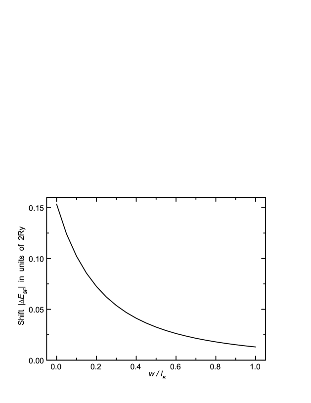
Figure 1: The CSFE exchange shift is calculated from the formula of Eq. (21) with the modified Coulomb interaction $V(q)\!=\!q^{-1}e^{q^{2}w^{2}}\mbox{erfc}(qw)$; the shift value absolute at $w\!=\!0$ is $(1-\ln{2})/2$.

References

• (1) W. Kohn, Phys. Rev., $123$, 1242 (1961).
• (2) C. Kallin and B. I. Halperin, Phys. Rev. B 30, 5655 (1984).
• (3) A. Pinczuk et al., Phys. Rev. Lett. 68, 3623 (1992).
• (4) L.V. Kulik, I.V. Kukushkin, S. Dickmann, V.E. Kirpichev, A.B. Van’kov, A.L. Parakhonsky, J.H. Smet, K. v. Klitzing, and W. Wegscheider, to appear (cond-mat/0501466).
• (5) S. Dickmann, Phys. Rev. B 65, 195310 (2002).
• (6) A.B. Dzyubenko and Yu.E. Lozovik, Sov. Phys. Solid State 25, 874 (1983) [ibid. 26, 938 (1984)].
• (7) S. Dikman, and S. V. Iordanskii, JETP 83, 128 (1996); S. Dickmann and Y. Levinson, Phys. Rev. B 60 7760 (1999); S. Dickmann, Phys. Rev. B 61, 5461 (2000); and Phys. Rev. Lett. 93, 206804 (2004).
• (8) Yu.A. Bychkov, and S.V. Iordanskii, Sov. Phys. Solid State 29, 1405 (1987).
• (9) Yu.A. Bychkov, and E.I. Rashba, JETP 58, 1062 (1983).
• (10) L.D. Landau and E.M. Lifschitz, Quantum Mechanics (Butterworth-Heinemann, Oxford, 1991).
• (11) E.g. these terms are available in the second order corections to the skyrmion-antiskyrmion gap [6] and to the energy of the hole at the ${\mbox{\footnotesize${\cal V}$}}\!=\!1$ filling. We remark that the hole energy correction was calculated in Ref. [6] without taking into account the twofold-integration contribution. The latter constitutes $-0.00349$ (in the strict 2D limit) and has to be added to the result $-\pi^{2}/24\!+\!\frac{3}{4}(\ln{2})^{2}$ presented there. The total correction is thereby $-0.0544$ in units of 2Ry (cf. the numerical result in Ref. [14]).
• (12) N.R. Cooper, Phys. Rev. B 55, 1934 (1997).
• (13) M.A. Eriksson et al., Phys. Rev. Lett. 82, 2163 (1999).
• (14) S.L. Sondhi et al., Phys. Rev. B 47, 16419 (1993).
Refer to caption