Statistics of Polymer Extension in a Random Flow with Mean Shear

Abstract

Considering the dynamics of a polymer with finite extensibility placed in a chaotic flow with large mean shear, we explain how the statistics of polymer extension changes with Weissenberg number, ${\it Wi}$, defined as the product of the polymer relaxation time and the Lyapunov exponent of the flow. Four regimes, of the ${\it Wi}$ number, are identified. One below the coil-stretched transition and three above the coil-stretched transition. Specific emphasis is given to explaining these regimes in terms of the polymer dynamics.

Introduction. Recently a number of experimental observations resolving the dynamics of individual polymers (DNA molecules) in a permanent shear flow have been reported by [Smith et al. (1999)], see also [Hur et al. (2001)]. These experimental results and the subsequent theoretical/numerical study of [Hur et al. (2000)] have focused on the analysis of the power spectral density and simultaneous PDF of the polymer extension in the permanent shear, with fluctuations driven by thermal noise. In another experimental development by Groisman & Steinberg (2000,2001,2004), a chaotic flow state called by the authors “elastic turbulence” was observed in dilute polymer solutions. This flow consists of regular (shear-like) and chaotic components, the latter being weaker. Resolving an individual polymer in this chaotic steady flow was the next challenging but still accessible task achieved by [Gerashchenko et al. (2004)]. The coil-stretch transition, predicted by [Lumley (1973)] (see also [Balkovsky et al. (2000)] and [Chertkov (2000)]), was observed in direct single-polymer measurements by [Gerashchenko et al. (2004)].

In this letter we present a theoretical analysis of the polymer extension statistics in a chaotic flow with large mean shear, $s$, e.g. of the type corresponding to the elastic turbulence setup described by Groisman & Steinberg (2000,2001,2004). It is assumed that the flow is statistically steady and thus the polymer attains a statistically steady distribution as well. We establish the main features of the extension probability distribution, paying special attention to the PDF tails.

The structure of this letter is as follows. We begin introducing the basic dumb-bell-like equation governing dynamics of the polymer end-to-end vector, $\bm{R}$, in a non-homogeneous flow. Even though the prime interest of this letter is to describe the statistics of the polymer extension, $R$ (the absolute value of $\bm{R}$) the dynamics of $R$ is tightly linked to the angular dynamics. This angular dynamics and the related statistics were the subjects of our recent study, see [Chertkov et al. (2004)]. A brief explanation of these recent results, relevant to this letter concludes our introduction. We then focus on the main subject - to describe the statistics of the polymer extension. We formulate the basic stochastic equation governing the dynamics of the polymer extension. Then we analyze the structure of the extension PDF which shows a strong dependence on the Weissenberg number, ${\it Wi}$. We consider four cases corresponding to qualitatively different PDF behaviors. We explain how the typical extension depends on ${\it Wi}$ and examine the tails of the extension PDF, for $R$ less than and larger than typical values. The structure of the tails is complicated, consisting in some cases of a number of asymptotic sub-intervals. We explain the dynamical origin of all the sub-intervals. To illustrate our generic analytical results, we present in Fig. 2 graphs, corresponding to the four different regimes, obtained by direct numerical simulation made within a model of short-correlated velocity statistics and of the so-called FENE-P modeling of polymer elasticity.

Model. We consider a single polymer molecule which is advected by a chaotic/turbulent flow (i.e. the polymer moves along a Lagrangian trajectory of the flow) and is stretched by velocity inhomogeneity. The polymer stretching is characterized by the molecule’s end-to-end separation vector, ${\bm{R}}$, satisfying the following dumb-bell-like equation (see e.g. [Hinch (1977), Bird et al. (1987)]):

$$\partial_{t}R_{i}=R_{j}\nabla_{j}v_{i}-\gamma(R)R_{i}+\zeta_{i}\,.$$ (1)

Here $\gamma$ is the polymer relaxation rate and $\zeta_{i}$ is the Langevin force. The velocity gradient $\nabla_{j}v_{i}$ is taken at the molecule position. The velocity difference between the polymer end points is approximated in Eq. (1) by the first term of its Taylor expansion in the end-to-end vector. This approximation is justified if the polymer size is less than the velocity correlation length. The relaxation rate $\gamma$ in Eq. (1) is a function of the extension $R$ which varies from zero upto a maximum value $R_{\mathrm{max}}$ corresponding to a fully stretched polymer. We assume that the relaxation is Hookean for $R\ll R_{\mathrm{max}}$, i.e. $\gamma(R)$ is well approximated by a constant $\gamma_{0}$ there, while it diverges (the polymer becomes stiff) for $R\to R_{\mathrm{max}}$.

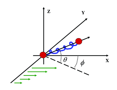
Figure 1: Scheme explaining polymer orientation geometry.

We focus on the situation in which the effect of velocity fluctuations is stronger than that of thermal fluctuations, so that the Langevin force $\bm{\zeta}$ in Eq. (1) can be neglected. We consider the case in which the steady shear flow is accompanied by weaker random velocity fluctuations. This is also the setting realized in the elastic turbulence experiments by Groisman & Steinberg (2000,2001,2004). We choose the coordinate frame associated with the shear flow, as shown in Fig. 1, where the mean shear flow is characterized by the velocity $(sy,0,0)$ and $s$ is positive. Then the polymer end-to-end vector $\bm{R}$ is conveniently parameterized by the spherical angles $\phi$ and $\theta$: $R_{x}=R\cos\theta\cos\phi$, $R_{y}=R\cos\theta\sin\phi$, $R_{z}=R\sin\theta$. In terms of these variables, Eq. (1) (with the Langevin term omitted) transforms into the following set of equations:

$$\partial_{t}{\phi}=-s\sin^{2}\phi+\xi_{\phi}\,,$$ (2)

$$\partial_{t}{\theta}=-s\sin\phi\cos\phi\sin\theta\cos\theta+\xi_{\theta}\,,$$ (3)

$$\partial_{t}\ln R=-\gamma(R)+s\cos^{2}\theta\cos\phi\sin\phi+\xi_{\parallel}\,,$$ (4)

where $\xi_{\phi}$, $\xi_{\theta}$ and $\xi_{\parallel}$ are random variables related to the fluctuating component of the velocity gradient. Note, that the angular (orientational) dynamics described by Eqs. (2,3) decouples from the dynamics of the polymer extension, $R$. Another remark is that, at $\gamma=0$, Eq. (4) describes the divergence of neighboring Lagrangian trajectories.

The character of the angular dynamics (closely related to the Lagrangian dynamics in the flow) was discussed in detail by [Chertkov et al. (2004)]. Typically, the polymer orientation fluctuates near its preferred direction determined by the shear. Characteristic values of the fluctuations, both in $\theta$ and $\phi$, are determined by the average value of the angle $\phi$, $\phi_{t}$, while the average value of $\theta$ is zero. (We consider parametrization with the angles taken inside the torus $-\pi/2<\phi,\theta<\pi/2$.) The value of $\phi_{t}$ is small due to assumed weakness of the velocity gradient fluctuations $\xi$ in comparison with the shear rate $s$. Note that $\phi_{t}$ is directly related to the value of the Lyapunov exponent of the flow, $\bar{\lambda}$: $\bar{\lambda}=s\phi_{t}$. We make the natural assumption that the flow velocity is correlated at the time $\tau_{t}=\bar{\lambda}^{-1}$. The random terms $\xi_{\phi}$ and $\xi_{\theta}$ in Eqs. (2,3) are relevant (i.e. comparable to their deterministic counter-parts) only in the narrow angular region $|\phi|,|\theta|<\phi_{t}$. Outside this “stochastic domain” the angular dynamics is mainly deterministic, i.e. the effect of the stochastic terms, $\xi_{\phi}$ and $\xi_{\theta}$, is not essential there. The deterministic motion leads to polymer flipping (i.e. reversing its orientation). The flips interrupt slower stochastic wandering near the shear-preferred direction. The process of the deterministic/stochastic regimes alteration (tumbling) is a-periodic.

The Statistics of Polymer Extension. We consider the case of a statistically steady random flow, that leads to stationary statistics as a function of the angles, $\theta,\phi$, and of the extension $R$. Our goal here is to describe the statistics of $R$ that emerges as a result of the balance between elasticity-driven contraction and extension, caused by fluctuations in the flow.

For the principal part of the dynamics, the basic dynamical equation Eq. (4) can be simplified. First, the main contribution to the $R$ dynamics stems from the region of small angles where $\sin\phi$ can be replaced by $\phi$ and $\cos\theta$ by unity. Second, the term $\xi_{\parallel}$ is potentially important only in the stochastic region where $\xi_{\phi}$ competes with $s\phi^{2}$. However, assuming $\xi_{\phi}\sim\xi_{\parallel}$, we conclude that $\xi_{\parallel}$ is negligible in comparison with $s\phi$ there. Therefore one arrives at:

$$\partial_{t}\ln R=-\gamma(R)+s\phi\,.$$ (5)

Note that Eq. (5) is inapplicable when $R$ is close to its minimum value during a flip (since the angles $\phi,\theta$ are of order unity there). Another remark is that Eq. (5) is correct for $R\gg R_{T}$ ($R_{T}$ is the typical length of the polymer in the absence of the flow) where the Langevin force can be neglected.

The statistics of $R$ is determined by the interplay of the two terms on the right-hand side of Eq. (5). Since the average value of $s\phi$ is equal to the Lyapunov exponent, $\bar{\lambda}$, the dimensionless parameter characterizing the statistics of the polymer extension is the Weissenberg number, ${\it Wi}\equiv\bar{\lambda}/\gamma_{0}$, which grows with the strength of the shear, or/and, of the velocity fluctuations. At ${\it Wi}=1$, when the two terms on the right hand side of Eq. (5) balance each other, the system undergoes the so-called coil-stretched transition, see [Lumley (1969), Lumley (1973), Balkovsky et al. (2000), Chertkov (2000)] and [Balkovsky et al. (2001)] for details. We find, however, that in the specific case of strong shear considered in the letter additional qualitative changes in the PDF of $R$ occur at ${\it Wi}>1$ so that the overall picture is richer than the case of isotropic velocity statistics. Below we describe characteristic features of the extension PDF as a function of ${\it Wi}$.

To illustrate our generic analytical results we plot in Fig. 2 four graphs of the extension PDF obtained by numerical simulations based on modification of Eq. (5), $\partial_{t}\ln R=-\gamma+s\sin\phi\cos\phi$, which allows the correct reproduction of the flips, and Eq. (2) with the stochastic term $\xi_{\phi}$ chosen to be $\delta$-correlated in time. The simulations were done with $\gamma(R)=\gamma_{0}/(1-R^{2}/R^{2}_{\mathrm{max}})$, corresponding to the so-called FENE-P model of the polymer elasticity, see e.g. [Bird et al. (1987)].

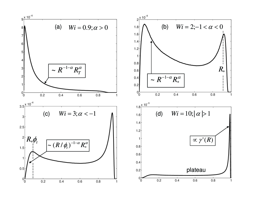
Figure 2: PDF of the polymer extension, $R$, measured in the units of maximal extension, for different values of the Weissenberg number, ${\it Wi}$, obtained from numerical simulations of the stochastic equations explained in the text.

${\it Wi}<1$, $\alpha>0$. We begin by discussing the case ${\it Wi}<1$, for which the polymer is only weakly stretched. Then, typically, the molecule stays in the “coil” state characterized by the thermal size, $R_{T}$, which emerges as the result of a balance between the Langevin driven extension and contraction (relaxation) related to polymer elasticity. Let us recall that due to a large number of monomers in the polymer molecule, the thermal noise induced length, $R_{T}$, is much smaller than the maximal polymer extension, $R_{\mathrm{max}}$.

At the scales larger than $R_{T}$ the thermal noise is irrelevant and the extension dynamics is described by Eq. (5). Being interested in the statistics for large, $R\gg R_{T}$, for deviations from the typical value, $R_{T}$, one comes to a problem that was already analyzed in detail by [Balkovsky et al. (2000), Chertkov (2000), Balkovsky et al. (2001)], in which it was shown that the extension PDF has an algebraic tail:

$$P(R)\propto R^{-1-\alpha}\,,$$ (6)

with $\alpha>0$. Eq. (6) holds at $R_{\mathrm{max}}\gg R\gg R_{T}$ where $\gamma(R)$ weakly deviates from $\gamma_{0}$. The situation is reflected in Fig. 2a, where the algebraic tail is clearly seen. The positive value of the exponent $\alpha$ in Eq. (6) guarantees that the normalization integral $\int dR\,P(R)$ converges in the region $R\gg R_{T}$. Thus, the normalization coefficient in Eq. (6) is $\sim R_{T}^{-\alpha}$. The exponent $\alpha$ decreases as the Weissenberg number, ${\it Wi}$, increases, and it crosses zero at the coil-stretch transition, where ${\it Wi}=1$.

The algebraic tail (6) is related to a long (compared to the correlation time $\tau_{t}$) process of polymer extension from the typical value $R_{T}$ to the current value of the extension, $R\gg R_{T}$. Note that this long extension does not mean that (during the process of extension) the right hand side of Eq. (5) is always positive since $\phi$ fluctuates and $s\phi$ is larger than $\gamma$ only on average. Moreover, the process consists of alternating stochastic and deterministic portions (polymer flips during the later ones). In spite of the fact that $R$ decreases during the first half of the flip, the initial extension is restored (returns to its initial value) during the second half of the flip. Overall, the flips do not influence the extension process. The probability $W$ of this a-typically long extension process depends exponentially on its duration $T$, since $W$ is a product of independent probabilities, each representing a sub-processes of duration $\tau_{t}$. This gives the following estimate: $\ln W\sim-T/\tau_{t}$. On the other hand, in accordance with Eq. (5), $\ln(R/R_{T})\sim T/\tau_{t}$. Combining the two estimates, we arrive at the algebraic tail (6) for the PDF of extension, $P=dW/dR$.

${\it Wi}>1$, $-1<\alpha<0$. Above the coil-stretch transition, when $\bar{\lambda}$ exceeds $\gamma_{0}$, the polymers become strongly extended. In this stretched state the typical size of the polymer, $R_{*}$, is much larger than $R_{T}$. Considering the stationary average of Eq. (5) one finds that $\gamma(R_{*})=\bar{\lambda}$.

The left tail of the PDF, corresponding to $R_{T}\ll R\ll R_{*}$, is governed by the same algebraic law (6). However, now $\alpha<0$, meaning that the normalization integral $\int dR\,P(R)$ gets a major contribution for $R\sim R_{*}$. Therefore, restoring normalization, one derives $P\sim R_{*}^{\alpha}R^{-1-\alpha}$ for the $R\ll R_{*}$ tail. The transition from positive to negative $\alpha$ corresponds to important change in the nature of the dynamical configuration corresponding to the algebraic tail: extension, as a typical process for $\alpha>0$, is replaced by contraction for negative $\alpha$, so that initially typical extension, $\sim R_{*}$, contracts through a long, $T\gg\tau_{t}$, (multi-tumbling) evolution. (Physical arguments, clarifying the origin of the algebraic tail, are identical to the ones presented above for ${\it Wi}<1$.)

The right tail, corresponding to extreme extensions, $R_{\mathrm{max}}-R\ll R-R_{*}$, can also be explained in some general terms. The domain of extreme deviation is characterized by extremely fast relaxation, so that the term on the left hand side of Eq. (5) can be neglected. As a result, $R$ and $\phi$ are related to each other locally: $\gamma(R)=s\phi$. Moreover, one finds that, because of the fast nature of the polymer relaxation in the extreme case, $\phi$ simply follows the respective random term in Eq. (2), i.e. the term on the left hand side of Eq. (2) can also be neglected resulting in, $s\phi^{2}=\xi_{\phi}$. In other words, the extreme configuration is produced through fast anti-clockwise revolution of the polymer to a large (in comparison with the typical value $\phi_{t}$) positive angle, $1\gg\phi\gg\phi_{t}$, driven by anomalous fluctuations in $\xi_{\phi}$. Recalculating the PDF of $\xi_{\phi}$ into $P(R)$ one arrives at

$$P(R)=2s^{-1}\gamma\gamma^{\prime}P_{\xi}(\gamma^{2}/s)\,,$$ (7)

where $P_{\xi}$ is the simultaneous PDF of the velocity gradient term $\xi_{\phi}$. Note that the asymptotic expression given by Eq. (7) is not restricted to the case considered in this subsection but applies generically to the description of extreme polymer extensions in all regimes.

${\it Wi}>1$, $\alpha<-1$. Once $\alpha$ crosses $-1$, $R_{*}$ becomes maximum of the extension PDF, $P(R)$. This modification in the PDF shape is accompanied by the emergence of a plateau on the left from the maximum (see Fig. 2c), associated with an additional contribution to the PDF related to the deterministic angular dynamics.

Let us explain the origin of the plateau. For angles which are smaller than unity but larger than $\phi_{t}$, $R$ and $\phi$ satisfy, $\partial_{t}\ln R=s\phi$ and $\partial_{t}\phi=-s\phi^{2}$, as follows from Eqs. (2,5). Integrating these equations one arrives at, $R=A|t-t_{0}|$ where $t_{0}$ and $A$ are constants, the latter being estimated by $A\sim R_{*}/\tau_{t}$. Taking into account the fact that the time $t_{0}$ is homogeneously distributed (due to the assumed homogeneity of the velocity statistics), and recalculating the measure $dt_{0}$ into the PDF of $R$, one arrives at $P(R)=C/R_{*}$ ($C$ is an $R$-independent constant of order unity) corresponding to the plateau seen in Fig. 2c.

The “deterministic” contribution to $P(R)$, $\sim 1/R_{*}$, discussed above, does not cancel the “stochastic” one $\sim R_{*}^{\alpha}R^{-1-\alpha}$ corresponding to the long contraction which starts at $R_{*}$. In fact these contributions co-exist. One finds that for $-1<\alpha<0$, the stochastic contribution dominates, in full agreement with the above discussion of Fig. 2b. When $\alpha$ becomes smaller than $-1$, the situation is reversed and the deterministic contribution dominates.

The plateau extends from $R\sim R_{*}$ down to $R\sim R_{*}\phi_{t}$, where $R_{*}\phi_{t}$ is the smallest value of $R$ one can achieve under the condition that when the flip begins the initial extension is $R_{*}$. Note however, that if the initial extension is smaller than $R_{*}$, a deterministic flip could bring it to values that are smaller than $R_{*}\phi_{t}$. Therefore, to understand even smaller values of $R$, $R<R_{*}\phi_{t}$, one should consider flips which begin with an anomalously small initial value $R_{0}$, $R_{0}<R_{*}$ (prepared by some preliminary and long stochastic processes, of the type discussed above). The probability density of achieving $R_{0}$ during the preparatory stage is estimated according to Eq. (6): $\sim R_{*}^{\alpha}R_{0}^{-1-\alpha}$. On the other hand, any $R_{0}$ that lies between $R$ and $R/\phi_{t}$ transforms dynamically as a result of a fast flip into the current value of extension $R$ with the same $R$-independent probability, which now can be estimated as $\sim 1/R_{0}$. Therefore, one arrives at the following estimate for the PDF of $R$ at $R<R_{*}\phi_{t}$:

$$P\sim\int_{R}^{R/\phi_{t}}\frac{dR_{0}}{R_{0}}\times\frac{R_{*}^{\alpha}}{R_{0}^{1+\alpha}}\sim R_{*}^{-|\alpha|}\left(\frac{R}{\phi_{t}}\right)^{|\alpha|-1}.$$ (8)

Eq. (8) explains the probability decrease at the smallest $R$ seen in Fig. 2c.

Let us observe the bump in Fig. 2c separating the region of the plateau and the smallest $R$ region of the probability decay. To explain the bump, one simply needs to account for the angular nonlinearity (with respect to $\phi$ and $\theta$) in the estimate of the plateau just discussed.

${\it Wi}\gg 1$, $\alpha\ll-1$. The larger ${\it Wi}$ is, the closer $R_{*}$ approaches $R_{\mathrm{max}}$. Then the condition of fast relaxation, $R\gamma^{\prime}(R)\gg\gamma$, which has already allowed us to analyze the extreme asymptotics (7), also applies to the region in the vicinity of $R_{*}$. The smallness of the ratio $\gamma/(R\gamma^{\prime})$ suggests that the left hand side of Eq. (5) can be replaced by zero. One arrives at $\gamma(R)=s\phi$, which makes it easy to express the PDF of $R$ through the simultaneous PDF of $\phi$:

$$P(R)\sim s^{-1}\gamma^{\prime}(R)P_{\phi}(\gamma/s)\,,$$ (9)

where it is also assumed that $\gamma(R)/s<\phi_{t}$. In this special domain of $R$ and $\phi$, variations of $P_{\phi}$ are slow, so that the main dependence on $R$ in Eq. (9) is due to the factor $\gamma^{\prime}(R)$. Eq. (9) applies to the left (for smaller values of $R$) of $R_{*}$ provided the parameter $R\gamma^{\prime}(R)/\gamma$ is large. In this domain, the PDF can be estimated as $P\sim\gamma^{\prime}(R)/\gamma(R_{*})$. At even smaller values of $R$, the PDF has a plateau, $P\sim\gamma_{0}/[R_{*}\gamma(R_{*})]$ (which generalizes our previous result to the ${\it Wi}\gg 1$ case). This explains the complex behavior of the PDF of $R$ shown in Fig. 2d.

Conclusions. In this second work devoted to the statistics of polymer molecules in a chaotic flow with mean shear, we focused on analyzing the statistics of the polymer extension $R$. The PDF of $R$ demonstrates complex and rich ${\it Wi}$-dependent behavior related to a number of distinct processes governing polymer dynamics. We observed that the typical value of the extension associated with the stochastic wandering of the polymer orientation around the special shear-preferred direction increases with ${\it Wi}$. In the region of maximal stretching, near $R_{\mathrm{max}}$, the major contribution to the PDF originates from processes characterized by fast adjustment of the polymer extension to the current value of the polymer’s angular degree of freedom. We also identified special contributions to the PDF tails associated with fast (deterministic) flips and long (stochastic) extension or contraction processes. Encouraged by qualitative agreement of our results with the newest experimental data of [Gerashchenko et al. (2004)], we anticipate that the rich zoo of theoretical predictions presented in the paper will be helpful for guiding and testing future experimental work in this field.

We thank A. Celani and V. Steinberg for stimulating discussions and G. D. Doolen for useful comments. Support of RSSF through personal grant (IK), RFBR grant 04-02-16520a (IK,VL and KT), and a grant from the Dynasty Foundation (KT) are acknowledged.

References

- [Balkovsky et al. (2000)] Balkovsky, E., Fouxon, A., & Lebedev, V. 2000 Turbulent dynamics of polymer solutions Phys. Rev. Lett. 84, 4765–4768. (2000)
- [Balkovsky et al. (2001)] Balkovsky, E., Fouxon, A., & Lebedev, V. 2001 Turbulence of polymer solutions Phys. Rev. E 64, 056301.
- [Bird et al. (1987)] Bird, R.B., Curtiss, C.F., Armstrong, R.C., & Hassager 1987 Dynamics of Polymeric Liquids Wiley, New York.
- [Chertkov (2000)] Chertkov, M. 2000 Polymer Stretching by Turbulence Phys. Rev. Lett. 84, 4761–4764.
- [Chertkov et al. (2004)] Chertkov, M., Kolokolov, I., Lebedev, V., & Turitsyn, K. 2004 Tumbling of Polymers in Random Flow with Mean Shear Los Alamos Preprint LA-UR-04-1871.
- [Gerashchenko et al. (2004)] Gerashchenko, S, Chevallard, C., & Steinberg, V. 2004 Single polymer dynamics: coil-stretch transition in a random flow Submitted to Nature.
- [Groisman & Steinberg (2000)] Groisman, A., & Steinberg, V. 2000 Elastic turbulence in a polymer solution flow Nature 405, 53–55.
- [Groisman & Steinberg (2001)] Groisman, A., & Steinberg, V. 2001 Stretching of polymers in a random three-dimensional flow Phys.Rev.Lett. 86, 934–937.
- [Groisman & Steinberg (2004)] Groisman, A., & Steinberg, V. 2004 Elastic turbulence in curvilinear flows of polymer solutions New. J. Phys. 6, 29.
- [Hinch (1977)] Hinch, E.J. 1977 Mechanical models of dilute polymer solutions in strong flows Phys. Fluids 20, S22–S30.
- [Hinch & Leal (1972)] Hinch, E.J., & Leal, L.G. 1972 The effect of Brownian motion on the rheological properties of a suspension of non-spherical particles J. Fluid Mech. 52, 683–712.
- [Hur et al. (2000)] Hur, J. S., Shaqfeh, E.S.G., Larson, R. G. 2000 Brownian dynamics of single DNA molecules in shear flow, J. Rheol. 44, 713–742.
- [Hur et al. (2001)] Hur, J. S., Shaqfeh, E.S.G., Babcock, H. P., Smith, D. E., Chu, S. 2001 Dynamics of dilute and semidilute DNA solutions in the start-up of shear flow, J. Rheol. 45, 421–450.
- [Lumley (1969)] Lumley, J.L. 1969 Drag reduction by additives Ann. Rev. Fluid Mech. 1, 367.
- [Lumley (1973)] Lumley, J.L. 1973 Drag reduction in turbulent flow by polymer additives J. Polymer Sci.: Macromolecular Reviews 7, 263–290.
- [Smith et al. (1999)] Smith, D. E., Babcock, H.P., Chu, S. 1999 Single-polymer dynamics in steady shear flow Science 283, 1724–1727.