Tumbling of Polymers in a Random Flow with Mean Shear

Abstract

A polymer placed in chaotic flow with large mean shear tumbles, making a-periodic flips. We describe the statistics of angular orientation, as well as of tumbling time (separating two subsequent flips) of polymers in this flow. The probability distribution function (PDF) of the polymer orientation is peaked around a shear-preferred direction. The tails of this angular PDF are algebraic. The PDF of the tumbling time, $\tau$, has a maximum at the value estimated as inverse Lyapunov exponent of the flow. This PDF shows an exponential tail for large $\tau$ and a small-$\tau$ tail determined by the simultaneous statistics of velocity PDF.

Introduction. With the development of novel optical methods a number of high quality experimental observations resolving individual polymer (e.g. DNA molecule) dynamics for elongational and shear regular flows have been reported by [Perkins et al. (1997)], [Smith & Chu (1998)] and by [Smith et al. (1999)] and [Hur et al. (2001)], respectively. Experimental explorations by [Smith et al. (1999)] and the subsequent theoretical/numerical study by [Hur et al. (2000)] of the shear flow setting had focused on the analysis of the power spectral density and the simultaneous statistics of polymer extension, for the case in which fluctuations are driven by thermal noise. Additionally, one noticeable phenomenon, called tumbling, was reported by [Smith et al. (1999)] for the regime of strong shear flow: The molecule which spends most of the time being oriented along the direction dictated by the shear sometimes and suddenly (a-periodically) flips. In another experimental breakthrough, a chaotic flow state called by the authors “elastic turbulence” was observed for dilute polymer solutions by Groisman & Steinberg (2000,2001,2004). This flow consists of regular (shear-like) and chaotic components, the latter being weaker. Resolving an individual polymer in this steady chaotic flow was more challenging than in the regular flow experiment but still it appeared to be an accessible task for [Gerashchenko et al. (2004)]. The coil-stretch transition, predicted by Lumley (1969,1973) (see also Balkovsky et al. (2000,2001) and [Chertkov (2000)]), was observed, for the first time, in direct single-polymer measurements by [Gerashchenko et al. (2004)]. The statistics of the polymer extension and of the tumbling time were also tested in the elastic turbulence experiments, however the phenomenon has not yet been fully explored.

In this letter, we discuss the statistics of polymers placed in a chaotic flow with a relatively large mean shear, that is the flow of the type correspondent to the elastic turbulence experiments by Groisman & Steinberg (2000,2001,2004). We assume that the effect of velocity fluctuations is stronger than that related to thermal noise and that polymers are essentially elongated due to the fluctuations so that the polymer orientation is well defined. The main body of the orientational fluctuations occur in a neighborhood of a special direction preferred by the shear. Sometimes these typical fluctuations around the preferred direction are interrupted by flips, in which the polymer orientation is reversed. The task of this study is to describe the statistics of the angular orientation and tumbling time.

The structure of this letter is as follows. We begin by introducing the basic dumb-bell-like equation governing the dynamics of the polymer end-to-end vector in a non-homogeneous flow. If the effect of thermal fluctuations is negligible, the angular part of the polymer dynamics decouples from its extensional counterpart and can be examined separately. It is convenient to count the angular degrees of freedom $\phi$ and $\theta$ (for in-plane and off-plane orientations, respectively) from the direction prescribed by the shear. We show that the angular PDF is peaked at some small angle $\phi$, estimated by the average value $\phi_{t}=\langle\phi\rangle$, $\phi_{t}\ll 1$. The widths (in both angles) of the main part of the PDF are of the order of $\phi_{t}$. Then we demonstrate that tails of the joint PDF are algebraic at $\phi_{t}\ll\phi,\theta\ll 1$. We find that this algebraic tail of the individual PDF of $\phi$ is related to purely deterministic (i.e. shear driven) dynamics: ${\cal P}(\phi)\propto\sin^{-2}\phi$. The tail of the $\theta$ PDF has two competing contributions, one related to deterministic dynamics, $\propto\theta^{-2}$ for $\phi\ll|\theta|\ll 1$, and the other one related to stochastic dynamics, $\propto\theta^{-a}$, where $a$ is a number, dependent on details of the velocity fluctuation statistics. Then we examine the statistics of the tumbling time, $\tau$, that is defined as the time between two subsequent flips of the polymer. The PDF of $\tau$ is peaked at a time estimated by the inverse Lyapunov exponent of the flow, $\tau_{t}=\bar{\lambda}^{-1}$. The long time, $\tau\gg\tau_{t}$, tail of the PDF is exponential, $\ln[P(\tau)]\sim-\tau/\tau_{t}$. The statistics of small tumbling times is related to the simultaneous PDF of the velocity gradients. To derive these results we explore the close relation between the stochastic dynamics of $\theta$ and $\phi$ and Lagrangian dynamics of the flow.separation in the flow. We conclude by discussing the applicability conditions for our approach and the validity of the assumptions made in this letter.

Model. We consider a single polymer molecule which is advected by a chaotic/turbulent flow. We assume that the velocity correlation length is much larger than the size of the polymer. (Note, that this condition is always satisfied in elastic turbulence simply because the velocity correlation length coincides with the overall size of the flow/apparatus that is the biggest scale in the problem.) Then the polymer can be viewed as a material point moving along a Lagrangian trajectory. In addition, the polymer is stretched due to the flow inhomogeneity. The polymer stretching can be characterized by its end-to-end separation vector, ${\bm{R}}$. The stochastic dynamics of the vector ${\bm{R}}$ can be examined in the framework of the following dumb-bell-like equation (see e.g. [Hinch (1977)] and [Bird et al. (1987)])

$$\partial_{t}R_{i}=R_{j}\nabla_{j}v_{i}-\gamma R_{i}+\zeta_{i}\,,$$ (1)

where $\gamma$ is the polymer relaxation rate (dependent on $R$, the absolute value of the vector $\bm{R}$), the velocity gradient $\nabla_{j}v_{i}$ is taken at the molecule position, and $\zeta_{i}$ is the Langevin force. The velocity difference between the end points of the polymer is approximated in Eq. (1) by the first term of its Taylor expansion in the end-to-end vector. This is justified by the smallness of the polymer extension $R$ in comparison with the velocity correlation length.

We focus on the situation for which the effect of velocity fluctuations is stronger than the effect of thermal noise. Then the Langevin force in Eq. (1) can be neglected. In this case the polymer angular (orientational) dynamics described by the unit vector $\bm{n}=\bm{R}/R$ decouples from the dynamics of the end-to-end polymer length $R$ and one derives from Eq. (1) a closed equation for $\bm{n}$:

$$\partial_{t}n_{i}=n_{j}(\delta_{il}-n_{i}n_{l})\nabla_{j}v_{l}\,.$$ (2)

Note that Eq. (2) coincides with the dynamics of a rod-like micro-object immersed in the same flow.

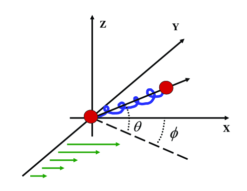
Figure 1: Schematic figure explaining polymer orientation geometry.

Let us choose the coordinate frame associated with the mean shear velocity, as shown in Fig. 1. In this reference frame the mean flow is characterized by the velocity $(sy,0,0)$ where $s$ is assumed to be positive. The polymer orientation is conveniently parameterized in terms of the angles $\phi$ and $\theta$: $n_{x}=\cos\theta\cos\phi$, $n_{y}=\cos\theta\sin\phi$, $n_{z}=\sin\theta$. Then, Eq. (2) becomes

$$\partial_{t}{\phi}=-s\sin^{2}\phi+\xi_{\phi}\,,$$ (3)

$$\partial_{t}{\theta}=-s\sin\phi\cos\phi\sin\theta\cos\theta+\xi_{\theta}\,,$$ (4)

where $\xi_{\phi}$ and $\xi_{\theta}$ are random variables related to the fluctuation component of the velocity gradient.

Angular statistics. The statistics of the velocity fluctuations is assumed to be homogeneous in time. In a statistically stationary velocity field, the angular statistics is stationary as well, being characterized by the joint PDF, ${\cal P}(\phi,\theta)$, which is a periodic function of the angles with the period $\pi$ for both $\phi$ and $\theta$. Thus, it is sufficient to consider ${\cal P}(\phi,\theta)$ within the following bounded domain (torus), $-\pi/2<\phi,\theta<\pi/2$. We normalize the PDF using $\int d\phi\,d\theta\,{\cal P}(\phi,\theta)=1$, where the integral is taken over the domain. Note, that according to the structure of Eqs. (3,4), $\cal P(\phi,\theta)$ is symmetric with respect to $\theta$ but it is not symmetric with respect to $\phi$. Therefore, the average value of $\phi$, $\phi_{t}=\langle\phi\rangle$, is non-zero. In our setting, $\phi_{t}$ is positive. The value of $\phi_{t}$ can be estimated by balancing the deterministic and stochastic terms on the right hand side of Eq. (3). The weakness of the random term in comparison with $s$ implies $\phi_{t}\ll 1$. The same quantity $\phi_{t}$ estimates typical fluctuations of $\phi$ about its mean value. Once one assumes that the random terms in Eqs. (3,4) are comparable, it immediately follows that typical value of $\theta$ fluctuations is estimated by $\phi_{t}$ as well.

Note that the equation, $\partial_{t}r_{i}=r_{j}\nabla_{j}v_{i}$, describing dynamics of separation between two neighboring fluid particles (moving along nearby Langangian trajectories), leads to the same dynamics for the unit vector $\bm{r}/r$ as determined by Eq. (2) and, consequently, to the same angular dynamics as described by Eqs. (3,4). For $r$ (the absolute value of ${\bm{r}}$) one derives: $\partial_{t}\ln r=s\cos^{2}\theta\cos\phi\sin\phi+\xi_{\parallel}$, where $\xi_{\parallel}$ represents the direct (as opposed to indirect through fluctuations in $\phi$) effect of velocity fluctuations. It follows from Eq. (3) that for typical fluctuations (when $\phi,\theta\ll 1$) $\xi_{\phi}$ competes with $s\phi^{2}$. Assuming that $\xi_{\parallel}\sim\xi_{\phi}$ one finds that $\xi_{\parallel}$ is negligible in comparison with $s\phi$, because the relevant values of $\phi$ are small, $\phi\ll 1$. Therefore, for small $\phi,\theta$, one arrives at $\partial_{t}\ln r=s\phi$. This equation establishes the relation between the angular dynamics of the polymer and the dynamics of Lagrangian separation. For the Lyapunov exponent, $\bar{\lambda}$, defined as the mean logarithmic rate of divergence of Lagrangian trajectories, one finds $\bar{\lambda}=\langle\partial_{t}\ln r\rangle=s\phi_{t}$.

It is natural to expect that the Lagrangian velocity correlation time is $\tau_{t}=\bar{\lambda}^{-1}=(s\phi_{t})^{-1}$, that is also characteristic time of the $\xi_{\phi}$ and $\xi_{\theta}$ fluctuations. Then, comparing the left hand sides of Eqs. (3,4) with the first terms on their right hand sides (for $\phi,\theta\ll 1$), one concludes that the angular correlation time can be estimated by the same quantity $\tau_{t}$. Next, equating the terms on the right hand sides of Eqs. (3,4), one derives $\xi_{\phi}\sim\xi_{\theta}\sim s\phi_{t}^{2}\ll s$. The last inequality reflects the assumed weakness of the velocity gradient fluctuations compared to the shear rate, $s$.

Tails of the angular PDFs. Let us consider the domain $|\phi|,|\theta|\gg\phi_{t}$, where the random terms in Eqs. (3,4), $\xi_{\phi}$ and $\xi_{\theta}$, are negligible. The angular dynamics is purely deterministic in this domain leading to the following dependence of the angles on time $t$

$$\cot\phi=s(t-t_{0})\,,\qquad\tan\theta=c\cdot\sin\phi\,,$$ (5)

where $t_{0}$ and $c$ are some constants. According to Eq. (5), the vector $\bm{n}$ reverses its direction as $t$ increases. Therefore, Eq. (5) describes a single flip of the polymer. Due to the assumed homogeneity in time of the velocity statistics, $t_{0}$ is homogeneously distributed. Recalculating the measure $dt_{0}$ into the PDF of the angles in accordance with Eq. (5), one derives

$${{\cal P}}(\phi,\theta)=\frac{U(\tan\theta/\sin\phi)}{\sin^{3}\phi\,\cos^{2}\theta}\,.$$ (6)

The function $U$ reflects possible variations in $c$ (its statistics), which should be determined from the initial conditions for deterministic evolution. These conditions have to be found from matching Eq. (5) to those defined for the stochastic domain $|\phi|,|\theta|<\phi_{t}$. One concludes that the function $U$ is sensitive to the angular dynamics in the stochastic domain and, respectively, to details of velocity fluctuations, i.e. the function is nonuniversal. Note, that Eq. (6) is identical to the one found in [Hinch & Leal (1972)] in the context of a solid rod tumbling in shear flow caused by thermal (Langevin) fluctuations.

Eq. (5) shows that in the deterministic regime the angle $\phi$ decreases uniformly with time (that is except for the jump from $-\pi/2$ to $+\pi/2$ at $t=t_{0}$). Therefore, the stationary PDF for the angular degrees of freedom, ${\cal P}(\phi,\theta)$, corresponds to a non-zero probability flux from positive to negative $\phi$ related to a preferred (clock-wise) direction of the polymer’s rotations in the $X-Y$ plane. Formally, the probability flux goes out through $\phi=-\pi/2$ and the same flux comes back (enters) through $\phi=\pi/2$ ($\pi/2$ and $-\pi/2$ are identical by our construction) thus keeping the total probability equal to unity.

The PDF of $\phi$, $P_{\phi}$, can be obtained from the joint PDF: $P_{\phi}=\int d\theta\,{\cal P}(\phi,\theta)$. Integrating the right-hand side of Eq. (6) over $\theta$ one obtains the following expression for the tail, valid for $|\phi|\gg\phi_{t}$:

$$P_{\phi}\equiv\int d\theta\,{{\cal P}}(\phi,\theta)=C\phi_{t}\sin^{-2}\phi\,,$$ (7)

where the constant $C$ is of order unity. Let us reiterate that, thinking dynamically, Eq. (7) originates from the deterministic flips bringing $\phi$ from its most probable domain $\sim\phi_{t}$ to the observation angle. Eq. (7) describes the aforementioned probability flux: as determined by Eq. (3), $P_{\phi}\partial_{t}\phi$ is constant in the deterministic region.

Consider the PDF of $\theta$, $P_{\theta}=\int d\phi\,{\cal P}(\phi,\theta)$. The naive result for the PDF tail following from Eq. (6) is $P_{\theta}\propto|\theta|^{-2}$, provided $1\gg\theta\gg\phi$. However, one should be careful, since the expression (6) does not cover a special angular domain, characterized by $|\phi|<\phi_{t}$ and $|\theta|\gg\phi_{t}$, which should be analyzed separately. In this domain, one can neglect $\xi_{\theta}$ in Eq. (4). Assuming also $|\theta|\ll 1$, one arrives at $\partial_{t}\ln(\theta)=-s\phi$. In this case, $s\phi$ can be treated as a random variable independent of $\theta$ and the above equation leads to an algebraic tail, ${\cal P}\propto|\theta|^{-a}$, where the exponent $a$ is a positive number of order unity. The value of $a$ is sensitive to the statistics of the $\phi$ fluctuations. (Therefore, $a$ is not universal.) Let us explain the origin of the algebraic dependence. The algebraic contribution to the angular PDF is related to the long (compared to the correlation time $\tau_{t}$) period when $\phi$ fluctuates around some negative value, $\sim-\phi_{t}$. (These fluctuations can be interrupted by flips.) Then $\theta$ at the end of the $T$-long period is estimated according to $\ln(\theta/\phi_{t})\sim Ts\phi_{t}$. The probability $W$ to observe such a long a-typical period is estimated by $\ln W\sim-T/\tau_{t}$. These estimates, recalculated in the PDF of $\theta$, $P_{\theta}=dW/d\theta$, give the aforementioned algebraic tail. Note that this algebraic tail which originates from the long-time dynamics is analogous to the algebraic tail of the polymer extension PDF discussed by Balkovsky et al. (2000,2001) and [Chertkov (2000)].

Therefore, one finds that there exist two different contributions to the PDF tail: one related to the deterministic motion, described by Eq. (5), while the other is associated with the stochastic evolution in the domain, $|\phi|<\phi_{t},|\theta|\gg\phi_{t}$. For $1\gg|\theta|\gg\phi_{t}$, both contributions are algebraic, $\propto|\theta|^{-2}$ and $\propto|\theta|^{-a}$, respectively. The deterministic contribution, $\propto|\theta|^{-2}$, dominates if $a>2$, while the stochastic contribution, $\propto|\theta|^{-a}$, dominates otherwise.

Tumbling time statistics. As seen from the expression (5), the deterministic process, which actually defines the polymer turn (because $\phi$ changes essentially only during deterministic part of the dynamics), is faster than the stochastic wandering taking place at small angles, $|\phi|,|\theta|<\phi_{t}$. Therefore it is convenient to define the tumbling time, $\tau$, as the time separating two subsequent crossings in $\phi$ of the special angle $\pm\pi/2$, in the middle of the deterministic domain. Since the major contribution to $\tau$ originates from the stochastic wandering in the $\phi_{t}$-narrow vicinity of $\phi=0$, the position of the $\tau$-PDF maximum and its width are both estimated by the correlation time $\tau_{t}=(s\phi_{t})^{-1}$, because this is the only relevant characteristic time of the stochastic angular evolution.

Being interested in the PDF tail, for $\tau\gg\tau_{t}$, one observes that if a flip does not occur for a long time, then this delay can be interpreted in terms of the large number, $\tau/\tau_{t}$, of independent unsuccessful attempts to pass (clock-wise in $\phi$) the stochastic domain $|\phi|<\phi_{t}$. The probability of the delayed flip is given by the product of the probabilities of these $\tau/\tau_{t}$ events, resulting in the exponential tail of the PDF of $\tau$ for $\tau\gg\tau_{t}$, $\ln P_{\tau}\sim-\tau/\tau_{t}$.

The left, $\tau\ll\tau_{t}$, tail of the tumbling time PDF is non-universal because it is sensitive to details of the velocity field statistics. Indeed, it is determined by the special configurations of the velocity field that force $\phi$ to drift through the stochastic region a-typically fast. (Those configurations are vortices with clock-wise rotation of the fluid in the $X-Y$ plane leading to negative values of $\xi_{\phi}$ that are larger than $s\phi_{t}^{2}$ in absolute value.) Analyzing the anomalously fast revolutions of the polymer, one finds that $\xi_{\phi}$ from the right hand side of Eq. (3) may be considered as time-independent. (Here again, the natural assumption is that the correlation time of the velocity field fluctuations is of the same order as the inverse Laypunov exponent in the flow, i.e. $\sim\tau_{t}$.) Then the direct solution of Eq. (3) gives $\tau=\pi/\sqrt{|\xi_{\phi}|s}$, where we assumed that the major contribution in $\tau$ comes from the domain of small $\phi$, $\phi\ll 1$. This estimate holds if $s\gg|\xi_{\phi}|\gg s\phi_{t}^{2}$. For $1/s\ll\tau\ll\tau_{t}$ one arrives at the following expression for the PDF of $\tau$:

$$P_{\tau}=\frac{2\pi^{2}}{\tau^{3}s}P_{\xi}\left(-\frac{\pi^{2}}{\tau^{2}s}\right)\,,$$ (8)

where $P_{\xi}$ is the single-time PDF of $\xi_{\phi}$.

Conclusions. Let us discuss applicability conditions of our results. One of our assumptions was that the mean flow can be approximated by a perfect shear flow, whereas in reality flow parameters vary along the Lagrangian trajectory demonstrating essential spatial inhomogeneities. Even though these variations were not included in our derivations, our results remain valid if the variations along the Lagrangian trajectory occur on time scales larger than $\tau_{t}$ and also if the local flow does not deviate strongly from the shear configuration. Then, the PDFs discussed in this paper adjust adiabatically to the current values of the parameters and become, consequently, slow functions of spatial position. If the regular part of the flow is elongational, polymer flips become forbidden in the ideally deterministic regime while fluctuations will still generate some tumbling. Analysis of the tumbling in elongational, and, generically in any other random flow, will be discussed elsewhere.

We have focused on discussing the dynamics and the statistics of the polymer’s angular degrees of freedom. However, our theoretical scheme can be naturally extended to also include polymer extension. The stochastic dynamics and the statistical properties of the polymer extension can be examined in a way very similar to the one developed in this letter and this will be the subject of separate publication.

Our theory is based on the simple dumb-bell-like equation (1). This equation is obviously approximate, taking into account only one variable (end-to-end vector ${\bm{R}}$) of generally more complex dynamics. Therefore, it should be important to assess the effects of more realistic modeling. (This treatement should also account for internal conformational degrees of freedom.)

Note that polymer tumbling was first observed in the steady shear flow experiments of [Smith et al. (1999)] and [Hur et al. (2001)] in which orientational fluctuations were driven by thermal noise, while our analysis has focused primarily on the case of tumbling driven by velocity fluctuations. Therefore, even though all of our results are directly applicable to the elastic turbulence setting of Groisman & Steinberg (2000,2001,2004), the examination of the statistics of the Langevin driven tumbling and angular distribution is, actually, a separate task. In particular, special attention should be given to the case of extremely elongated polymers in which the non-linearity of the polymer elasticity is essential. These Langevin-related problems will be examined elsewhere. Here, let us only note the universal nature of the exponential, large $\tau$, tail of the tumbling time PDF. Indeed, it is straightforward to check that the arguments presented above are generic, thus guaranteeing that, very much like in the velocity fluctuation driven case, the tail is also exponential in the Langevin-driven case.

We thank V. Steinberg for many stimulating discussions and G. D. Doolen for useful comments. We acknowledge support of RSSF through personal grant (IK), of RFBR, grant 04-02-16520a (IK,VL and KT), and of Dynasty Foundation (KT).

References

- [Balkovsky et al. (2000)] Balkovsky, E., Fouxon, A., & Lebedev, V. 2000 Turbulent dynamics of polymer solutions Phys. Rev. Lett. 84, 4765–4768. (2000)
- [Balkovsky et al. (2001)] Balkovsky, E., Fouxon, A., & Lebedev, V. 2001 Turbulence of polymer solutions Phys. Rev. E 64, 056301.
- [Bird et al. (1987)] Bird, R.B., Curtiss, C.F., Armstrong, R.C., & Hassager 1987 Dynamics of Polymeric Liquids Wiley, New York.
- [Chertkov (2000)] Chertkov, M. 2000 Polymer Stretching by Turbulence Phys. Rev. Lett. 84, 4761–4764.
- [Gerashchenko et al. (2004)] Gerashchenko, S, Chevallard, C., & Steinberg, V. 2004 Single polymer dynamics: coil-stretch transition in a random flow Submitted to Nature.
- [Groisman & Steinberg (2000)] Groisman, A., & Steinberg, V. 2000 Elastic turbulence in a polymer solution flow Nature 405, 53–55.
- [Groisman & Steinberg (2001)] Groisman, A., & Steinberg, V. 2001 Stretching of polymers in a random three-dimensional flow Phys.Rev.Lett. 86, 934–937.
- [Groisman & Steinberg (2004)] Groisman, A., & Steinberg, V. 2004 Elastic turbulence in curvilinear flows of polymer solutions New. J. Phys. 6, 29.
- [Hinch (1977)] Hinch, E.J. 1977 Mechanical models of dilute polymer solutions in strong flows Phys. Fluids 20, S22–S30.
- [Hinch & Leal (1972)] Hinch, E.J., & Leal, L.G. 1972 The effect of Brownian motion on the rheological properties of a suspension of non-spherical particles J. Fluid Mech. 52, 683–712.
- [Hur et al. (2000)] Hur, J. S., Shaqfeh, E.S.G., Larson, R. G. 2000 Brownian dynamics of single DNA molecules in shear flow, J. Rheol. 44, 713–742.
- [Hur et al. (2001)] Hur, J. S., Shaqfeh, E.S.G., Babcock, H. P., Smith, D. E., Chu, S. 2001 Dynamics of dilute and semidilute DNA solutions in the start-up of shear flow, J. Rheol. 45, 421–450.
- [Lumley (1969)] Lumley, J.L. 1969 Drag reduction by additivies Ann. Rev. Fluid Mech. 1, 367.
- [Lumley (1973)] Lumley, J.L. 1973 Drag reduction in turbulent flow by polymer additives J. Polymer Sci.: Macromolecular Reviews 7, 263–290.
- [Perkins et al. (1997)] Perkins, T.T.,Smith, D. E., Chu, S. 1997 Single Polymer Dynamics in an Elongational Flow Science 276, 2016–2021.
- [Smith & Chu (1998)] Smith, D. E., Chu, S. 1998 Response of Flexible Polymers to a Sudden Elongational Flow Science 281, 1335–1340.
- [Smith et al. (1999)] Smith, D. E., Babcock, H.P., Chu, S. 1999 Single-polymer dynamics in steady shear flow Science 283, 1724–1727.