Collective roughening of elastic lines with hard core interaction
in a disordered environment

Abstract

We investigate by exact optimization methods the roughening of two and three-dimensional systems of elastic lines with point disorder and hard-core repulsion with open boundary conditions. In 2d we find logarithmic behavior whereas in 3d simple random walk -like behavior. The line ’forests’ become asymptotically completely entangled as the system height is increased at fixed line density due to increasing line wandering.

I Introduction

The paradigmatic model for the mixed or Shubnikov phase of a super-conductor in a magnetic field is a system of interacting elastic lines, representing the magnetic vortex lines threading the superconductor along the field direction blatter . The number of lines per unit area perpendicular to the field axis, also called the line density $\rho$, is given by the magnetic field strength and also defines the typical line-to-line distance. The interaction between the lines is repulsive and long ranged but exponentially cut off beyond a screening length, $\lambda$. As long as this screening length is larger than the typical line distance $a=1/\rho^{1/d}$ (i.e. $\lambda>a$) at low temperatures the lines arrange in a periodic pattern, the Abrikosov flux line lattice. In the presence of quenched disorder such as it is produced by crystal lattice defects or impurities this long range order is lost and for weak disorder or low magnetic field strengths transformed into quasi-long-range order, the Bragg glass phase bragg-glass . For strong disorder the arrangement of lines is highly irregular and the system is in a state that is called the vortex glass vortex-glass .

In this paper we want to study the case when the screening length $\lambda$ is much smaller than the typical line distance $\lambda\ll a$). This corresponds to high magnetic field or strong disorder and small values of $\lambda$. From a theoretical point this limiting case is particularly interesting since it corresponds to a situation in which the system cannot be described by an elastic theory any more, which is based on the assumption of weak disorder and low line density. Perturbative approaches that start from a ground state with long range order and assume small fluctuations turn out to be inappropriate in this strongly disordered situation and one has to rely on numerical calculations to study the low temperature properties.

Here we study the extreme limit of a system of lines in a disordered environment with hard core repulsion. Although it is inspired by strongly disordered superconductors in a magnetic field it describes the more general situation of a dense system of one-dimensional (line-like) objects that compete for the energetically most favorite locations in the matrix they live in but repel each other via a hard core exclusion principle - for instance long polymers stretching from one side of a very inhomogeneous sample to the opposite side. We use a simplified (directed) polymer model and study the disorder averaged ground state properties of this system. To calculate the exact ground states we use an optimization algorithm, the minimum-cost-flow-algorithm, which determines the exact optimal solution in polynomial time opt-review .

We focus on the roughness properties of the lines (i.e the typical transverse fluctuations of the lines on their way from the top to the bottom of the system) and will show that in two dimensions the steric repulsion between the lines is sufficient to produce the same scaling behavior of the roughness as predicted by the elastic theories for long range interactions, weak disorder and low line-densities. In particular in 2d the hard core repulsion leads to collective rearrangements of the lines that yield a roughness that increases logarithmically with system size, also called super-rough behavior superrough ; elastic2d . In three space dimensions the situation is totally different: Elastic theories predict that the roughness increases with the square-root of the logarithm of the system size elastic3d , whereas we find for the case we consider that the lines become more or less transparent for each other and can wander transversally from one side of the sample to the other. Steric repulsion alone is thus not sufficient to restrict the transverse fluctuations of a line system in 3d.

The paper is organized as follows: In the next section we will introduce the model and specify the methods by which we compute and analyze its ground states. In section 3 and 4 we will present our results for the roughness of the 2d and 3d system, respectively, and present the corresponding finite size scaling forms. In section 5 we consider various generalization of the disorder, in particular weak and anisotropic randomness, and derive the scaling laws that govern the crossover behavior to the universal scaling forms reported in the previous sections. Section 6 contains a discussion and an outlook.

II Model

We consider the following model of a system of interacting lines in a two- or three-dimensional disordered environment: The lines live on the bonds of a simple cubic lattice with a lateral width $L$ and a longitudinal height $H$ (i.e. $M=L\times H$ or $M=L\times L\times H$ lattices sites in 2d or 3d, respectively) with free boundary conditions in all directions. The lines start at the bottom plane and end at the top plane, if necessary the entrance and exit points can be fixed. The number $N$ of lines threading the sample is fixed by a prescribed density $\rho=N/L$ and $\rho=N/L^{2}$ in two and three dimensions respectively. We restrict ourselves to hard-core interactions between the lines, which means that their configuration is specified by bond-variables $n_{i}\in\{0,1\}$, $n_{i}=1$ indicating that a line segment occupies a bond with index $i$, and $n_{i}=0$ indicating that no line segment occupies this bond.

We model the disordered environment by assigning a random (potential) energy $e_{i}\in[0,1]$ (uniformly distributed) to each bond $i$, such that the total energy of the line configuration is given by

$${\mathcal{H}}=\sum_{i}e_{i}n_{i}\;.$$ (1)

In section 5 the distribution of $e_{i}$ is modified from the presented above in order to extend our analysis also to the cases of weak and anisotropic disorder.

In a continuum limit the system of interacting elastic lines is described by the following Hamiltonian:

$${\mathcal{H}}={\displaystyle\sum_{i=1}^{N}}{\displaystyle\int_{0}^{H}dz}\Bigl{\{}\frac{\gamma}{2}\left[\frac{d{\bf r}_{i}}{dz}\right]^{2}+V_{r}[{\bf r}_{i}(z),z]$$

$$+\sum_{j(\neq i)}V_{\rm int}[{\bf r}_{i}(z)-{\bf r}_{j}(z)]\Bigr{\}}\;,$$ (2)

where ${\bf r}_{i}(z)$ denotes the transversal coordinate at longitudinal height $z$ of the $i$-th flux line. Our numerical model corresponds to the case where the interactions $V_{\rm int}[{\bf r}_{i}(z)-{\bf r}_{j}(z)]$ are hard core repulsive and the $\delta$-correlated disorder potential $V_{r}[{\bf r}_{i}(z),z]$ has to be strong compared to the elastic energy that is proportional to $\gamma$.

At low temperature the line configurations will be dominated by the disorder and thermal fluctuations are negligible. Therefore we restrict ourselves to zero temperature and focus on the ground state of the Hamiltonian (1). Computing the ground state now corresponds to finding $N$ non-overlapping paths traversing the network from top to bottom. One has to minimize the total energy of the whole set of the paths and not of each path individually (already the two-line problem is actually non-separable twoline ). This task can be achieved by applying Dijkstra’s shortest path algorithm successively on a residual graph opt-review .

Although the lines cannot occupy the same bond of the lattice they may touch in isolated points as exemplified in Fig. 1. This means that the line identification based upon a bond configuration is not unique. Since we want to calculate the roughness of lines we need to determine the individual lines, for which we use a local rule. In 2d the line identification is unambiguous if we simply require that the lines cannot cross, see Fig. 1a. The same rule is applied in 3d when the line segments ending in a single site are within the same plane (see Fig. 1b), otherwise the choice is random (see Fig. 1c).

Figure 1: Line identification schemes in $2$ and $3$ dimensions. In (a) and (b) the bold and dotted lines denote the choice identification of two lines. (c): an example of the case where lines are identified randomly.

III Roughening in 2d

The main quantity we are interested in is the disorder averaged line roughness. The mean square displacement of a single line with index $i$ in one sample is defined as

$$w_{i}^{2}=\overline{r^{2}}_{i}-\overline{r}_{i}^{2}$$ (3)

with $\overline{r^{n}}_{i}=H^{-1}\sum_{z=1}^{H}r_{i}^{n}(z)$ for $n=1,2$. The mean square displacement of all lines in one sample is $\bar{w}^{2}=\frac{1}{N}\sum_{i=1}^{N}w_{i}^{2}$ and the roughness $w$ is defined as the square root of the disorder averaged sample mean square displacement $w=\sqrt{\langle\bar{w}^{2}\rangle}$.

The roughness of a one line system ($N=1$) scales as $w\sim H^{\zeta}$ in the limit of infinite transverse system size. In 2d the value of the roughness exponent is $\zeta=2/3$ one-line-2d , whereas in 3d it is close to $\zeta=5/8$ one-line-3d ; barabasi95 . In the case of a non-vanishing line density one expects to observe this single line behavior as long as the transverse fluctuations of the individual lines are smaller than the average line-to-line distance $a$, which is given by the line density $\rho=1/a$ in 2d. This means that we expect $w\sim H^{\zeta}$ for $H\ll a^{1/\zeta}$.

Once the transverse fluctuations of the individual lines have reached the size of average line-to-line distance one expects a collective behavior of the lines that restricts the individual line roughness due to the presence of the others. If the line system behaves like an elastic medium the roughness in the collective regime is expected to behave like $w\sim\ln L$ superrough . Hence, for fixed line density $\rho$ we expect the following scaling form

$$w\approx a\ln(L)\cdot g_{2d}(H/(a\ln L)^{1/\zeta})\;,$$ (4)

where $g_{2d}(x)$ is a scaling function with the asymptotic behavior $g_{2d}(x)\propto x^{\zeta}$ for $x\ll 1$, corresponding to the single-line behavior, and $g_{2d}(x)=const.$ for $x\gg 1$, corresponding to the collective regime. Note that we have assumed that the line density enters this form only via a rescaling of the lateral length scales.

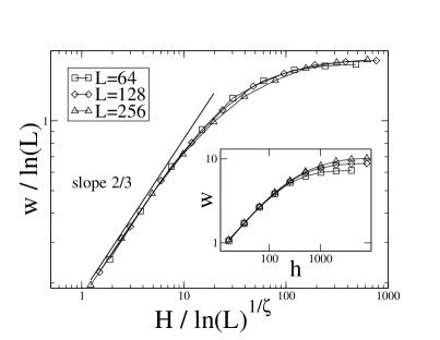
Figure 2: Scaling plot of the roughness in 2d according to the finite size scaling form (4). The line density is $\rho=0.05$, the roughness exponent is $\zeta=2/3$.

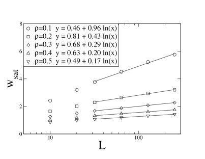
Figure 3: Saturation roughness as a function of the system width with fits of the form $y=A+B\,{\mathrm{l}n}(L)$.

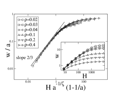
Figure 4: Scaling plot for the roughness in 2d according to the scaling form (5). The system size is fixed at $L=256$.

We computed the ground states of a large number of disorder realizations (up to $10^{3}$) for various values of $L$, $H$ and $\rho$ and produced scaling plots for fixed line density $\rho$ according to the suggested size scaling form (4). We found a good data collapse for all values of $\rho$ that we checked ($\rho=0.05$,…,$0.5$). In Fig. 2 we show the data collapse for $\rho=0.05$. This particular value results in the best data collapse for the achieveable system sizes.

We estimated the saturation roughness $w_{\rm sat}=\lim_{H\to\infty}w(H)$ from the flat tail of the roughness curves $w(H)$ and show them in Fig. 3 as a function of $L$ for several values of the line-density $\rho$. The data can be fitted to the form $y=A+B\mathrm{ln}(L)$ again reflecting the collective super-rough scaling of the roughness in 2d. The slope $B$ of the data sets decreases as $\rho$ increases while the constant part $A$ does not vary much. This leads to the strengthening of finite size effects with increasing $\rho$.

The crossover from single-line to multi-line scaling takes place when $H^{\zeta}\sim a$, where $a$ is the average line-to-line distance $a=1/\rho$ in 2d. For fixed but large lateral system size $L$ the scaling form (4) predicts

$$w\approx a\cdot\tilde{g}_{2d}(H/a^{1/\zeta})$$ (5)

where the scaling function $\tilde{g}_{2d}(x)$ has the asymptotic behavior $\tilde{g}_{2d}(x)\sim x^{\zeta}$ for $x\ll 1$ and $\tilde{g}_{2d}(x)\sim const.$ for $x\gg 1$. Fig. 4 shows the corresponding data collapse of the roughness data that we computed. Note that the height has been also rescaled with a factor of $1-1/a$ to account for the limit $\rho\rightarrow 1$.

IV Roughening in 3d

In this section we present our numerical results and the corresponding scaling laws obtained for the 3d case. If the observations we made in the last section could be carried over to the 3d case, one would expect 2 regimes: One for small heights $H$, in which the transverse fluctuations of the lines are still much smaller than the average line-to-line distance $a=1/\rho^{1/2}$ in 3d; and one for large $H$, in which the line roughness is restricted due to collective effects. Only in the case our line system would also for 3d fall into the same universality class as a 3d elastic medium (this is, as we have shown the case in 2d), one would expect $w_{\rm sat}\propto\sqrt{\ln L}$ elastic3d ; elnum3d .

However, surprisingly we find i) three regimes instead of two (c.f. the data shown in Fig. 5), and ii) $w_{\rm sat}\propto L$, i.e. the size of the transverse fluctuations is not restricted by the presence of a large number of other lines but only by the lateral system size. Apparently in 3d the lines become transparent to each other, and the wandering of any line to the transverse direction does not induce collective behavior.

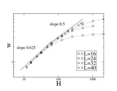
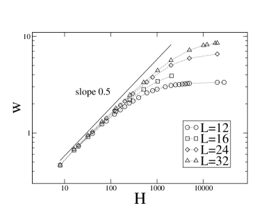
Figure 5: Data for the roughness $w$ as a function of the height $H$ for different transverse system sizes $L$ and two densities: $\rho=0.005$ (top) and $\rho=0.4$ (bottom). In the low density limit (top) the crossover from single line to collective behavior is visible - indicated by the two straight lines with slope $0.625$, the sinle line roughness exponent, and $0.5$, respectively. In the high density limit the crossover from collective line behavior (indicated by the straight line with slope $0.5$) to the saturation regime is visible. The data points are averaged over 100-1000 samples.

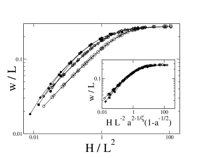
Figure 6: Scaling plot of the roughness in 3d according to the finite size scaling form (6) for different line densities $\rho=0.1$ (filled symbols), $0.2$ (bold) and $0.4$ (empty) for system sizes $L=16$ (ovals), $24$ (squares) and $32$ (diamonds). The inset shows data collapse according to the scaling form (9).

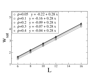
Figure 7: Saturation roughness as a function of the system width with linear fits to the data points.

The three regimes that we find can be characterized as follows: 1) A single line regime for $H\ll a^{1/\zeta}$ in which the roughness behaves as in the the one-line case: $w\propto H^{\zeta}$. 2) An intermediate regime for $a^{1/\zeta}\ll H\ll L^{2}$ in which the roughness increases as $H^{1/2}$, which is identical to the behavior of random walks. Between the two regimes one can see a cross-over that can be shown to be related to the entropic repulsion of the lines. Recall that this leads in 2d asymptotically to collective effects, but here the consequences are different. 3) The saturation regime for $H\gg L^{2}$ in which the roughness saturates at the lateral system size: $w\approx L$. In the following we support this central result with the data we obtained from our ground state calculations for the 3d system and derive the appropriate scaling forms for the different regimes.

In Fig. 6 we show our results for the roughness in 3d in the crossover region from the intermediate or multi-line regime to the saturation regime. We show data for three different line density values, but we have also data for other values, and they all fit well into the scenario that we propose now). The finite size scaling plots yield an excellent data collapse using the scaling form:

$$w=L\cdot g_{3d}^{(a)}(H/L^{2})\;.$$ (6)

The scaling function $g_{3d}^{(a)}(x)$, which still depends on $a$, or the line density $\rho=1/a^{2}$, has the following asymptotic behavior: $g_{3d}^{(a)}(x)\propto x^{1/2}$ for $x\to 0$ and $g_{3d}^{(a)}(x)=const.$ for $x\to\infty$.

The first crucial observation here – and the essential difference to the 2d case – is that in the limit $L\to\infty$ the roughness is not significantly restricted by the presence of the other lines but approaches a value proportional to the lateral system size. Actually, as we see from the plot of the saturation roughness as a function of $L$ shown in Fig. 7 that $w_{\rm sat}=\lim_{H\to\infty}w(L,a)=0.28\cdot L+c_{a}$, where $c_{a}$ is a small constant that varies only slightly with $a$. This variation with $a$ is a boundary effect: The free boundary conditions act effectively in a repulsive way on the lines that competes with the steric inter-line repulsion. Therefore systems with a lower line density show smaller transverse line fluctuations than those with a higher density.

The second crucial observation is that the roughness of the lines in the intermediate regime grows like $H^{1/2}$, i.e. they have a roughness exponent that is smaller than the single line value of $\zeta=0.625$ and is identical to the value for simple random walks. Although the actual line configuration is constructed in a highly non-trivial manner via a global criterion, namely the computation of the global $N$-line ground state, their universal geometric properties appear to be similar to that of random walks.

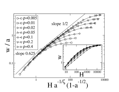
Figure 8: Scaling plot for the roughness in 3d in the crossover region from single to multi-line behavior. The system size is $L=32$. The inset shows the original, unscaled data.

The density dependence of the scaling functions $g_{3d}^{(a)}(x)$ can be worked out by matching it with the scaling form for the single- to multi-line regime. Here the relevant length scale in the $H$-direction is $a^{1/\zeta}$, and in analogy to the 2d case we expect for $L\gg a$ the $L$-independent scaling form

$$w=a\cdot\tilde{g}_{3d}(H/a^{1/\zeta})$$ (7)

with the asymptotics $\tilde{g}_{3d}(x)=x^{\zeta}$ for $x\ll 1$ and $\tilde{g}_{3d}(x)=x^{1/2}$ for $x\gg 1$. In Fig. 8 we show the corresponding scaling plot for the data that we obtained from our calculations. Hence we get the expected single line behavior $w\sim H^{\zeta}$ when $H\ll a^{1/\zeta}$, and we obtain

$$w=a^{1-(1/2\zeta)}H^{1/2}\quad{\rm for}\quad w\ll L\quad{\rm and}\quad H\gg a^{1/\zeta}\;.$$ (8)

From this the natural scaling variable for the crossover region from the intermediate regime (where $w$ should be described by (8)) to the saturation regime (where $w$ should be proportional to $L$ according to (6)) appears to be $a^{1-(1/2\zeta)}H^{1/2}/L$ or $H/a^{1/\zeta-2}L^{2}$, which implies that (6) can be rewritten as

$$w=L\cdot g_{3d}(H/a^{1/\zeta-2}L^{2})\quad{\rm for}\quad H\gg a^{1/\zeta}\;.$$ (9)

with $g_{3d}(x)=x^{1/2}$ for $x\to 0$ and $g_{3d}(x)=0.28$ for $x\to\infty$ (see the inset in Fig. 6). As in 2d, for high line densities $\rho>0.1$ ($a\lesssim 3$) one has to take into account the limiting case $\rho=1$ where lines fill all parallel lattice bonds resulting zero roughness. This limit can be incorporated into (9) by rescaling $H$ by $1/(1-\rho)$.

At this point we would like to stress that the random walk like scaling is not related to the actual distance at which the lines touch or cross each other (and are in some cases continued randomly). Both in 2d and in 3d the typical length scale $s$ between two consecutive intersection points on one line is much larger then the length scale $\xi$ for the crossover from single line to collective behavior and its divergence with the line average distance $a$ is much stronger. This can be seen in Fig. 9, where we show scaling plots for the average length of line segments $s$ between two crossings, from which one conludes that $s$ scales with $a$ as $a^{2.6}$ in 2d (compared to $a^{1.5}$ for the crossover lenght scale $\xi$) and $a^{3.2}$ in 3d (compared to $a^{1.6}$ for $\xi$). This also demonstrates that the lines do not behave like independent random walkers in 3d but reflect the effect of a steric repulsion that tends to avoid random crossings between them (visible in 2d and in 3d).

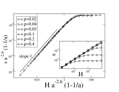
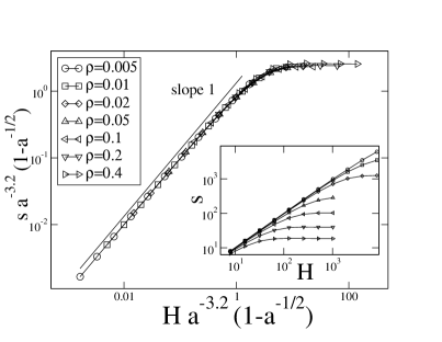
Figure 9: Scaling plots for the length of line segments $s$ between two crossings (a) in 2d, the system size is $L=256$ and (b) in 3d, the system size is $L=32$. The insets show the original, unscaled data.

The main result of calculations for the 3d system is that the lines with only hard core repulsion can transverse the whole system, in marked difference to the 2d case. One can visualize this result also by looking at the disorder averaged position of the center of mass of the individual lines (which is $\overline{r}$ as defined under (3)). In 2d they constitute a regular array on the base line with lattice spacing $a$. In 3d, as we show in Fig. 10, the still constitute a regular array, but it concentrates, with increasing height, more and more in the central region of the basal plane of the system. In the limit $H\to\infty$ the average center of mass position of each individual line will be exactly at the center of the system since nothing restricts it from transversing the system from one side to the other.

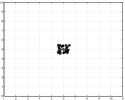
Figure 10: Average positions of center of masses of lines with fixed starting points. From left: H=10, H=100, H=1000. Note that the center of mass position is averaged over the disorder, here 1000 samples.

V Weak and anisotropic disorder distribution

Next we check the robustness of the universal scaling forms in Eqs. (4), (5), and (6) against a more general disorder distribution. The random energy $e_{i}$ is distributed in $[0,\delta]$ with $\delta>0$ if the bond $i$ is in the transverse direction while in $[1-\epsilon,1+\epsilon]$ with $0\leq\epsilon\leq 1$ if the bond is in the longitudinal direction. The disorder distributions on the transverse bonds and the longitudinal ones are thus different unless $\epsilon=1$ and $\delta=2$. Moreover, as $\epsilon$ becomes smaller, the energies on the longitudinal bonds are more highly concentrated around $1$ implying weaker disorder.

Figure 11: Data collapse of the scaled roughness $w/\ln L$ vs. the scaling variable $H(\epsilon/\delta)^{\nu}/(\ln L)^{1/\zeta}$ of interacting lines in the 2d lattice of size $L\times H$ with $L=16$, $32$, $64$, and $128$ and the line density $N/L=1/16$. The parameters $\epsilon$ and $\delta$ are chosen as in the legend. The exact wandering exponent $\zeta=2/3$ barabasi95 and the fitting value $\nu\simeq 0.8(1)$ are used for the scaling variable. The inset is the plot of the roughness $w$ vs. $H$ for $L=64$. Dependence of $w$ on $\epsilon$ and $\delta$ is shown before the roughness saturates.

When $\epsilon=0$ or $\delta^{-1}=0$, the lines are flat, i.e., $w=0$ because there is no energy reduction that compensates for the energy cost accompanying a transverse fluctuation. On the other hand, when $\epsilon=1$ and $\delta=2$, the lines are rough and exhibits the universal scaling behavior shown previously. Therefore it would be desirable to find the boundary between such distinct two limits in the ($\epsilon,\delta$)-plane. We computed the roughness for the generalized disorder distribution with various values of $\epsilon$ and $\delta$, which is shown in Figs. 11 (2d) and 12 (3d). We consider for 2d systems with the fixed line density $N/L=1/16$. In 3d, a single line is studied to sort out the effect of $\epsilon$ and $\delta$ on the roughness scaling in Eqs. (4), (5), and (6) more clearly. The roughness shows the same scaling behaviors as in the previous sections except for the dependence on $\epsilon$ and $\delta$ before it saturates. It implies that interacting lines are rough for nonzero $\epsilon$ and $\delta^{-1}$ and that the scaling behaviors in Eqs. (4), (5), and (6) are universal with respect to the variations of the disorder distribution used here.

Figure 12: Data collapse of the scaled roughness $w/L$ vs. the scaling variable $H(\epsilon/\delta)^{\nu}/L^{1/\zeta}$ of one line in the 3d lattice of size $L\times L\times H$ with $L=8$, $16$, and $32$. The wandering exponent $\zeta=0.625$ barabasi95 ; lassig98 is used and the exponent $\nu$ is found to be $0.68(8)$. The inset is the plot of the roughness $w$ vs. $H$ for $L=8$.

The dependence of the roughness on $\epsilon$ and $\delta$ before it saturates is rooted in the crossover behavior around the point $(\epsilon,\delta^{-1})=(0,0)$. As $(\epsilon,\delta^{-1})$ deviates from $(0,0)$, a line roughens ($w>0$), if the reduction of the longitudinal-bond energy obtained by the transverse fluctuation is larger than the accompanying energy cost. By comparing the energy reduction and cost accompanying the transverse fluctuation, one can get the crossover (“Larkin”) length scale for $H$, $\xi_{H}$. For a given line $i$, the typical fluctuation or the standard deviation of the sum of the energies on the longitudinal bonds, $E_{i,\parallel}=\sum_{z}e_{\parallel}({\bf r}_{i}(z))$, is given by $\epsilon\sqrt{H}$, which corresponds to the average reduction of $E_{i,\parallel}$ achieved by a transverse fluctuation. On the other hand, the line chooses the position where the cost is minimum among $H$ possible ones ($1\leq z\leq H$) to fluctuate in the transverse direction. The cost on the average is equal to the average minimum value of $H$ independent random variables each of which is distributed uniformly in $[0,\delta]$, which is given by $\delta/(H+1)$ gumbel58 . Comparing the energy reduction and cost, one finds the characteristic length scale $\xi_{H}$ as

$$\xi_{H}\sim\left(\frac{\epsilon}{\delta}\right)^{-2/3},$$ (10)

such that the roughness $w$ is zero for $H\ll\xi_{H}$ and non-zero, increasing as $H^{\zeta}$ for $H\gg\xi_{H}$. From the numerical data and the above argument, the roughness in 2d and 3d for the generalized disorder distribution used here can be represented as

$$w\sim\left\{\begin{array}[]{ll}0&(\frac{H}{\xi_{H}}\ll 1),\\ \left(\frac{H}{\xi_{H}}\right)^{\zeta}&(1\ll\frac{H}{\xi_{H}}\ll[w_{\rm sat}(L)]^{1/\zeta}),\\ w_{\rm sat}(L)&(\frac{H}{\xi_{H}}\gg[w_{\rm sat}(L)]^{1/\zeta}),\end{array}\right.$$ (11)

with the usual roughness exponents and saturation roughness scalings according to the dimension. The crossover scaling function between the transient regime and the stationary state is represented in terms of the scaling variable $H/\xi_{H}/(w_{\rm sat}(L))^{1/\zeta}$, which is shown in Figs. 11 and 12 with the fitting value for $\nu$ in $\xi_{H}\sim(\epsilon/\delta)^{-\nu}$ being $0.8(1)$ (two dimension) and $0.68(8)$ (three dimension), the latter being in rather good agreement with 2/3. The derivation of (10) corresponds to comparing elastic energy to the pinning energy in a conventional derivation of the Larkin length. Obviously in two dimensions one should be more careful while simply equating the costs of tranverse bonds to the elastic energy of the line and the costs of longitudinal bonds to the strength of a pinning potential.

VI Conclusions

In this work we have considered the collective effects arising from the interaction of “forests” of directed polymers, in the presence of quenched randomness. In both 2d and 3d this is marked by a cross-over from individual, rough lines to a “collective” regime with a system-size dependent roughness $w$. In 2d, our studies augment earlier work on similar systems using fixed line densities. The approach is based on a mapping of the problem to the minimal matching problem of combinatorial optimization, and the essential point of our model(s) is that the density of lines is a free parameter. In this, we consider the cross-over to the asymptotic collective roughness as a function of the parallel and perpendicular disorder strengths.

In 3d, perhaps more importantly, it is found that the generally expected logarithmic roughening is absent: while (scalar) models of weakly perturbed elastic manifolds do exhibit logarithmic roughness scaling this is not the case here. An ensemble of directed polymers with hard-core interactions exhibits almost “trivial” roughening, with a random-walk -like scaling picture. There is a crucial difference between two and three spatial dimensions even within the confines of the same microscopic model. An ensemble of directed polymers with locally repulsive interactions is thus proven to be different from other approaches using mappings to e.g. higher-dimensional manifolds that do exhibit logarithmic correlations elnum3d . It is worth noting that this does not follow from a “profileration of dislocations” in a vortex lattice, but from the absence of collective behavior.

A rather random but likewise potentially very important consequence of the same is that in 3d the lines entangle - the topological state becomes highly non-trivial such that it might be useful to describe it in terms of knot-theoretical means entangle ; Nechaev . Such concomitant geometrical structures are again absent in models for 3d elastic media. In this case, the description of barriers and excitations still remains to be done including the effect of the entanglement on both.

- (1) For a review see G. Blatter et al., Rev. Mod. Phys. 66, 1125 (1994).
- (2) T. Nattermann, Phys. Rev. Lett. 64, 2454 (1990); T. Giarmachi and P. Le Doussal, Phys. Rev. Lett. 72, 1530 (1994); and Phys. Rev. B 52, 1242 (1995).
- (3) M. P. A. Fisher, Phys. Rev. Lett. 62, 1415 (1989); D. S. Fisher et al, Phys. Rev. B 43, 130 (1991).
- (4) D. A. Huse and C. L. Henley, Phys. Rev. Lett. 54, 2708 (1985); M. Kardar, Phys. Rev. Lett. 55, 2924(C) (1985); D. A. Huse, C. L. Henley and D. S. Fisher, Phys. Rev. Lett. 55, 2924 (1985);
- (5) B. M. Forrest and L. H. Tang, Phys. Rev. Lett. 64, 1405 (1990); J. M. Kim, M. A. Moore, A. J. Bray, Phys. Rev. A 44, 2345 (1991).
- (6) J. Toner and D. P. DiVicenzo, Phys, Rev. B 41, 632 (1990); T. Hwa and D. S. Fisher, Phys. Rev. Lett. 72, 2466 (1994).
- (7) C. Zeng, A. Alan Middleton, and Y. Shapir, Phys. Rev. Lett. 77, 3204 (1996); S. Bogner, T. Emig and T. Nattermann, Phys. Rev. 63 174501 (2001).
- (8) T. Giamarchi and P. Le Doussal, Phys. Rev. B 52, 1242 (1995);
- (9) D. McNamara and A. Alan Middleton, Phys. Rev. B 60 10062 (1999).
- (10) V. Petäjä, M. Alava, and H. Rieger, Int. J. Mod. Phys. C 12, 421 (2001).
- (11) M. Alava, P. Duxbury, C. Moukarzel, and H. Rieger, in Phase Transitions and Critical Phenomena, Vol. 18, edited by C. Domb and J.L. Lebowitz (Academic Press, 2000); A. Hartmann and H. Rieger, Optimization Algorithms in Physics (Wiley VCH, Berlin, 2002).
- (12) A.-L. Barabasi and H.E. Stanley, Fractal Concepts in Surface Growth (Cambridge University Press, Cambridge, 1995).
- (13) E.J. Gumbel, Statistics of Extremes (Columbia University Press, New York, 1958).
- (14) M. Lässig, Phys. Rev. Lett. 80, 2366 (1998).
- (15) V. Petäjä, M. Alava, and H. Rieger, Europhys. Lett. 66, 778 (2004).
- (16) R. Bibkov and S. Nechaev, Phys. Rev. Lett. 87, 150602 (2001); S. K. Nechaev, Statistics of knots and entangled random walks, (World Scientific Publishing ,1996).