Characterizing the network topology of the energy landscapes of atomic clusters

Abstract

By dividing potential energy landscapes into basins of attractions surrounding minima and linking those basins that are connected by transition state valleys, a network description of energy landscapes naturally arises. These networks are characterized in detail for a series of small Lennard-Jones clusters and show behaviour characteristic of small-world and scale-free networks. However, unlike many such networks, this topology cannot reflect the rules governing the dynamics of network growth, because they are static spatial networks. Instead, the heterogeneity in the networks stems from differences in the potential energy of the minima, and hence the hyperareas of their associated basins of attraction. The low-energy minima with large basins of attraction act as hubs in the network. Comparisons to randomized networks with the same degree distribution reveals structuring in the networks that reflects their spatial embedding.

I Introduction

In recent years, characterizing the energy landscape of a system in order to gain a better understanding of its behaviour has become an increasingly popular research approach,Wales (2003) with many applications in the fields of protein folding,Bryngelson et al. (1995) clusters and supercooled liquids.Stillinger and Weber (1984); Stillinger (1995); Debenedetti and Stillinger (2001) For example, a common explanation for how proteins are able to overcome the Levinthal paradoxLev and fold to their native state on biologically reasonable time scales is in terms of a funnel-like energy landscape.

Here, we want to take a somewhat different approach and focus not on the relationship between the landscape and a system’s behaviour, but on some of the fundamental properties of potential energy landscapes. For example, the number of minima increases exponentially with system size Stillinger and Weber (1982); Stillinger (1999); Tsai and Jordan (1993) and the size scaling for higher-order saddle points has also been obtained.Doye and Wales (2002); Shell et al. (2004); Wales and Doye (2003) It is also known that the distribution of minima should be a Gaussian function of the potential energy.Sciortino et al. (1999); Büchner and Heuer (1999)

In this paper we seek to provide fundamental new insights into the structural organization, and particularly the connectivity, of an energy landscape. To achieve this we first map the landscape onto a network, and then analyse the topology of this network for a series of small clusters for which complete networks can be obtained. A brief report of some of this work has already appeared.Doye (2002)

Our analysis of these networks is heavily influenced by the literature on complex networks.Strogatz (2001); Albert and Barabási (2002); Barabási (2002); Bornholdt and Schuster (2003); Dorogovtsev and Mendes (2003); Newman (2003a) The recent interest in this area was in part sparked by the seminal paper of Watts and Strogatz,Watts and Strogatz (1998) who showed that many real-world networks have features that are typical both of a lattice (the presence of local order) and of a random graphErdős and Rényi (1959, 1960) (short average separations between the nodes), and introduced a ‘small-world’ network model that could represent both these features. Subsequently, it has been shown that many networks also have a probability distribution for the number of connections to a node (in network parlance, the degree distribution) that has a power-law tail. Such ‘scale-free’ networksBarabási and Albert (1999) have been found in an impressively diverse range of fields, including astrophysics,Hughes et al. (2003) geophysics,Baiesi and Paczuski (2004) information technology,Albert et al. (1999) biochemistry,Jeong et al. (2000, 2001) ecologyDunne et al. (2002) and sociology.Liljeros et al. (2001)

The paper is organized as follows. In Section II we explain how energy landscapes can be described in terms of networks. In Section III we present a detailed characterization of these networks. This analysis initially focusses on whether the networks show small-world and scale-free behaviour, before going on to look at more subtle features of these networks. Then, in Section IV we discuss the implications of our results for understanding the dynamics on complex energy landscapes.

II Energy landscapes as networks

To model an energy landscape as a network one must first decide on a definition both of a state of the system and how two states are connected. The states and their connections will then provide the nodes and edges of the network. For systems with continuous degrees of freedom, perhaps the most natural way to achieve this is through the ‘inherent structure’ mapping of Stillinger and Weber.Stillinger and Weber (1982, 1984) In this mapping each point in configuration space is associated with the minimum (or ‘inherent structure’) reached by following a steepest-descent path from that point. This mapping divides configuration space into basins of attraction surrounding each minimum on the energy landscape, and is illustrated for a model two-dimensional energy landscape in Fig. 1.

For systems with large numbers of degrees of freedom, the energy landscape is an extremely complicated multi-dimensional function. The inherent structure approach provides a way of dealing with this complexity by breaking the landscape up into more manageable pieces. For example, good approximations to the partition function of a basin of attraction and to the rates of transitions between two basins can be obtained within the harmonic approximation (and if necessary with additional anharmonic corrections), thus allowing thermodynamic and dynamic properties of a system to be calculated.Wales (2003)

The inherent structure approach also provides a natural partition for the dynamics of a system. At sufficiently low temperature, the system will spend most of its time oscillating within a basin of attraction surrounding a minimum with occasional hops between basins along a transition state valley.Tx This interbasin dynamics can then be represented as a walk on a network, whose nodes correspond to the minima and where edges link those minima that are directly connected by a transition state (a first-order saddle point). Such a network is illustrated for the model surface in Fig. 1, and we will term them inherent structure networks.

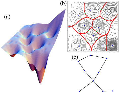
Figure 1: (Colour online). (a) A model two-dimensional energy surface. (b) A contour plot of this surface illustrating the inherent structure partition of the configuration space into basins of attraction surrounding minima. The basin boundaries are represented by thick lines, and the minima and transition states by dots. (c) The resulting representation of the landscape as a network.

In chemistry such networks are often called reaction graphs, and have been used to analyse isomerization in small molecules and clusters. In these applications, each permutational isomer of a structure is usually considered separately. For example, in Ref. Taketsugu and Wales, 2002 the reaction graph connecting the eight permutational isomers of water dimer is depicted. Such knowledge is for example important for understanding the pattern of splittings that results from tunnelling between these isomers.

For an atomic cluster with a single atom type the number of permutational isomers of a minimum is $2N!/h$ where $h$ is the order of the point group of that minimum. This factor makes consideration of the network with a node for each permutational isomer unfeasible for all but the smallest sizes. For example, for a 7-atom Lennard-Jones (LJ) cluster the four geometrically distinct minima give rise to 8904 permutational isomers, but for LJ₁₄ the 4196 geometrically distinct minima give rise to $6.68\times 10^{14}$ permutational isomers. Hence, here we consider the network where each geometrically-distinct minimum is represented by a single node. Indeed, this approach is perfectly reasonable, because one is usually only interested in the structure of the system, and not in the permutational order. The network we consider here will also be unweighted, i.e. we are only interested in whether two minima are connected, and not in the weight, however defined, of this connection.

Table 1: Properties of the energy landscapes and inherent structure networks for LJ_N for $N=7-14$. $n_{\rm min}$ is the number of minima; $n_{\rm ts}$ is the number of transition states; $n_{\rm edges}$ is number of edges in the network; $p$ is the average probability of an edge between any two nodes; $\langle k\rangle$ is the average degree; $k_{\rm max}$ is the maximum degree; $l_{\rm ave}$ is the average separation between nodes; $r$ is the radius of the network; $d$ is the diameter of the network; $C_{1}$ and $C_{2}$ are different definitions of the clustering coefficient; and $r_{k}$ and $r_{E}$ are the assortativity coefficientsNewman (2002, 2003b) with respect to the degree and the potential energy of the minimum, respectively. The uncertainties in the last two quantities have been calculated using the jack-knife method.

$N$	$n_{\rm min}$	$n_{\rm ts}$	$n_{\rm edges}$	$p$	$\langle k\rangle$	$k_{\rm max}$	$l_{\rm ave}$	$r$	$d$	$C_{1}$	$C_{2}$	$r_{k}$	$r_{E}$
7	4	12	5	0.833	2.50	3	1.167	1	2	0.750	0.833	$-0.667\pm 0.359$	$-0.559\pm 0.321$
8	8	42	16	0.571	4.00	6	1.464	2	3	0.621	0.604	$-0.441\pm 0.236$	$-0.379\pm 0.250$
9	21	165	74	0.352	7.05	15	1.714	2	3	0.504	0.607	$-0.287\pm 0.130$	$-0.114\pm 0.114$
10	64	635	359	0.178	11.22	34	2.146	3	4	0.421	0.519	$-0.018\pm 0.058$	$0.080\pm 0.054$
11	170	2424	1623	0.113	19.09	86	2.135	3	4	0.292	0.362	$-0.081\pm 0.024$	$0.101\pm 0.026$
12	515	8607	5854	0.044	22.73	281	2.300	3	5	0.183	0.306	$-0.100\pm 0.009$	$0.097\pm 0.013$
13	1509	28756	20708	0.018	27.45	794	2.394	3	5	0.110	0.260	$-0.097\pm 0.003$	$0.072\pm 0.007$
14	4196	87219	61085	0.007	29.12	3201	2.325	3	6	0.052	0.249	$-0.066\pm 0.001$	$0.082\pm 0.004$

In the first instance, self-connections and multiple edges are also excluded, even though there are transition states that mediate degenerate rearrangements between permutational isomers of the same minimum, and there can be more than one geometrically distinct transition state connecting two particular minima. As a consequence of these exclusions the number of edges in our networks, so defined, is roughly 30% less than the total number of transition states for the larger clusters (See Table 1). We exclude self-connections, both because we are not interested in permutational order, and because degenerate rearrangements make no contributions to the structural dynamics, and multiple edges because we are not so much interested in the number of connections between two minima, but just whether they are connected. Besides, if we were concerned with the number of connections it would not be as simple as counting the number of geometrically distinct transition states that connect the two minima because of symmetry factors. The number of versions of a transition state that connects to a minimum for a non-degenerate rearrangement is given by the factor $h_{\rm min}/h_{\rm ts}$, i.e. the ratio of the orders of the point groups of the minimum and the transition state.Wales (2003)

The properties of these types of networks have effectively been studied before, albeit in a directed form where the links have been weighted by the rate of transition from one minimum to another at a particular temperature.Berry and Breitengraser-Kunz (1995); Miller et al. (1999); Doye and Wales (1999); Wales (2002) This approach leads to a rate matrix from which an exact solution of the interminimum dynamics of the system can be obtained in terms of the eigenvalues and eigenvectors of this matrix using a master equation method. However, in all these applications the emphasis was on the resulting dynamics and not on the topological structure of the networks. Moreover, because the focus was the dynamics of a particular transition and not the global dynamics, most of the networks studied were incomplete.

We should mention three other studies that have sought to characterize the connectivity of configuration space in terms of complex networks.Amaral et al. (2000); Scala et al. (2001); Wuchty (2003) The first was of a two-dimensional lattice polymer, where each discrete configuration was a node in the network and configurations were linked to those that could be obtained by the application of a single elementary move using a move set of corner flips and “crankshaft” rotations.Amaral et al. (2000); Scala et al. (2001) The second was of RNA considered at the secondary structure level, where a node corresponded to those configurations that had the same map of contacts between nucleotides and nodes were linked to those that could be obtained by an elementary change in the contact map.Wuchty (2003) The main differences between these networks and our own is in the discrete, rather than continuous, nature of the configuration space and the definition of a state—there is no equivalent of the inherent structure mapping that groups configurations into a single state (or basin). We will discuss the consequences of these differences later in the paper, when we report the properties of the inherent structure networks. The third study, which examined the connectivity of the conformation space of polypeptides,Rao and Caflisch (2004) is in a much more similar spirit to the current work, because the space is continuous and connections have a dynamical basis. Given the much larger size of the configuration space than in the current study, a more coarse-grained picture of the landscape is required. Rao and Caflisch probe the connections between free energy minima defined through structural order parameters that assign a secondary structure character to each amino acid. The sampling of the landscape is not complete, but instead based on long molecular dynamics simulations at a temperature near to the folding transition. The properties of these networks are much more similar to the present networks.

III Network Properties

We chose to characterize the inherent structure networks of a series of Lennard-Jones clusters, whose potential energy is given by

$$V=4\epsilon\sum_{i<j}\left[\left(\sigma\over r_{ij}\right)^{12}-\left(\sigma\over r_{ij}\right)^{6}\right],$$ (1)

where $\epsilon$ is the pair well depth and $2^{1/6}\sigma$ is the equilibrium pair separation. We concentrate on small systems for which we are able to characterize the energy landscape completely, because we are interested in the global topology of the complete inherent structure network. We choose to study clusters, rather than a bulk system to avoid complications associated with boundary conditions. For clusters we do not have to worry about the density dependence of the networks. Moreover, for systems that are small enough for the complete inherent structure network to be sampled, periodic boundary conditions represent a significant perturbing constraint on the system, and so do not provide an accurate representation of a bulk system. By contrast, small LJ clusters are interesting systems in their own right, whose structural, thermodynamic and dynamic properties have been well characterized.

A (near-)complete sampling of the relevant stationary points of LJ_N up to $N$=13 had previously been obtained in a work looking at the scaling behaviour of the numbers of stationary points.Doye and Wales (2002) In addition we generated samples of minima and transition states for LJ₁₄.

Here, we quickly summarize the approach used. It is an iterative procedure whereby starting from each minima in our sample we perform a series of transition state searches. We then step off any new transition states along the direction of negative curvature to find the connecting minima. More transition state searches are then performed from any new minima. This procedure is repeated until the number of transition states appears to have converged with respect to increasing numbers of searches. However, to find all the transition states we also have to perform searches for second-order saddle points starting from the transition states and minima. From these second-order saddle points we then repeatedly perform transition state searches. With this additional tool the number of transition states increases significantly and does appear to converge to the true total, although of course there is no proof of this.

The number of minima and transition states found by this procedure for each cluster size are given in Table 1. The factor that limits the size for which such complete stationary point samples can be generated is not so much the number of stationary points, but the huge number of searches that need to be performed to achieve convergence. We were able to map out the complete inherent structure networks for all clusters up to $N$=14. The network data is available online.ISN

There is a theoretical expectation that the number of minima and transition states scale with size as Stillinger and Weber (1982); Stillinger (1999); Doye and Wales (2002)

$$n_{\rm min}=e^{\alpha N}\qquad\hbox{and}\qquad n_{\rm ts}=aNe^{\alpha N}$$ (2)

where $\alpha$ and $a$ are constants. These forms are based on the assumption of a bulk system (i.e. large $N$ and no surface) that can be divided up into independent equivalent subsystems. Hence, one should not expect these forms to hold too precisely for small clusters. Expressions for the number of higher-order saddle points can also be derived.Shell et al. (2004); Wales and Doye (2003) Based on the Hessian index for which the number of stationary points is a maximum, a value of $a$=2 appears appropriate for clusters.Wales and Doye (2003)

In network parlance, the number of connections to a node is called the degree and denoted by $k$. Taking the above forms for $n_{\rm min}$ and $n_{\rm ts}$ as appropriate and ignoring for the moment that not all transition states give rise to edges in the networks (because of our exclusion of multiple edges and self-connections), one expects that the average degree for our networks should follow

$$\langle k\rangle\approx{2n_{\rm ts}\over n_{\rm min}}=2aN={2a\over\alpha}\log n_{\rm min},$$ (3)

i.e. $\langle k\rangle$ should scale linearly with the size of the clusters, or logarithmically with the size of the network. It follows that $p$, the fraction of all possible edges in the network that are actually connected is given by

$$p\approx{2n_{\rm ts}\over n_{\rm min}(n_{\rm min}-1)}={2aN\over e^{\alpha N}-1}={2a\log n_{min}\over\alpha(n_{\rm min}-1)}.$$ (4)

Hence the networks should become more sparse as they increase in size.

In line with these theoretical expectations, significant increases of $\langle k\rangle$ with $N$ and decreases of $p$ with $N$ are apparent from Table 1. As we will be comparing networks generated from clusters of different size, it should be remembered that these basic features of the networks are changing.

III.1 Small world properties

One of the key properties when deciding whether a network behaves as a ‘small world’ is the average separation between nodes, $l_{\rm ave}$. More precisely, for each pair of nodes in the network the shortest pathway between them is found and then the average of the number of steps in these pathways is taken. Values of $l_{\rm ave}$ are given in Table 1 and its dependence on network size is depicted in Fig. 2(a). $l_{\rm ave}$ seems to be growing sub-logarithmically with $n_{\rm min}$, although the growth is non-monotonic—such size effects are typical of small clusters.Jortner (1992)

Two other quantities that reflect the properties of the shortest pathways between nodes are given in Table 1. The diameter, $d$, is the number of steps in the longest such pathway, and the radius, $r$, is the number of steps in the longest pathway for the node for which this is a minimum, i.e. all the other nodes are within $r$ steps of that node. The small values of $l_{\rm ave}$, $r$ and $d$ would suggest that the network is showing the ‘small world’ effect, but a more sophisticated analysis is also needed.

Figure 2: The dependence of (a) the average separation between nodes (in steps) and (b) the clustering coefficient, $C$, on the size of the network, $n_{\rm min}$. The data points for LJ clusters with from 7 to 14 atoms are compared to the values expected for a lattice (Eq. (7)) and an Erdős-Renyi (ER) random graph (Eq. (8)), and to those for randomized (rand) networks with the same degree distribution as the clusters, as labelled. Values of both $C_{1}$ and $C_{2}$ are plotted for the LJ clusters.

The usual approach to decide whether the average separation between nodes shows behaviour typical of a random graph or of a lattice is to test whether $l_{\rm ave}$ is a logarithmic ($\log n_{v}$) or power-law ($n_{v}^{1/d}$ where $d$ is the dimension of the lattice) function of the network size, $n_{v}$, respectively. However, the situation is not that simple for our networks, because both the dimension of configuration space and the average degree increases with the network size. Therefore, to test for lattice-like behaviour we need to compare the network, not to a lattice of fixed dimension and increasing extent, but of fixed extent and increasing dimension. It is of fixed extent because the displacement of an atom that is required to reach the nearest permutational isomer of any minimum should always be of the order of the atomic size.

For a $3N$-dimensional hypercubic lattice with $L$ lattice points along each coordinate direction, the average separation between lattice points is approximately the sum of the average difference for each of the $3N$ coordinates. More specifically,

$$l_{\rm ave}^{\rm latt}={n_{\rm min}\over n_{\rm min}-1}3N\,l_{\rm ave}^{1D},\approx 3N\,l_{\rm ave}^{1D},$$ (5)

where the initial factor is to exclude the zero length paths between a node and itself from the average and

$$l_{\rm ave}^{1D}={1\over L^{2}}\sum_{i,j=1}^{L}|i-j|={(L-1)(L+1)\over 3L}.$$ (6)

Hence $l_{\rm ave}^{\rm latt}=N(L-1)(L+1)/L$.PRL Therefore, the average separation between lattice points scales linearly with the dimension of the system. The dependence of $l_{\rm ave}^{\rm latt}$ on the number of lattice points can be obtained by substituting for $N$ in the above equation using $n_{\rm latt}=L^{3N}$, leading to

$$l_{\rm ave}^{\rm latt}={(L-1)(L+1)\over 3L\log L}\log n_{\rm latt}.$$ (7)

Thus, even in the case of a lattice, the average separation scales logarithmically, because of the increasingly high dimensionality of configuration space.

Figure 3: The cumulative distribution for the number of nodes that have more than $k$ connections. The curves correspond to clusters of different sizes, as labelled. An additional straight line with slope $-(\gamma-1)$, where $\gamma$=2.78, has been plotted to emphasise the power law tail. In the inset the cumulative probability distribution for the 12-, 13- and 14-atom clusters is plotted against $k/\langle k\rangle$, to bring out the universal form of the distribution.

For a random graph

$$l_{\rm ave}^{\rm ER}={\log n_{v}\over\log\langle k\rangle},$$ (8)

so for our networks, if this equation were obeyed we would expect a sublogarithmic scaling with size. In fact, if we substitute the result from Eq. (3) we get

$$l_{\rm ave}={\log n_{\rm min}\over\log\left(2a/\alpha\right)+\log\left(\log n_{\rm min}\right)}$$ (9)

The apparent sublogarithmic behaviour of Fig. 2(a) would suggest that as with the Watts-Stogatz small-world networks, the scaling of $l_{\rm ave}$ is similar to a random graph, but more conclusive evidence in favour of this conclusion comes if we compare Equations (7) and (8) to our data. To apply Eq. (7) a value for $L$ was first obtained using the number of minima for LJ₁₄, which gives $L=1.220$. A much better fit to our data is obtained from the random-graph expression, confirming our initial assessment.

This scaling behaviour may seem somewhat surprising, since the connections between minima are based on the adjacency of the associated basins in configuration space, which would perhaps initially suggest a more lattice-like picture of configuration space. Furthermore, there are no obvious equivalents of the random linkages between distant nodes that cause the small-world behaviour in the Watts-Strogatz networks.Watts and Strogatz (1998) As we will see later, the origin lies elsewhere.

Another feature of many networks is a strong degree of local structure, as measured by the clustering coefficient. The clustering coefficient of node $i$, $c_{i}$, is defined as the probability that a pair of neighbours of $i$ are themselves connected. However, when extending this concept to the whole graph there are two definitions in common usage. The first, $C_{1}$, is simply the probability that any pair of nodes that have a common neighbour are themselves connected,Watts and Strogatz (1998) and the second, $C_{2}$, is the average of the local clustering coefficient: $C_{2}=\sum_{i}c_{i}/N_{\rm min}$. The difference between these two definitions is the relative weight given to nodes with different degree. High degree nodes make a larger contribution to $C_{1}$ because there will be more pairs of nodes that have a high-degree node as a common neighbour, whereas all nodes contribute equally to $C_{2}$. Typically, $C_{1}<C_{2}$ because, as is the case here, higher degree nodes tend to have lower values of $c_{i}$.

Values of $C_{1}$ and $C_{2}$ are given in Table 1 and are compared to that for an Erdős-Renyi random graph ($C^{\rm ER}=p$) in Figure 2(b). It is apparent that the networks for the larger clusters have significantly more local structure than the random graphs. For LJ₁₄ $C_{1}$ and $C_{2}$ are 7.53 and 35.90 times larger than $C^{\rm ER}$, respectively. At small cluster sizes $C\approx C_{\rm ER}$ mainly due to the large values of $p$—there is going to be little difference from a random graph when the network is almost fully connected—but as the networks become more sparse, they show increasing local correlations. This feature of the networks is unsurprising given that the connections are based on adjacency in configuration space.

III.2 The degree distribution

Another very important property of a network is its degree distribution. These distributions are illustrated for our networks in Figure 3. Remarkably, as the size of the clusters increase a clear power-law tail develops. Such networks are typically said to be scale-free, even though the power-law behaviour does not extend back to small values, and so the distribution is not totally invariant to rescaling.Tsa In fact, the initial flat portion of the cumulative degree distributions in Fig. 3 implies that the degree distribution itself has a maximum that lies near to, but below, $\langle k\rangle$. Interestingly, the inset to Fig. 3 suggests that the distribution is tending to a universal form independent of cluster size. The value of the exponent in the power law is 2.78, which is quite similar to other scale-free networks (most are between 2 and 3).

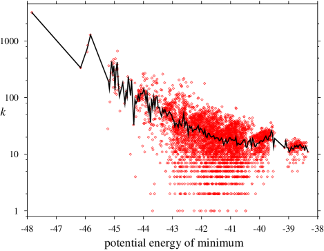
Figure 4: (Colour online). The dependence of the degree of a node on the potential energy of the corresponding minimum for LJ₁₄. The data points are for each individual minimum and the solid line is a binned average.

This result implies that the networks are very heterogeneous, with a few hubs having a very large number of connections, but with most having something near to the average. It also explains the origin of the small-world behaviour, as scale-free networks are known to have very small values of $l_{\rm ave}$. This is because the hubs provide natural conduits for short paths between nodes. In fact, the scaling of $l_{\rm ave}$ with network size can be even slower than for Erdős-Renyi random graphs.Cohen and Havlin (2003); Chung and Lu (2002)

The obvious next question to ask is what features differentiate those minima with large numbers of connections from those with only a few. What is the source of the heterogeneity? Most of the models devised to explain the scale-free properties of networks are dynamic in nature. For example, in Barabasi and Albert’s model it arises from the preferential attachment of new nodes to those with higher degree at each step in the growth process.Barabási and Albert (1999) However, our inherent structure networks are static in nature, and are just determined by the form of the interatomic potential and the number of atoms.

One of the few scale-free models not involving network growth is the fitness model of Calderelli et al., in which each node is assigned a fitness parameter that controls its properties.Caldarelli et al. (2002) For a suitable combination of the distribution of the fitness parameter and the fitness-dependent linking probability, scale-free networks can result.

The most obvious parameter that might control the properties of our nodes is the potential energies of the associated minima. In Figure 4 we show the dependence of the degree of a node on its potential energy for our largest network. There is a strong correlation; the global minimum is the most connected and the degree decays to lower values as the energy increases. This picture is typical of the data for other clusters, and only for LJ₉ and LJ₁₀ is the global minimum not the most highly-connected hub; in fact it is the fifth lowest-energy minimum in both these exceptions. The $k_{\rm max}$ values in Table 1 indicate the highly-connected nature of the hubs. The biggest hub is always connected to more than 50% of the network, and the particularly high value for LJ₁₄ (76%) explains the non-monotonic behaviour of $l_{\rm ave}$ at $N=14$.

Figure 5: (Colour online). (Cumulative) probability distributions for the energy of the minima for LJ₁₄. The distributions are compared to Gaussian forms (dotted lines).

The combination of $k(E)$ illustrated in Fig. 4 with the probability distribution for the potential energy of the minima, $p(E)$, must lead to a power-law tail for $p(k)$, and so this might be one avenue to explain the scale-free behaviour of our networks. Indeed, the form of $p(E)$ has been extensively investigated for a variety of systems, and a physical motivation given for its form. Based on the minima sampled in the liquid state of bulk matter, the distribution of minima has been found to be a Gaussian function of the potential energy.Sciortino et al. (1999); Büchner and Heuer (1999) This form can be justified from the central limit theorem if it is assumed the system can be divided into independent subsystems.Heuer and Büchner (2000)

Our data can also be well-approximated by a Gaussian (Figure 5), however there are deviations in the tail regions. In particular, $p(E)$ decays more slowly than a Gaussian at low energy. This deviation is not so surprising, since the analysis is expected to be most applicable where there is a quasicontinuous distribution of minima, rather than for the more discrete spectrum of minima in the low-energy tail that is associated with the solid form of the clusters. However, this part of the distribution is particularly significant as it determines the properties of the highly-connected minima in the scale-free tail. Indeed, a more detailed analysis shows that the non-Gaussian nature of the low-energy tail of $p(E)$ combines with the faster than exponential increase of $k(E)$ to produce the power-law tail for $p(k)$. However, it is no more clear why these functions should have these precise forms than why $p(k)$ has a power-law tail, so relatively little new physical insight has been obtained.

Probably, a more fruitful way of understanding the heterogeneous nature of the networks is by thinking in terms of the hyperareas of the basins of attraction surrounding a minimum. The high connectivity of the low-energy minima is likely to stem from their large basins of attraction, because this gives them long basin boundaries, and hence the likelihood of a greater number of transition states on these boundaries. Indeed, there is evidence that for LJ₃₈ the basins of attraction rapidly decrease in area with increasing potential energy.Doye et al. (1998) Some statistics are also available for the probability of reaching the global minima of LJ clusters from a random starting point, which provide a direct measure of the relative area of the global minimum.Stillinger and Stillinger (1990); Bytheway and Kepert (1992) These studies indicate that this probability is significantly larger than $1/n_{\rm min}$, and thus that they have large basins of attraction. We intend to pursue this idea further in future work, in particular to examine in detail whether the relationship between basin area and connectivity is as we have suggested.

These ideas lead to a hierarchical picture of the energy landscape, where large basins of attraction are surrounded by smaller basins, which in turn are surrounded by smaller basins, …. A useful way to envisage this heterogeneity of basin areas is by analogy to an Apollonian packing, a two-dimensional example of which is shown in Fig. 6. The initial configuration for this packing is three mutually touching discs. In the interstice between these three discs a new disc is added that itself touches the three discs (the so-called inner Soddy circle). In the three new interstices created, three more discs are added. This procedure is continued iteratively to generate a space-filling packing of discs that is a fractalMandelbrot (1983) of dimension 1.3057.Manna and Herrmann (1991)

As with the basins of attraction that divide configuration space, the discs in the Apollonian packing have a very heterogeneous distribution of areas that is organized hierarchically. In fact, the probability distribution of the areas of the disks is a power-law.Manna and Herrmann (1991) Furthermore, if we consider the Apollonian packing as a network where each disc corresponds to a node and nodes are connected by an edge if the corresponding discs are in contact, then this network has a scale-free degree distribution.Andrade et al. (cond-mat/0406295); Doye and Massen (cond-mat/0407779) Moreover, many of the topological properties of this “Apollonian network” are similar to the inherent structure networks.Doye and Massen (cond-mat/0407779)

Figure 6: An Apollonian packing of disks.

This analogy helps us to understand why our initial intuition—namely, that the inherent structure networks would be lattice-like, because they are based on the adjacency of basins—was wrong. However, there are of course limitations to the analogy. In the Apollonian packing space is filled by an infinite number of discs, whereas configuration space is divided up into a finite number of basins surrounding the minima. Therefore, it’s probably better to compare the ISN to an Apollonian packing where the iterative addition of discs has only been applied a finite number of times.Doye and Massen (cond-mat/0407779)

Having outlined the basic properties of the inherent structure networks, it is useful to compare our results to the other studies looking at the connectivity of configuration space. The scaling behaviour of $l_{\rm ave}$ has been characterized in both Scala et al.’s study of lattice polymersScala et al. (2001) and Wuchty’s analysis of RNA.Wuchty (2003) In Ref. Scala et al., 2001 networks of different size were generated by considering both polymers of different length and with different end-to-end distances. Based on a comparison of $l_{\rm ave}$ to that for a two-dimensional lattice and a random graph, they concluded that there is a crossover to logarithmic scaling for networks of size larger than 100. However, this is the wrong comparison, because the dimension of configuration space is of course, $2N$, where $N$ is the number of monomers in the chain. Instead, the deviation from a power-law scaling is probably due to the effective higher dimensionality of conformation space for the longer polymers. Consistent with this interpretation the degree distribution shows no sign of heterogeneities, but is instead a Gaussian,Amaral et al. (2000) because of the local nature of the move set. Each conformation occupies a similar volume in conformation space.

Wuchty considers only one RNA sequence of a fixed length, but generates networks of different sizes through only including states that are within a certain variable energy of the ground-state. In contrast to our graphs, the networks are therefore incomplete. $l_{\rm ave}$ deviates significantly from that for a random graph, and the degree distribution has a exponential tail.

We would suggest that both these networks are essentially behaving as lattices of high dimensionality, because the local move-sets only allow connections to conformations that are nearby in configuration space, and there is no equivalent to the inherent structure mapping to group conformations into states with widely-differing basin areas.

By contrast, in their study of a protein network Rao and Caflisch found behaviour much more similar to our inherent structure networks with a degree distribution that had a power-law tail and with the low-lying free-energy minima having greater connectivity.Rao and Caflisch (2004) This reflects the conceptual similarities in the network representations noted in Section II and suggests the potential generality of the results we have found here.

III.3 Randomization

Before we look at more detailed properties of the networks, it is useful to have an appropriate random model to which to compare. For example, Dorogovtsev and Mendes have suggested that the values of $C/C^{\rm ER}$ for our inherent structure networks simply reflect the degree distribution and not any additional local structuring.Dorogovtsev and Mendes (2003)

Analytic expressions are available for some network properties of a random ensemble of networks with a given degree distribution.Dorogovtsev and Mendes (2003) However, these do not apply when multiple edges and self-connections are excluded. Instead, we used the switching algorithm to generate the ensembles of random networks.Maslov and Sneppen (2002); Milo et al. (cond-mat/0312028) At each step in this procedure two edges are picked at random, A—B and C—D say, and then rewired to form two new edges, either A—C and B—D, or A—D and B—C. It is evident that this rewiring conserves the degree distribution. It is also straightforward to keep the constraint that there are no multiple edges or self-connections; rewiring steps that would break this constraint are simply not accepted. The procedure is started from the original network, and, after a suitable equilibration period, statistics were recorded. At each step the probability of each edge occurring is followed. From this probability distribution a variety of network properties can be calculated. However, for other properties, e.g. $l_{\rm ave}$, that have to be explicitly calculated for a specific network, averages over 25 independent (as judged by the autocorrelation function of the clustering coefficient) random networks were taken.

Table 2: Some properties of the randomized networks produced from the inherent structure networks by the switching algorithm.Maslov and Sneppen (2002); Milo et al. (cond-mat/0312028)

$N$	$l_{\rm ave}$	$C_{1}$	$r_{k}$	$r_{E}$
8	$1.479$	$0.625$	-0.408	-0.299
9	$1.706$	$0.492$	-0.304	-0.125
10	$2.043$	$0.332$	-0.158	-0.088
11	$2.071$	$0.219$	-0.108	-0.063
12	$2.247$	$0.124$	-0.115	-0.085
13	$2.338$	$0.071$	-0.106	-0.109
14	$2.302$	$0.032$	-0.068	-0.119

Some properties of these randomized networks are given in Table 2. For example, Figure 2(b) shows that although the randomized networks have a significantly higher clustering coefficient than the Erdős-Renyi random graphs, the values for the inherent structure networks are yet still higher. This result disproves Dorogovtsev and Mendes’ assertionDorogovtsev and Mendes (2003) and shows that there are additional sources of local structuring, over and above that due to the degree distribution.

By contrast, in Figure 2(a), which compares $l_{\rm ave}$ for the cluster networks and their randomized versions, only very small differences are apparent, showing that this property primarily reflects the degree distribution of the networks. However, it is noticeable that $l_{\rm ave}^{\rm rand}$ is always systematically smaller, albeit by a small amount, except for LJ₈. This reflects the general correlation between higher clustering and longer path lengths, as seen, for example, in the extremes of the Erdős-Renyi random graphs (low $C$, small $l_{\rm ave}$) and lattices (high $C$, large $l_{\rm ave}$). In a network with higher clustering, edges are ‘wasted’ connecting nodes that are already close, which might have been used to connect distant nodes and hence lower $l_{\rm ave}$ more significantly.

In the following we will only show data for the randomized networks when they show significant differences from the inherent structure networks. Typically, there will only be very small differences for properties related to the shortest paths on the networks, as with $l_{\rm ave}$, but more significant differences appear for properties associated with clustering and network correlations.

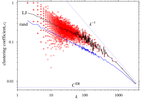
Figure 7: (Colour online). The dependence of the local clustering coefficient of a node on the degree. The data points are for each LJ₁₄ minimum, and the the solid lines are the average values for a given $k$. For comparison, the function $k^{-1}$ and $c(k)$ for the randomized networks and an Erdős-Renyi (ER) random graph have also been plotted.

III.4 Degree dependent properties for LJ₁₄

The extremely heterogeneous nature of our networks is reflected in their scale-free degree distribution. To probe this heterogeneity further, it is also helpful to look at how properties vary from node to node, and particularly how they depend on the degree of a node. We will do this for our largest network, LJ₁₄, but results for smaller networks are similar. Because of the large size of this network, there is often considerable scatter in the data. To make the trends more clear, averages of the properties, e.g. over nodes with the same degree, are also usually presented.

The dependence of the local clustering coefficient on degree is shown in Figure 7. Like many other networks their is a clear association between higher degree and lower clustering.Vázquez et al. (2003); Ravasz et al. (2002); Ravasz and Barabási (2003); Serrano and Boguñá (2003); Rao and Caflisch (2004); Cancho et al. (2004) This property has often been attributed to a hierarchical structuring of the network.Ravasz et al. (2002); Ravasz and Barabási (2003) Notably many of the deterministic scale-free networks,Dorogovtsev et al. (2002); Ravasz and Barabási (2003); Comellas et al. (2004) including the Apollonian network mentioned in Section III.2,Doye and Massen (cond-mat/0407779) follow the power law $c_{i}(k_{i})\sim k^{-1}$. At large $k$ the LJ₁₄ network roughly follows this law, but at low $k$ the $c_{i}$ values do not increase as fast as expected by this law.

It is noteworthy that $c_{i}(k)$ for the randomized networks has a similar type of the dependence on $k$, as for the LJ clusters. This is somewhat surprising since for a random uncorrelated graph in which multiple edges and self-connections are allowed, the local clustering coefficient is independent of degree, no matter what the degree distribution.Dorogovtsev (2004) The behaviour of $c^{\rm rand}_{i}(k)$ is due to the correlations induced by the absence of multiple edges and self-connectionsMaslov and Sneppen (cond-mat/0205379); Park and Newman (2003) and is something we will return to in the next section.

At small $k$ the local clustering coefficient for the ISN is roughly 50–100% larger than for the randomized networks. This extra local structuring most likely reflects the spatial embedding of our networks. Low degree nodes have small basins of attraction, and so are only connected to basins that are close in configuration space. This spatial localization of the connections leads to high clustering. By contrast, the large degree nodes have large basins of attraction, and so the minima surrounding them can be distant in configuration space, and are not especially likely to also be connected to each other. Indeed, the clustering coefficient for the global minimum is similar to the value expected for an Erdős-Renyi random graph.

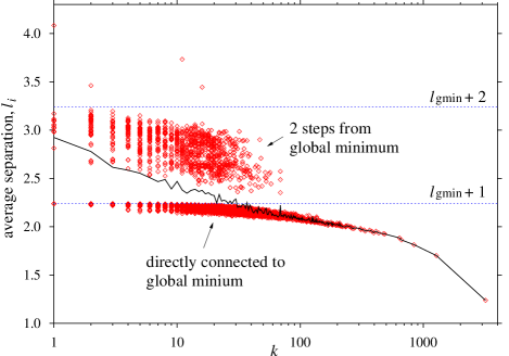
Figure 8: (Colour online). The dependence of the average separation of a node in the network from all the others on the degree. Each LJ₁₄ minimum is represented by a data point and the solid line is the average value for a given $k$. $l_{\rm gmin}$ is the average separation between the global minimum and the rest of the nodes.

In Figure 8 we show $l_{i}$, the average separation of a node $i$ from the rest of the network. It is clear that the global minimum plays a central role in the network. It is the node that is on average closest to all the other nodes in the network. Similarly, for all our networks the global minimum is one of the nodes for which all other nodes are within the radius of the network (Table 1). By contrast, low degree nodes are more on the periphery of the network. It is also apparent from Fig. 8 that the minima separate themselves into sets depending on how far they are away from the global minimum. For those that are directly connected to the global minimum, $l_{\rm gmin}+1$ is an upper bound to $l_{i}$ and $l_{i}$ would take that value if all the shortest paths involving that node passed through the global minimum. Similarly, the upper bound for those two steps away from the global minimum is $l_{\rm gmin}+2$, and so on. In fact there are only a few minima that are three steps away from the LJ₁₄ global minimum.

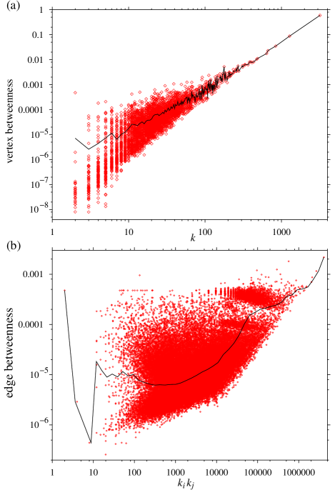
Figure 9: (Colour online). The dependence of (a) the vertex betweenness on the degree and (b) the edge betweenness on the product of degrees for LJ₁₄. Each data point represents (a) a minimum or (b) an edge, and the solid line the average value for a given (a) $k$ or (b) range of $k_{i}k_{j}$.

The vertex betweenness measures the fraction of the shortest paths between all nodes in the network that pass through a particular vertex. Similarly the edge betweenness measures the fraction of these paths that pass along a particular edge in the network. These quantities provide a measure of the importance of a node or edge to a network, particularly for dynamical processes that occur on the network, such as the passage of information. For scale-free networks, there is typically a strong correlation between the vertex betweenness and the degree,Holme et al. (2002) and Figure 9(a) shows that the inherent structure networks show a similar behaviour. The vertex betweenness has roughly a power-law dependence on $k$, and so given the scale-free degree distribution, this also implies that the probability distribution for the betweenness also has a power-law tail.Goh et al. (2002) Again the global minimum plays a central role in the network. For LJ₁₄ 59.8% of the shortest paths pass through this node.

For scale-free networks, there is also usually a correlation between the edge-betweenness and some measure of the degrees at either end of the edge, but it is much weaker than for the vertex betweenness.Holme et al. (2002) In Figure 9(b) we see such a correlation with the product of the degrees at either end of the edges for the LJ₁₄ network. However, the correlation is fairly weak and there is much more scatter in the data. The edge with maximum betweenness connects the two highest-degree nodes and 0.22% of the shortest paths pass along it.

III.5 Network Correlations

To further understand the structure of our networks, it is important to go beyond just local properties of a node to study the correlations between the properties of the nodes. Indeed correlations can have an important influence on other network properties,Dorogovtsev (2004) and have a strong effect on dynamical processes that occur on a network.Eguíluz and Klemm (2002); Boguñá et al. (2003); Vázquez and Weigt (2003); Vázquez and Moreno (2003); Echenique et al. (cond-mat/0406547)

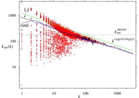
Figure 10: (Colour online). The dependence of the average degree of the neighbours of a node on the degree of that node. Each LJ₁₄ minimum is represented by a data point and the solid line labelled ‘LJ’ is the average value for a given $k$. Also included is $k_{nn}(k)$ for the randomized networks, a line with the exponent expected for an Apollonian network,Doye and Massen (cond-mat/0407779) and a line at $k_{nn}^{\rm uncorr}$, the value expected for an uncorrelated network.

Most commonly, correlations with respect to degree are investigated. For example, in Figure 10 we show how $k_{nn}$, the average degree of the neighbours a node, depends on the degree of the node. If the network were uncorrelated, one would expect $k_{nn}$ to be independent of degree and to take a value $k_{nn}^{\rm uncorr}=\langle k^{2}\rangle/\langle k\rangle$. However, $k_{nn}(k)$ has a negative slope showing that our networks are disassortative by degree, i.e. high degrees are more likely to be connected to low degree nodes than expected, and vice versa. Conversely, in assortative networks nodes are more likely to be connected to those with similar degrees. Interestingly, $k_{nn}(k)$ has an approximate power-law dependence on $k$, as seen for other scale-free networks,Pastor-Satorras et al. (2001) with an exponent that is very similar to that of an Apollonian network.Doye and Massen (cond-mat/0407779)

Another way to measure such correlations is through the assortativity coefficient introduced by Newman.Newman (2002, 2003b) It is a two-point correlation function of the properties at either end of an edge and is usually normalized by the value expected for a perfectly assortative network. It is defined as

$$r_{s}={\langle st\rangle_{e}-\langle s\rangle_{e}\langle t\rangle_{e}\over\langle st\rangle_{e,assort}-\langle s\rangle_{e}\langle t\rangle_{e}}.$$ (10)

where $s$ and $t$ correspond to the property of interest at either end of an edge, $e$ denotes that the averages are over all edges and assort that the average is for a perfectly assortative network. A positive value is expected for an assortative network (with an upper bound of 1), zero for an uncorrelated network and a negative value for a disassortative network. Negative values have been found for technological networks, such as the internet and world-wide web, and biochemical networks, such as the network of protein-protein interactions and metabolic networks, whereas strongly positive values have been found for social networks.Newman (2002, 2003b) Values of $r_{k}$ are given in Table 1 and, as with $k_{nn}(k)$ indicate the disassortative nature of our networks. The values found for the larger clusters are quite similar to those for technological networks.Newman (2002, 2003b)

The origin of this disassortativity has been explored in most depth for the internet.Pastor-Satorras et al. (2001); Maslov and Sneppen (cond-mat/0205379); Park and Newman (2003) In particular, it was found that the exclusion of multiple edges and self-connections can be a significant source of disassortativity. Indeed, when we compare $k_{nn}$ and $r_{k}$ to the values for the randomized networks (Fig. 10 and Table 2), we find very similar levels of disassortativity.

In an uncorrelated network, the probability that a randomly chosen edge will connect two particular nodes is $k_{1}k_{2}/2n_{\rm edges}^{2}$ and, hence, the total number of expected connections between the two nodes is $k_{1}k_{2}/2n_{\rm edges}$. For the LJ₁₄ network this gives an expected value of 33.5 edges between the two highest degree nodes. As only one is possible, the network appears disassortative.

Correlations also have a significant effect on the clustering.Dorogovtsev (2004); Soffer and Vázquez (cond-mat/0409686) As indicated by the expressions above, the probability that the neighbours of a node are connected depends sensitively on the degrees of the neighbours, with high degree nodes being much more likely to be connected. Hence the local clustering coefficient is higher for nodes with larger $k_{nn}$, and so even for the randomized graphs the local clustering coefficient decreases as $k$ increases (Fig. 7).

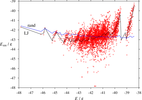
Figure 11: (Colour online). The dependence of the potential energy of the neighbours of a minima on its energy. The data points are for every LJ₁₄ minimum, and the lines binned averages for both the LJ₁₄ network, and randomized versions, as labelled.

We have also explored correlations between the potential energies of connected minima. Values of $r_{E}$ are given for both the inherent structure networks and the randomized versions in Tables 1 and 2, respectively, and the behaviour of $E_{nn}$, the average energy of the the minima to which a minimum is directly connected, is shown in Figure 11. Because of the correlations between $k$ and $E$ (Fig. 4), one might also expect the networks to be disassortative with respect to the energy of the minima. However, for $N>9$ positive values of $r_{E}$ are found, whereas the values for the randomized networks are always negative, and of roughly similar magnitude to $r_{k}^{\rm rand}$. This difference shows that the potential energy of the minima plays an important role in the structure of the network.

At low energies, $E_{nn}(E)$ has a gentle negative slope similar to that for the randomized graphs, and probably mainly reflects the exclusion of self-connections and multiple edges. The low-enegy hubs have to be connected to higher-energy minima because of the constraint that all the neighbours must be different. For example, the LJ₁₄ global minimum is connected to 3201 of the 4196 nodes. Even if these were the 3201 lowest-energy nodes (i.e. maximally assortative given the exclusion of multiple edges), the average energy of its neighbours would only be a little lower ($0.28\epsilon$) than the actual value. However, for the higher-energy nodes $E_{nn}(E)$ has a strongly positive slope, because of the preference for linking to minima with similar energy.

Although uncorrelated energy landscapes have been studied theoretically,Derrida (1980); Bryngelson and Wolynes (1987) the assumption that the energy of connected states is independent is usually unrealistic and gives rise to landscapes that are extremely rough. (Indeed the first step in incorporating greater realism in these models is often to include correlations.Saven et al. (1994); Wang et al. (1996)) For landscapes associated with the configurations of atomic systems, the landscapes are much smoother, simply because connected states are likely to be structurally similar and hence have similar energies. However, it should be remembered that the measures of correlations we have used here are quite local, and apply to just the immediate neighbourhood of a basin. When energy landscapes are inferred to be rough, e.g. because the system is a good glass-former and easily gets stuck in traps on the landscape,Stillinger (1995) this is usually referring to a lack of correlations at larger length scales.

IV Dynamical Implications

So far, we have made a detailed characterization of the network of connections between the minima on a potential energy surface, and these results provide important insights into the fundamental organization of energy landscapes. But it is also important to understand the implications of this topology for the dynamics of a system.

Clearly, the small-world nature of the inherent structure networks has important consequences for the theoretical understanding of searching configuration space. For example, the Levinthal paradox in protein folding highlights the huge number of possible configurations of a protein and the seeming impossibility of reaching the native state in a random search through these configurations, in contrast to the protein’s actual ability to fold.Lev Similar paradoxes can of course be formulated for any system with a large configuration space, be it a macromolecule, cluster or bulk liquid, that is able to routinely find a preferred structure. More formally, the exponential increase in the size of the search space underlies the classification of most problems involving the global optimization of a configuration as “NP-hard”;Garey and Johnson (1979) i.e. there is no known algorithm that is guaranteed to solve the problem in polynomial time.

Our results offer part of the answer to these paradoxes. Even for high-dimensional configuration spaces with huge numbers of accessible states, the number of steps in a pathway from a random configuration to the target state remains modest due to the favourable scaling with size (Eq. (9)). Of course, finding that particular pathway in the absence of additional guiding information can be extremely hard, although there is some evidence that a local knowledge of the topology can be of some help.Adamic et al. (2001); Kim et al. (2002) Indeed, the emphasis of most proposed solutions to the Levinthal paradox is on those features of the energy landscape, such as funnels,Leopold et al. (1992); Bryngelson et al. (1995) that guide the system in the right direction in its descent down the energy landscape, and whose presence differentiates those systems that are able to find the target state, from those that get stuck in the morass of possible configurations.

The dramatic consequences of this small-world behaviour are evidenced in examples where the energy landscape has a favourable topography. For example, for LJ₅₅ it has been estimated that there are $10^{21}$ minima. However, the basin-hopping global optimization algorithm is able to find the global minimum from a random starting point after sampling on average only approximately 150 minima.Doye et al. (1998)

The scale-free nature of the inherent structure network will also have important implications for a system’s dynamics. Interestingly, at the centre of Leopold et al’s original definition of a folding funnel was the concept of a “convergence of multiple pathways” at the native state of a protein.Leopold et al. (1992) Interpreting this idea in network terms, it seems to be suggesting that the native state would be a hub in the network. For our inherent structure networks we see such convergence with the global minimum connected to a significant fraction of the other minima, and similar results have been obtained in Rao et al.’s investigation of the connectivity of configuration space for polypeptide chains.Rao and Caflisch (2004) Of course, there is also a strong topographical component inherent in the idea of a funnel, namely that as the system goes downhill it is becoming closer to the native state, and it is this feature that has received the most emphasis more recently, perhaps to the neglect of the potential focussing aspects of the topology.

A wide variety of dynamical processes have been studied on complex networks. The dynamics of interest here is the molecular dynamics on the potential energy surface, as dictated by the forces on the system. The most relevant work to this from the networks literature is that examining diffusion on scale-free networks,Bollt and ben Avraham (cond-mat/0409465) where it was found that this topology led to more favourable scaling of the transit time between nodes, particularly when these nodes had high-degree.

The effect of the topology on the dynamics on an energy landscape can be illustrated for a simple model landscape where topographical features are eliminated. The model consists of a a flat landscape where all the minima are identical, except for their connectivity, i.e. they have the same energies and vibrational (and hence thermodynamical) properties, and furthermore, all the transition rates between connected minima take the same value $k^{\dagger}$. The average residence time in a minimum $i$ is then $1/k_{i}k^{\dagger}$. As the equilibrium probability of being in a minimum $i$ is simply $1/n_{\rm min}$, the frequency with which this minimum is visited is $k_{i}k^{\dagger}/n_{\rm min}$. The first passage time for encountering a minimum therefore decreases with degree. The topology of the inherent structure network has a focussing effect directing the system more rapidly to the highly-connected hubs. The effects of the topology on the dynamics will be explored in more detail in future work.

V Conclusion

In this paper we have provided a detailed characterization of the inherent structure networks for a series of small Lennard-Jones clusters. These networks show the mixture of local order (as measured by clustering coefficients) and small average separations between nodes that is characteristic of small-world networks.Watts and Strogatz (1998) Furthermore as the size of the clusters increase, these inherent structure networks develop a clear power-law tail to the degree distribution and have a whole variety of properties that are typical of scale-free networks.

However, in contrast to most scale-free networks the origin of this scale-free topology is not due to some form of preferential attachment during network growth.Barabási and Albert (1999) Instead, the network heterogeneity reflects the topography of the energy landscape with the degree of a node strongly correlated to the potential energy of the associated minimum. This correlation most likely arises because the low-energy minima have larger basins of attraction, and so are likely to have more transition states located on their basin boundaries. Apollonian networks provide a model of how such basins could be organized to give rise to a scale-free network. Hence, the discovery of the scale-free character of inherent structure networks may have profound implications for our understanding of the way the inherent structure mapping divides up configuration space, and raises the possibility that configuration space is tiled by a fractal, Apollonian-like packing of basins.

The results presented here for the inherent structure networks are for systems interacting with a particular potential and of small size, so it is natural to ask how general are the results. Firstly, we see no obvious reason why the Lennard-Jones potential should be “special”, producing scale-free networks, while the landscapes associated with other potentials have different topologies. However, it is conceivable that differences might arise as a result of the orientational degrees of freedom associated with molecular (not atomic) systems or the constraints of chain connectivity associated with polymers, and we intend to explore this further in future work. The work of Rao and Caflisch is also of interest in this regard, because the networks they constructed to represent the configuration space connectivity of polypeptides also showed scale-free behaviour.Rao and Caflisch (2004)

Secondly, because of the exponential increase in the number of minima and transition states with system size, the analysis we presented here is inevitably limited to relatively small sizes. Furthermore, there is currently no known method to construct a statistical representation of the inherent structure network from an incomplete sampling of the network. One potential way to analyse systems of larger size is to use a more coarse-grained division of configuration space than provided by the inherent structure mapping, such as that used by Rao and Caflisch.Rao and Caflisch (2004) Another more indirect approach would be to probe properties that sensitively reflect the underlying network topology. For example, the analogy to Apollonian networks suggests that the distribution of basin areas should follow a power law with an exponent approximately equal to -2.Doye and Massen (cond-mat/0407779)

References

- Wales (2003) D. J. Wales, Energy Landscapes (Cambridge University Press, Cambridge, 2003).
- Bryngelson et al. (1995) J. D. Bryngelson, J. N. Onuchic, N. D. Socci, and P. G. Wolynes, Proteins 21, 167 (1995).
- Stillinger and Weber (1984) F. H. Stillinger and T. A. Weber, Science 225, 983 (1984).
- Stillinger (1995) F. H. Stillinger, Science 267, 1935 (1995).
- Debenedetti and Stillinger (2001) P. G. Debenedetti and F. H. Stillinger, Nature 410, 259 (2001).
- (6) C. Levinthal, in Mössbauer Spectroscopy in Biological Systems, Proceedings of a Meeting Held at Allerton House, Monticello, Illinois, edited by J. T. P. DeBrunner and E. Munck (University of Illinois Press, Illinois, 1969), pp. 22–24. A copy of this difficult to locate citation classic can be found on the web at http://www-wales.ch.cam.ac.uk/mark/levinthal/levinthal.html.
- Stillinger and Weber (1982) F. H. Stillinger and T. A. Weber, Phys. Rev. A 25, 978 (1982).
- Stillinger (1999) F. H. Stillinger, Phys. Rev. E 59, 48 (1999).
- Tsai and Jordan (1993) C. J. Tsai and K. D. Jordan, J. Phys. Chem. 97, 11227 (1993).
- Doye and Wales (2002) J. P. K. Doye and D. J. Wales, J. Chem. Phys. 116, 3777 (2002).
- Wales and Doye (2003) D. J. Wales and J. P. K. Doye, J. Chem. Phys. 119, 12409 (2003).
- Shell et al. (2004) M. S. Shell, P. G. Debenedetti, and A. Z. Panagiotopoulos, Phys. Rev. Lett. 92, 035506 (2004).
- Sciortino et al. (1999) F. Sciortino, W. Kob, and P. Tartaglia, Phys. Rev. Lett. 83, 3214 (1999).
- Büchner and Heuer (1999) S. Büchner and A. Heuer, Phys. Rev. E 60, 6507 (1999).
- Doye (2002) J. P. K. Doye, Phys. Rev. Lett. 88, 238701 (2002).
- Strogatz (2001) S. H. Strogatz, Nature 410, 268 (2001).
- Albert and Barabási (2002) R. Albert and A. L. Barabási, Rev. Mod. Phys. 74, 47 (2002).
- Barabási (2002) A. L. Barabási, Linked: The New Science of Networks (Perseus Publishing, Cambridge, 2002).
- Bornholdt and Schuster (2003) S. Bornholdt and H. G. Schuster, eds., Handbook of Graphs and Networks: From the Genome to the Internet (Wiley-VCH, Weinheim, 2003).
- Dorogovtsev and Mendes (2003) S. N. Dorogovtsev and J. F. F. Mendes, Evolution of Networks: From Biological Nets to the Internet and WWW (Oxford University Press, Oxford, 2003).
- Newman (2003a) M. E. J. Newman, SIAM Rev. 45, 167 (2003a).
- Watts and Strogatz (1998) D. J. Watts and S. H. Strogatz, Nature 393, 440 (1998).
- Erdős and Rényi (1959) P. Erdős and A. Rényi, Publ. Math. Debrecen 6, 290 (1959).
- Erdős and Rényi (1960) P. Erdős and A. Rényi, Magyar Tud. Akad. Mat. Kutató Int. Közl. 5, 17 (1960).
- Barabási and Albert (1999) A. L. Barabási and R. Albert, Science 286, 509 (1999).
- Hughes et al. (2003) D. Hughes, M. Paczuski, R. O. Dendy, P. Helander, and K. G. McClements, Phys. Rev. Lett. 90, 131101 (2003).
- Baiesi and Paczuski (2004) M. Baiesi and M. Paczuski, Phys. Rev. E 69, 066106 (2004).
- Albert et al. (1999) R. Albert, H. Jeong, and A. L. Barabási, Nature 401, 130 (1999).
- Jeong et al. (2000) H. Jeong, B. Tombor, R. Albert, Z. N. Oltvai, and A. L. Barabási, Nature 407, 651 (2000).
- Jeong et al. (2001) H. Jeong, S. Mason, A. L. Barabási, and Z. N. Oltvai, Nature 411, 41 (2001).
- Dunne et al. (2002) J. A. Dunne, R. J. Williams, and N. D. Martinez, Proc. Natl. Acad. Sci. USA 99, 12917 (2002).
- Liljeros et al. (2001) F. Liljeros, C. R. Edling, L. A. N. Amaral, H. E. Stanley, and Y. Aberg, Nature 411, 907 (2001).
- (33) The temperature at which this time scale separation disappears was labelled by GoldsteinGoldstein (1969) and has been found to be near to the mode-coupling temperature.Schrøder et al. (2000)
- Taketsugu and Wales (2002) T. Taketsugu and D. J. Wales, Mol. Phys. 100, 2793 (2002).
- Newman (2002) M. E. J. Newman, Phys. Rev. Lett. 89, 208701 (2002).
- Newman (2003b) M. E. J. Newman, Phys. Rev. E 67, 026126 (2003b).
- Miller et al. (1999) M. A. Miller, J. P. K. Doye, and D. J. Wales, Phys. Rev. E 60, 3701 (1999).
- Doye and Wales (1999) J. P. K. Doye and D. J. Wales, Phys. Rev. B 59, 2292 (1999).
- Wales (2002) D. J. Wales, Mol. Phys. 100, 3285 (2002).
- Berry and Breitengraser-Kunz (1995) R. S. Berry and R. Breitengraser-Kunz, Phys. Rev. Lett. 74, 3951 (1995).
- Amaral et al. (2000) L. A. N. Amaral, A. Scala, M. Barthélémy, and H. E. Stanley, Proc. Nat. Acad. Sci. USA 97, 11149 (2000).
- Scala et al. (2001) A. Scala, L. A. Nunes Amaral, and M. Barthélémy, Europhys. Lett. 55, 594 (2001).
- Wuchty (2003) S. Wuchty, Nucleic Acids Res. 31, 1108 (2003).
- Rao and Caflisch (2004) F. Rao and A. Caflisch, J. Mol. Biol. 342, 299 (2004).
- (45) See http://www-doye.ch.cam.ac.uk/networks/LJn.html.
- Jortner (1992) J. Jortner, Z. Phys. D 24, 247 (1992).
- (47) In Ref. Doye, 2002 we gave the result . The error in our calculation was to exclude terms with in Eq. 6, before multiplying by . However, the result of this is to exclude from the average all paths between nodes that have the same value for one of the lattice coordinates, rather than just between a node and itself, as we had intended. This mistake did not affect the main point of the calculation, the logarithmic scaling of with the number of lattice points, but just the prefactor to Eq. 7.
- (48) As noted by Tsallis and co-workersTsallis (2004); Soares et al. (cond-mat/0410459) the cumulative degree distribution can in fact be well fitted to a function of the form , where the exponential is defined as ; note that .
- Cohen and Havlin (2003) R. Cohen and S. Havlin, Phys. Rev. Lett. 90, 058701 (2003).
- Chung and Lu (2002) F. Chung and L. Lu, Proc. Natl. Acad. Sci. USA. 99, 15879 (2002).
- Caldarelli et al. (2002) G. Caldarelli, A. Capocci, P. De Los Rios, and M. A. Muñoz, Phys. Rev. Lett. 89, 258702 (2002).
- Heuer and Büchner (2000) A. Heuer and S. Büchner, J. Phys.-Condens. Mat. 12, 6535 (2000).
- Doye et al. (1998) J. P. K. Doye, D. J. Wales, and M. A. Miller, J. Chem. Phys. 109, 8143 (1998).
- Stillinger and Stillinger (1990) F. H. Stillinger and D. K. Stillinger, J. Chem. Phys. 93, 6106 (1990).
- Bytheway and Kepert (1992) I. Bytheway and D. L. Kepert, J. Math. Chem. 9, 161 (1992).
- Mandelbrot (1983) B. B. Mandelbrot, The Fractal Geometry of Nature (W. H. Freeman, New York, 1983).
- Manna and Herrmann (1991) S. S. Manna and H. J. Herrmann, J. Phys. A 24, L481 (1991).
- Doye and Massen (cond-mat/0407779) J. P. K. Doye and C. P. Massen (cond-mat/0407779).
- Andrade et al. (cond-mat/0406295) J. S. Andrade, H. J. Herrmann, R. F. S. Andrade, and L. R. da Silva (cond-mat/0406295).
- Maslov and Sneppen (2002) S. Maslov and K. Sneppen, Science 296, 910 (2002).
- Milo et al. (cond-mat/0312028) R. Milo, N. Kashtan, S. Itzkovitz, M. E. J. Newman, and U. Alon, Phys. Rev. E p. in press (cond-mat/0312028).
- Ravasz et al. (2002) A. L. Ravasz, E. Somera, D. A. Mongru, Z. N. Oltvai, and A. L. Barabási, Science 297, 1551 (2002).
- Ravasz and Barabási (2003) E. Ravasz and A. L. Barabási, Phys. Rev. E 67, 026112 (2003).
- Serrano and Boguñá (2003) M. A. Serrano and M. Boguñá, Phys. Rev. E 68, 015101(R) (2003).
- Cancho et al. (2004) R. F. i. Cancho, , R. V. Solé, and R. Köhler, Phys. Rev. E 69, 051915 (2004).
- Vázquez et al. (2003) A. Vázquez, R. Pastor-Satorras, and A. Vespignani, Phys. Rev. E 65, 066130 (2003).
- Dorogovtsev et al. (2002) S. N. Dorogovtsev, A. V. Goltsev, and J. F. F. Mendes, Phys. Rev. E 65, 066122 (2002).
- Comellas et al. (2004) F. Comellas, G. Fertin, and A. Raspaud, Phys. Rev. E 69, 037104 (2004).
- Dorogovtsev (2004) S. N. Dorogovtsev, Phys. Rev. E 69, 027104 (2004).
- Maslov and Sneppen (cond-mat/0205379) S. Maslov and K. Sneppen (cond-mat/0205379).
- Park and Newman (2003) J. Park and M. E. J. Newman, Phys. Rev. E 68, 026112 (2003).
- Holme et al. (2002) P. Holme, B. J. Kim, C. N. Yoon, and S. K. Han, Phys. Rev. E 65, 056109 (2002).
- Goh et al. (2002) K.-I. Goh, E. Oh, H. Jeong, B. Kahng, and D. Kim, Proc. Natl. Acad. Sci. USA 99, 12583 (2002).
- Eguíluz and Klemm (2002) V. M. Eguíluz and K. Klemm, Phys. Rev. Lett. 89, 108701 (2002).
- Boguñá et al. (2003) M. Boguñá, R. Pastor-Satorras, and A. Vespignani, Phys. Rev. Lett. 90, 028701 (2003).
- Vázquez and Weigt (2003) A. Vázquez and M. Weigt, Phys. Rev. E 67, 027101 (2003).
- Vázquez and Moreno (2003) A. Vázquez and Y. Moreno, Phys. Rev. E 67, 015101(R) (2003).
- Echenique et al. (cond-mat/0406547) P. Echenique, J. Gómez-Gardenes, Y. Moreno, and A. Vázquez (cond-mat/0406547).
- Pastor-Satorras et al. (2001) R. Pastor-Satorras, A. Vásquez, and A. Vespignani, Phys. Rev. Lett. 87, 258701 (2001).
- Soffer and Vázquez (cond-mat/0409686) S. N. Soffer and A. Vázquez (cond-mat/0409686).
- Derrida (1980) B. Derrida, Phys. Rev. Lett. 45, 79 (1980).
- Bryngelson and Wolynes (1987) J. D. Bryngelson and P. G. Wolynes, Proc. Natl. Acad. Sci. USA 84, 7524 (1987).
- Saven et al. (1994) J. G. Saven, J. Wang, and P. G. Wolynes, J. Chem. Phys. 101, 11037 (1994).
- Wang et al. (1996) J. Wang, J. G. Saven, and P. G. Wolynes, J. Chem. Phys. 105, 11276 (1996).
- Garey and Johnson (1979) M. R. Garey and D. S. Johnson, Computers and Intractability: A Guide to the Theory of NP-Completeness (WH Freeman, San Francisco, 1979).
- Adamic et al. (2001) L. A. Adamic, R. M. Lukose, A. R. Puniyani, and B. A. Huberman, Phys. Rev. E 64, 046135 (2001).
- Kim et al. (2002) B. J. Kim, C. N. Yoon, S. K. Han, and H. Jeong, Phys. Rev. E 65, 027103 (2002).
- Leopold et al. (1992) P. E. Leopold, M. Montal, and J. N. Onuchic, Proc. Natl. Acad. Sci. USA 89, 8721 (1992).
- Bollt and ben Avraham (cond-mat/0409465) E. M. Bollt and D. ben Avraham (cond-mat/0409465).
- Goldstein (1969) M. Goldstein, J. Chem. Phys. 51, 3728 (1969).
- Schrøder et al. (2000) T. B. Schrøder, S. Sastry, J. C. Dyre, and S. C. Glotzer, J. Chem. Phys. 112, 9834 (2000).
- Tsallis (2004) C. Tsallis, Phys. Rev. E 69, 038101 (2004).
- Soares et al. (cond-mat/0410459) D. J. B. Soares, C. Tsallis, A. M. Mariz, and L. R. da Silva (cond-mat/0410459).