Localised magnetic excitations of coupled impurities in a transverse Ising ferromagnet

Abstract

A Green’s function formalism is used to calculate the spectrum of excitations of two neighboring impurities implanted in a semi-infinite ferromagnetic. The equations of motion for the Green’s functions are determined in the framework of the Ising model in a transverse field and results are given for the effect of the exchange coupling, position and orientation of the impurities on the spectra of localized spin wave modes.

1 Introduction

Solids are known to support a variety of elementary excitations, such as phonons, polaritons and magnons. In order to model the behavior of these excitations, one often makes the assumption that the media in which they propagate can be treated as a perfect crystal with infinite extension. This approximation, however, does not alway give a reliable picture of the system. An example is given by low-dimension media, such as ultra-thin films, in which the presence of surfaces has been shown to strongly influence their spectra of excitations. That is also true for media containing impurities or defects. These different behaviors occur due to the fact that the presence of interfaces or defects in an otherwise ideal medium can modify the microscopic interactions in the material. Also, the low dimensionality of the medium, together with the presence of impurities, acts to break the translational symmetry of the system, causing significant modifications on the propagation of the excitations, and also allowing the existence of localized excitation modes.

In the case of magnetic materials, the properties of localized excitations such as surface and impurity modes have been widely studied, theoretically as well as experimentally [1, 2, 3, 4] and several models have been proposed to elucidate the dynamics of these modes. Among these, the transverse Ising model, in particular, has been shown to give a good theoretical description of real materials with anisotropic exchange (e.g., CoCs₃Cl₅ and DyPO₄) and of materials in which the crystal field ground state is a singlet [5].

The Ising model in a transverse field has been applied to ferromagnets to obtain the spin wave (SW) spectrum of semi-infinite media [6, 7] and films [8, 9, 10]. The SW frequencies associated with the presence of a impurity layer in an otherwise uniform semi-infinite medium has also attracted attention. In both cases the impurities, while breaking the translational symmetry along the direction perpendicular to the surface of the media, were assumed to be uniformly distributed along the plane of the film layers. The results showed the presence of localized impurity modes which were found to depend on the position of the impurity layer within the film, as well as on the strength of the exchange coupling between the magnetic impurity sites. A different aspect of this problem is to consider the effect of the presence of localized impurities in the medium. In the present paper we make an extension of the theory presented in Ref.[11], by considering the effect of several localized impurities in an otherwise pure semi-infinite ferromagnet, in the context of the transverse Ising model. Numerical results are obtained by means of a Green’s function technique. The paper is structured as follows: in section II the theoretical method is introduced. Numerical results are presented and discussed in section III. In section IV the main results are summarized and conclusions are presented.

2 Model and Green’s function formalism

We consider a semi-infinite ferromagnet with a (001) surface and a simple cubic structure (lattice constant $a$). Two nearest- neighbor localized impurities spins are taken to be embedded in the medium at distance $(n-1)a$ from the surface (where integer $n\geq 1$). The localized spins are described by the transverse Ising model and the Hamiltonian of the system in the presence of an external field can be written as

$${\mathcal{H}}=-\frac{1}{2}\sum_{l,m}J_{lm}S_{l}^{z}S_{m}^{z}-\sum_{l}h_{l}S_{l}^{x}$$ (1)

where $S_{l,m}^{x}$ and $S_{l,m}^{z}$ are the $x$ and $z$ components of the spin operator ${\mathbf{S}}$, with $S=\frac{1}{2}$ for all sites. The first term in the right hand side of Eq. (1) contains the contribution due to the exchange interaction. Throughout this paper we assume that the summation runs over nearest neighbor sites. The second term on the right hand side of Eq. (1) refers to the effect of the transverse magnetic field in a given site $l$ (this field is $h$ for host sites in the bulk and $h_{S}$ for host sites at the surface). For convenience, we shall re-express the Hamiltonian as ${\mathcal{H}}={\mathcal{H}}_{0}+{\mathcal{H}}_{I}$, where ${\mathcal{H}}_{0}$ is the Hamiltonian of a pure host ferromagnet, whereas ${\mathcal{H}}_{I}$ corresponds to the perturbation caused by impurities.

$${\mathcal{H}}_{I}={\mathcal{H}}_{od}+{\mathcal{H}}_{o^{\prime}d^{\prime}}+{\mathcal{H}}_{oo^{\prime}}$$ (2)

where the ${\mathcal{H}}_{od}$ (${\mathcal{H}}_{o^{\prime}d^{\prime}}$) terms contain the exchange coupling between an impurity at a given site labeled $o$ ($o^{\prime}$) and its neighboring host sites. These terms can be written as

$${\mathcal{H}}_{od}=-(J_{o}-J)\sum_{d}S_{d}^{z}S_{o}^{z}-(h_{o}-h)S_{o}^{x},$$ (3)

$${\mathcal{H}}_{o^{\prime}d^{\prime}}=-(J_{o^{\prime}}-J)\sum_{d^{\prime}}S_{d^{\prime}}^{z}S_{o^{\prime}}^{z}-(h_{o^{\prime}}-h)S_{o^{\prime}}^{x},$$ (4)

$${\mathcal{H}}_{oo^{\prime}}=-(J_{I}-J)S_{o}^{z}S_{o^{\prime}}^{z}.$$ (5)

where the $d$ ($d^{\prime}$) index labels the nearest neighbor host sites. The exchange constant assumes the values $J_{o}=J^{\prime}$ ($J_{o^{\prime}}=J^{\prime\prime}$) for the interaction between the impurities and host sites in the interior of the medium and $J_{o}=J_{S}^{\prime}$ ($J_{o^{\prime}}=J_{S}^{\prime\prime}$) when both sites are at the surface and $J$ otherwise. Likewise, the term ${\mathcal{H}}_{oo^{\prime}}$ in the Eq.(2) expresses the exchange interaction between the impurities. The Zeeman contribution in Eqs.(3) and (4) describes the effect of the transverse magnetic field at the impurities, $h_{o}$ and $h_{o^{\prime}}$, which assume the values $h^{\prime}_{S}$ and $h^{\prime\prime}_{S}$ if those are located at the surface of the medium, and $h^{\prime}$ and $h^{\prime\prime}$ otherwise.

Figure 1: Representation of the interaction scheme for two nearest neighbor impurities in a Ising ferromagnet in a transverse field. The impurities (black circles) are exchange coupled with each other and with their nearest neighbors in the host medium, and may be aligned along (a) the $x$ axis or (b) the $z$ axis.

Since we are considering only nearest neighbor spin interactions, we can distinguish two physically distinct orientations for the impurities, namely: one with the two impurities aligned along the $x$ axis, which we will refer to as the $X$ case (Fig. 1a) and another, $Z$ case (Fig. 1b) with two impurities aligned along the $z$ axis. In order to obtain the excitation spectra of these systems, we extend the formalism for a single localized impurity presented in Ref.[11]. Thus, we start by defining the Green’s functions $\langle\langle S_{l}^{\alpha};S_{m}^{\beta}\rangle\rangle_{\omega}$, where $\alpha$ and $\beta$ stand for the Cartesian components of the spin operators and $\omega$ is a frequency label. In the present paper, we use the retarded commutator Green’s function $G_{lm}({\mathbf{q}}_{\parallel},\omega)=\left\langle\left\langle S_{l}^{z};S_{m}^{z}\right\rangle\right\rangle_{\omega}$. These functions must satisfy the equation of motion [12]

$$\begin{split}\omega\left\langle\left\langle S_{l}^{z};S_{m}^{z}\right\rangle\right\rangle_{\omega}=&\frac{1}{2\pi}\left\langle\left[S_{l}^{z},S_{m}^{z}\right]\right\rangle\qquad\qquad\\ &\quad+\left\langle\left\langle\left[S_{l}^{z},{\mathcal{H}}\right];S_{m}^{z}\right\rangle\right\rangle_{\omega}.\end{split}$$ (6)

Previous calculations for the pure system showed that a second order phase transition should occur at a temperature $T_{C}$, with $\tanh{(h/2k_{B}T_{C})}=h/3J$, where $k_{B}$ denotes Boltzmann’s constant, such that for $T<T_{C}$ the average spin orientation at each site can have components in the $x$ and $y$ directions, whereas for $T>T_{C}$ it lies along the $x$ direction. The presence of impurities in the system is expected to change the critical temperature to $T_{C}^{i}$, which in some cases may be greater than $T_{C}$. In order to simplify the calculations, in this work we focus on the high-temperature regime (i.e. $T>T_{C}^{i}$). The Green’s function for the pure system can be obtained by solving Eq. (6) with ${\mathcal{H}}$ replaced by ${\mathcal{H}}_{0}$. The solution, which describes an ideal semi-infinite Ising ferromagnet (i.e., with translational symmetry parallel to the surface), is well known and is given by [13]

$$G^{0}_{lm}(\omega)=-\frac{1}{M}\sum_{q}G^{0}_{{\mathbf{q}}_{\parallel}}(\omega)\exp{[{\mathbf{q}}_{\parallel}\cdot({\mathbf{r}}_{l}-{\mathbf{r}}_{m})]},$$ (7)

where the vectors ${\mathbf{r}}_{l}$ and ${\mathbf{r}}_{m}$ indicate the positions of two given sites $l$ and $m$, ${\mathbf{q}}_{\parallel}\equiv(q_{x},q_{y})$ is an in-plane wave vector and $M$ is the number of sites in any layer parallel to the surface. The Fourier amplitudes of this function are found as

$$\begin{split}G^{0}_{{\mathbf{q}}_{\parallel}}(\omega)=&\frac{1}{2\pi J(x-x^{-1})}\\ &\times\left(x^{|n-n^{\prime}|}-\frac{1+x^{-1}\Delta}{1+x\Delta}x^{n+n^{\prime}}\right).\end{split}$$ (8)

Here the labels $n$ and $n^{\prime}$ are layer indices for the sites $l$ and $m$, respectively (with $n=1$ being the surface layer.), and $x$ is a complex number that satisfies the condition

$$x+x^{-1}=[h^{2}-4hJR^{x}\gamma({\mathbf{q}}_{\parallel})-\omega^{2}]/hJR^{x}$$ (9)

where $\gamma({\mathbf{q}}_{\parallel})$ is a structure factor that, in the case of a simple cubic lattice, is given by $\gamma({\mathbf{q}}_{\parallel})=\frac{1}{2}[\cos(q_{x}a)+\cos(q_{y}a)]$. In addition, when describing localized modes the condition $|x|\leq 1$ must also be fulfilled. The parameter $\Delta$ in Eq. (8) contains the information regarding the surface and is given by

$$\begin{split}\Delta=&\frac{\omega^{2}(h_{S}R^{x}_{S}-hR^{x})-hh_{S}(hR^{x}_{S}-h_{S}R^{x})}{hh_{S}R^{x}R^{x}_{S}J}\\ &-4\gamma({\mathbf{q}}_{\parallel})\left(\frac{J_{S}}{J}-1\right),\end{split}$$ (10)

where, from mean field theory, we obtain the spin averages at the bulk and surface as $R^{x}\equiv\langle S^{x}\rangle=\tanh{(h/2k_{B}T)}$ and $R_{S}^{x}=\tanh{(h_{S}/2k_{B}T)}$, respectively.

The presence of localized impurities in an otherwise ideal medium acts to break the translational invariance of the system. Consequently, the calculations for the impure system must be performed in real space. By including the effects of the impurity in the Hamiltonian and applying Eq. (8), one can obtain a new Green’s function $G_{lm}(\omega)$, which is found to obey the equations

$$\begin{split}A_{lj}G_{lm}(\omega)=&\quad\delta_{lj}-\\ &\frac{2\pi}{R^{x}_{l}}[P_{lj}-U_{lj}-U^{\prime}_{lj}-U^{\prime\prime}_{lj}]G_{lm}(\omega)\end{split}$$ (11)

where

$$A_{lj}=\frac{\omega^{2}-[h+(h_{o}-h)\delta_{lo}+(h_{o^{\prime}}-h)\delta_{lo^{\prime}}]^{2}}{h+[h+(h_{o}-h)\delta_{lo}+(h_{o^{\prime}}-h)\delta_{lo^{\prime}}]}\delta_{lj},$$

$$P_{lj}=\sum_{p}J_{lp}R_{l}^{x}\delta_{lj}$$

$$U_{lj}=\sum_{d}(J_{o}-J)\,R_{l}^{x}[\delta_{lo}\delta_{dm}+\delta_{ld}\delta_{jo}],$$

$$U^{\prime}_{lj}=\sum_{d^{\prime}}(J_{o^{\prime}}-J)\,R_{l}^{x}[\delta_{lo^{\prime}}\delta_{jd^{\prime}}+\delta_{ld^{\prime}}\delta_{jo^{\prime}}],$$

$$U^{\prime\prime}_{lj}=(J_{I}-J)\,R_{l}^{x}[\delta_{lo^{\prime}}\delta_{jo}+\delta_{lo}\delta_{jo^{\prime}}].$$

where the index $o$ ($o^{\prime}$) assumes the values $0$ ($2$) for each impurity site in the $X$ case and $0$ ($6$) in the $Z$ case (see Fig. 1). The second summation runs over $5$ neighboring host sites to either impurity. By rewriting Eq. (11) in matrix form we obtain the Dyson equation

$$[({\mathbf{\tilde{G}}}^{0}(\omega))^{-1}-{\mathbf{V}}]{\mathbf{\tilde{G}}(\omega)}={\mathbf{I}},$$ (12)

where ${\mathbf{\tilde{G}}}^{0}(\omega)$ and ${\mathbf{\tilde{G}}}(\omega)$ are square matrices with elements given by $(2\pi/R_{l}^{x})G^{0}_{lm}(\omega)$ and $(2\pi/R_{l}^{x})G_{lm}(\omega)$, respectively. ${\mathbf{I}}$ is the unit matrix, ${\mathbf{V}}$ is an effective potential related to the impurity term ${\mathcal{H}}_{I}$, with elements

$$\begin{split}V_{lj}=&\frac{\omega^{2}-h^{2}}{h}\delta_{lj}-A_{lj}-P_{lj}\\ &-U_{lj}-U^{\prime}_{lj}-U^{\prime\prime}_{lj}.\end{split}$$ (13)

Thus, Eq. (9) can be said to relate the matrix Green’s function of the pure (${\mathbf{G}^{0}}(\omega)$) and impure (${\mathbf{G}}(\omega)$) systems. The spectrum of localized modes is then found by numerically calculating the frequencies that satisfy the determinantal condition

$$\det[\mathbf{I}-\mathbf{\tilde{G}}^{0}(\omega)\mathbf{V}]=0$$ (14)

which gives the poles of the Green’s function for the impure system.

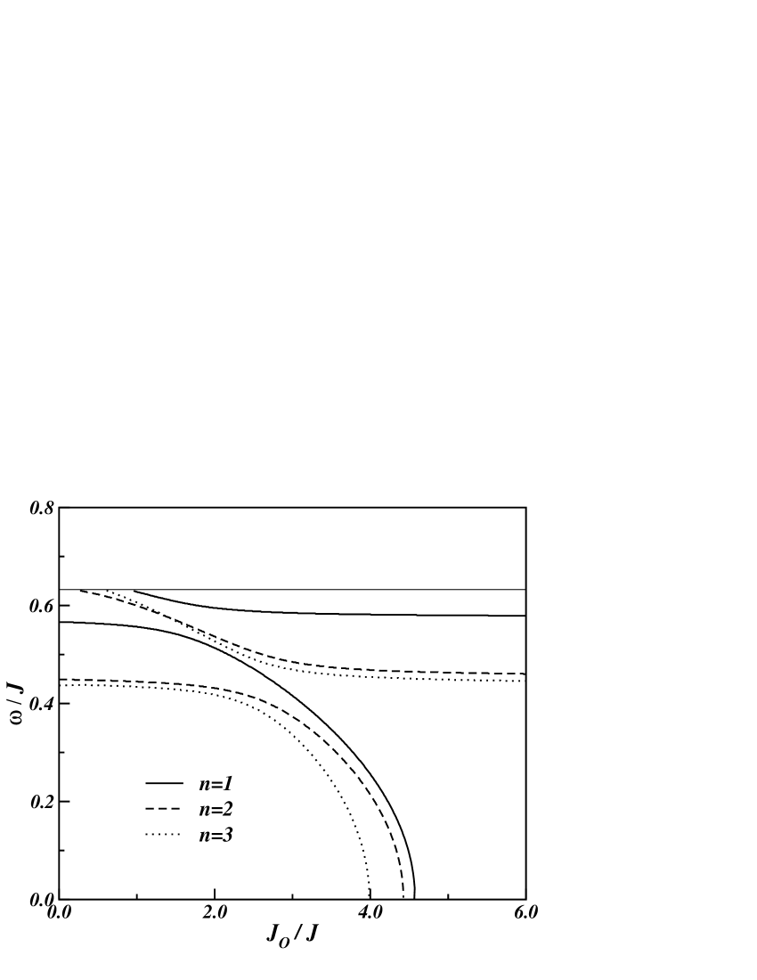
Figure 2: Localized spin wave frequencies as a function of the exchange parameter $J_{o}$, for the $X$ case, with $h_{o}=h_{o^{\prime}}=0.65h$ and $T=2.5J/k_{B}$. The parameters are $J_{o^{\prime}}=1.5J$ and $J_{I}=0.25J$ when both impurities are at the surface (solid lines), and $J_{o^{\prime}}=2.5J$, $J_{I}=0.25J$ when the two impurities are at the second(dashed lines) and third layers(dotted lines).

3 Numerical Results

Impurities modes spectra were calculated as functions of the exchange and effective field parameters. In order to assess the influence of the position of each impurity on the excitation spectra, we obtained numerical solutions of Eq.(14) for impurities located at the surface of the medium (layer 1) as well as deeper in the system (layers 2 and 3). Specifically, for the $X$ case, we considered three configurations, namely, we set $n=1$ (both impurities at the surface), $n=2$ (both impurities at the second layer) and $n=3$ (both impurities at the third layer) according to the notation in Fig. 1a. Likewise, for the $Z$ case, following Fig. 1b we set $n=1$ (i.e. one of the impurities at the surface, the other at layer 2), $n=2$ (one at layer 2, the other at layer 3) and $n=3$ (impurities at layers 3 and 4).

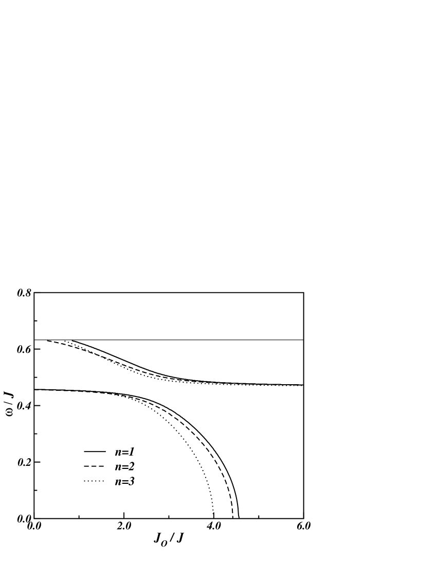
Figure 3: Localized spin wave frequencies as a function of the exchange parameter $J_{o}$ in the upper impurity in an Ising ferromagnet in a transverse field, for the $Z$ case, with $h_{o}=h_{o^{\prime}}=0.65h$ and $T=2.5J/k_{B}$. The parameters are $J_{o^{\prime}}=1.5J$ and $J_{I}=0.25J$ when the upper impurity is located at the surface (solid lines), and $J_{o^{\prime}}=2.5J$, $J_{I}=0.25J$ when the upper impurity is at the second (dashed lines) and third layers (dotted lines).

Figure 2 shows the local SW impurities spectra for the $X$ case, as a function of the exchange constant for the coupling between one of the impurities and its neighboring host sites ($J_{o}$), while the parameters for the second impurity are kept constant. We have used $J_{o^{\prime}}=1.5J$ and $J_{I}=0.25J$ for $n=1$, and $J_{o^{\prime}}=2.5J$, $J_{I}=0.25J$ for $n=2$ and $3$. The field parameters were $h_{o}=h_{o^{\prime}}=0.65h$ and we used $T=2.5J/k_{B}$ in all cases. The three sets of branches correspond to the impurities located in layers 1 (solid line), 2 (dashed line) and 3 (dotted line). The impurities modes can be classified as resonance modes (i.e. those occurring in the SW bulk band) and defect modes (those found outside the bulk band). In this work we consider defect modes, since these are easier to measure. Therefore we restrict the calculation to the region outside the bulk SW band.

The lower limit of the bulk band is represented in the graph by the horizontal line. In the absence of the coupling between the impurities, the graph would show a horizontal line (for the impurity with $J^{\prime}$ constant) superimposed on the decaying curve of the SW branch associated with the second impurity, which merges with the bulk band for low values of $J_{o}$. The exchange coupling thus creates a mode repulsion effect when $J_{o}\approx J_{o^{\prime}}$. As expected, the magnitude of this effect depends on the strength of the exchange coupling between the impurities. When both impurities are at the surface, the lower coordination number causes a large frequency shift in comparison with the other configurations.

Figure 4: Localized spin wave frequencies as a function of the exchange parameter $J_{o^{\prime}}$ in the lower impurity in an Ising ferromagnet in a transverse field, for the $Z$ case, with $h_{o}=h_{o^{\prime}}=0.65h$ and $T=2.5J/k_{B}$. The parameters are $J_{o}=1.5J$ and $J_{I}=0.25J$ when the upper impurity is located at the surface (solid lines), and $J_{o}=2.5J$, $J_{I}=0.25J$ when the upper impurity is at the second (dashed lines) and third layers (dotted lines).

The effect of the alignment of the impurities is shown in Fig. 3, which presents results for the SW frequencies in the $Z$ case, as a function of the exchange constant at the upper impurity, while the remaining parameters were kept constant. For $n=2$ and $n=3$, the results are similar to the ones obtained for $X$ case, apart from a small frequency shift. For $n=1$, however, the branches are strongly shifted. These results demonstrate that the influence of orientation becomes particularly important for impurities close to the surface. This is a consequence of the smaller number of neighbors, together with modified exchange parameters at the surface.

Figure 4 shows results of frequency as a function of $J_{o^{\prime}}$ at the lower impurity in the $Z$ case, with the remaining parameters kept constant. In this case, the exchange parameter being varied is associated with the lower impurity (see Fig. 1), which was assumed to be located at the second, third and fourth layers. In contrast with the results of Fig. 3, the frequency branches are not found to merge with the bulk band for low values of the exchange parameter. Moreover, when the lower impurity is localized at the second layer(solid line), the curves show a larger shift in comparison with the remaining configurations. This effect is a consequence of the modification of the exchange parameters for the upper impurity when located at the surface.

Figure 5: Localized spin wave frequencies as a function of the local field parameter $h_{o}$ in one of the impurities, in an Ising ferromagnet in a transverse field, for the $X$ case. The remaining parameters are the same as in the previous graphs. The results were obtained for both impurities at the first (solid lines), second (dashed lines) and third layers (dotted lines).

The influence of the local fields is shown next. Figure 5 shows the local SW frequencies as a function of local field parameter $h_{o}$ at one of the impurities, for the $X$ case. The remaining parameters are the same as in the previous graphs. The results were obtained for $n=1$ (solid lines), $n=2$ (dashed lines) and $n=3$ (dotted lines). The graphs show the mode repulsion, due to the coupling of the impurities. Also evident is a large frequency shift for $n=1$, due to the modified exchange parameters at the surface. For fields larger than $h_{o}=0.69\,h$ ($n=1$), $h_{o}=0.99\,h$ ($n=2$) and $h_{o}=1.11\,h$ ($n=3$), the upper frequency branches are found to merge with the bulk band, thus becoming resonance modes.

A similar graph is shown in Fig. 6, this time for the $Z$ case. The results were calculated for a varying local field at the upper impurity. In contrast with the previous figure, the higher frequency branches in the graph do not display any noticeable frequency shift for low values of the local field. On the other hand, the high frequency excitations are observed to become resonance modes for values of local fields that approximately the same as in the $X$ case.

Figure 7 shows a plot of frequency as a function of the exchange coupling constant for the interaction between the impurities ($J_{I}$). The graph shows results for both the $X$ and $Z$ cases, and the results were obtained for ferromagnetic ($J_{I}>0$) as well as antiferromagnetic ($J_{I}<0$) coupling. For the $X$ case, we assumed that both impurities were located at the surface of the system, whereas in the $Z$ case we considered the upper impurity at the surface, and the lower one at the second layer. The branches behave quite distinctly in each case, with the results for the $Z$ case displaying a large shift in comparison with the other case. Also prominent in the $X$ case is a mode crossing that is found for $J_{I}=-0.86J$. In contrast, the results for the $Z$ case show no mode crossings, although the low frequency is observed to have a maximum at $J_{I}=-1.11J$ and the high frequency branch has a minimum at $J_{I}=-1.37J$.

Figure 6: Localized spin wave frequencies as a function of the local field parameter $h_{o}$ for the upper impurity, in an Ising ferromagnet in a transverse field, for the $Z$ case, when the upper impurity is located at the first (solid lines), second (dashed lines) and third layers (dotted lines).

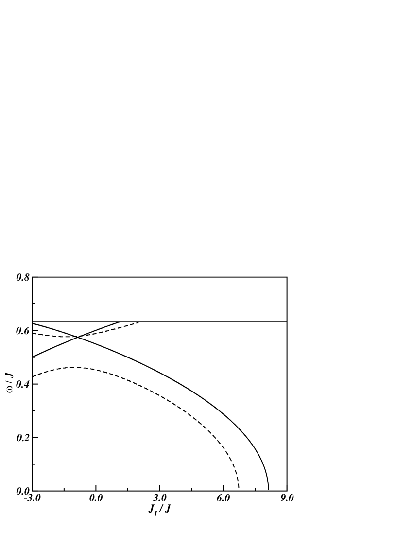
Figure 7: Localized spin wave frequencies as a function of the exchange parameter $J_{I}$ for the coupling between the impurities. The graph shows results for both the $X$ case (solid line) where the impurities are located at the surface layer, and the $Z$ case (dashed line) where one impurity is located at the surface and the other in the layer below. The remaining parameters are the same as in the previous figures.

4 Conclusions

We have presented a Green’s functions calculation of the SW frequencies of localized modes associated with two coupled localized impurities implanted in an otherwise ideal ferromagnet. The results were obtained in the context of the Ising Model in a transverse field and show the influence of the exchange coupling of the impurities on the excitation spectra of the system. This coupling modifies the spectra in relation to the results for single impurities, especially when the coupling parameters for the interactions between the impurities and the host sites are of the same magnitude. The results also point to a strong effect of the orientation of the impurities on the localized SW frequencies, especially when the impurities are located close or at the surface. Further studies could investigate the effect of the presence of the impurities on thin ferromagnetic films, as well as the effect of their coupling and orientation on the critical properties of the system as well as on the overall magnetization of the material.

The authors would like to acknowledge the financial support of the Brazilian agency CNPq.

References

- [1] M. G. Cottam and D. R. Tilley, Introduction to Surface and Superlattice Excitations, Cambridge University Press, Cambridge (1989).
- [2] Niu-Niu Chen, M. G. Cottam, Phys. Rev. B44(1991) 7466.
- [3] Niu-Niu Chen, M. G. Cottam, Phys. Rev. B45(1992) 266.
- [4] M. Henkel, Conformal Invariance and Critical Phenomena (Springer, Heidelberg, 1999).
- [5] Y. L. Wong, B. Cooper, Phys. Rev. B172, 539 (1968).
- [6] M. G. Cottam, D. R. Tilley, and B. Zeks, J. Phys. C 17, 1793 (1984).
- [7] B. A. Shiwai, M. G. Cottam, Phys. Stat. Sol. B134, 597 (1986).
- [8] A. Salman, M. G. Cottam, Surf. Sci. Lett. 1, 23 (1994).
- [9] M. G. Cottam and D. E. Kontos, J. Phys. C13, 2945 (1980).
- [10] R. Blinc, B. Zeks, J. Phys. C17, 1973 (1984).
- [11] R. N. Costa Filho, U. M. S. Costa, M. G. Cottam, J. Mag. and Mag. Mat. 189, 234-240 (1998).
- [12] D. N. Zubarev, Soviet Phys. Uspkhi 3, 320 (1960).
- [13] M. G. Cottam, J. Phys. C9, 2121 (1976).