[
Time dependence of transmission in semiconductor superlattices
Abstract
Time delay in electron propagation through a finite periodic system such as a semiconductor superlattice is studied by direct numerical solution of the time-dependent Schrödinger equation. We compare systems with and without addition of an anti-reflection coating (ARC). With an ARC, the time delay is consistent with propagation at the Bloch velocity of the periodic system, which significantly reduces the time delay, in addition to increasing the transmissivity.
03.65.Xp, 73.63.-b, 05.60.Cg
]
I Introduction
Electron transport in a layered semiconductor superlattice (SL) [1] can in many cases be treated as a one-dimensional finite periodic system. With as few as five cells, a well-developed band structure ensues [2]. Within each allowed band, where the Bloch phase increases by , the transmission shows narrow peaks determined by , . Between these peaks the transmission touches an envelope of the minima which also has a simple description. In the forbidden bands, the Bloch phase acquires an imaginary part; as a result the transmission goes rapidly to zero. Pacher et al. [3] have used this property to design an electron band-pass filter. Further, by adding a quarter-wave cell at each end of the periodic array [4, 5], they were able to increase the average transmission within the band from about to about .
In this work we will study the time dependence of an electron wavepacket passing through a superlattice, comparing the situation with and without an anti-reflection coating (ARC). In a series of papers [6, 7, 8, 9], some of the present authors have shown how to design an ARC which gives optimal transmission within a given miniband, by adding suitably configured potential cells on each end of a periodic array. The design depends on the shape of the potential cells making up the periodic array, but not their number. An -cell ARC consists of distinct potential cells on each end [8]. In the simplest case the periodic array consists of reflection symmetric cells; the ARC can also be made reflection symmetric by using symmetric cells and reversing their order at the opposite end.
In the transfer matrix formalism, the electron wave function at fixed position is represented by two amplitudes, which can be treated as a spinor. The upper component corresponds to right-moving and the lower to left-moving waves. Passing though an arbitrary potential cell is described by the action of a transfer matrix on this spinor. For reflection symmetric cells, the transfer matrix can be represented in the Kard form [8, 9, 10], which involves just two real parameters at given energy. One of these is the Bloch phase, and the second, the impedance parameter , is approximately constant over the middle of an allowed band, but diverges at the band edges. Adopting the Kard parameterization allows one the benefit of a powerful analogy to the precession of an electron spin in a magnetic field. The magnetic field direction has polar angle , where . The angle of precession is twice the Bloch phase: . An electron moving to the right corresponds to spin-up along OZ, and left-moving waves to spin-down. Passing through identical cells therefore amounts to precession by angle ; when this is an integer multiple of , the final electron state will be the same as the initial plane wave, (except for a phase,) which gives perfect transmission.
A Bloch state is one where the wave function on either side of the potential cell differs only by the Bloch phase . This is analogous to an electron whose spin is aligned along the direction of the magnetic field. The action of an ARC can therefore be understood as taking an initial spin-up state and rotating it to lie along the field direction. That is, it converts a right-moving wave into a Bloch state of the periodic array. Passing through any number of cells only adds an overall phase , and the downstream ARC reverses the alignment back to the spin-up state when the resonant condition holds.
Without an ARC, electrons which are transmitted do so via narrow resonances as mentioned above, so one expects a significant time delay. Resonant states and their characteristic time dependence [11, 12] are key parts of nuclear physics. Perhaps the definitive discussion of the time evolution of wave packets in the vicinity of resonant states is that of Rosenfeld [13]. When the ratio of resonance width to energy is small, and the wave packet is narrow in energy compared to , there is a broad range of intermediate times over which the system exhibits exponential time dependence, and therefore significant time delay compared to free propagation. The work of More and Gerjuoy [14, 15] should also be mentioned. While the 3D system differs in important ways from 1D, the same conclusion holds. The SL is an interesting system to study precisely because placing resonances within an allowed band produces resonances with widths the order of a few meV, satisfying one of Rosenfeld’s criteria.
With an ARC, propagation via a Bloch state should be much faster. To quantify this effect we have performed numerical solutions of the time-dependent Schrödinger equation (TDSE). The subject of time delay in passing though a barrier is a controversial one (see the reviews by Hauge and Støvneng [16], Leavens and Aers [17],and de Carvalho and Nussenzveig [18] for example) but it is not our purpose to debate the merits or demerits of the various definitions that have been used (phase time, dwell time, Larmor time, etc.) This controversy continues in the context of wanting to define a single time to characterize the process. Our approach is to solve the time dependent Schrödinger equation directly. This provides a direct means of comparing the two situations (with/without an ARC), while providing much more information than a single number.

There have been several papers which discuss propagation in a superlattice without an ARC. Stamp and McIntosh [19] made a careful study of the two-barrier case, which exhibits narrow quasi-bound state (QB) resonances. Their emphasis was on the role of the width (in energy) of the incident wave packet on exciting the quasi-bound states. They expanded the initial wave packet in stationary states of the scattering problem and propagated the solution in time by quadratures. This method is feasible for square barrier/well type potentials where the solutions are analytic. Pereyra [21] used a similar approach for the superlattice problem. Bouchard and Luban [22] considered electrons trapped in an infinite SL, in presence of an external electric field. Their emphasis was on the Wannier-Stark ladder of states localized by the applied field, and on finding Bloch oscillations. Their numerical method [23, 24] is similar to ours in using the implicit method to propagate the state forward in time. However, they confined the system in a box and had to limit the total time so as to avoid reflection from the walls. In our work, transparent boundary conditions remove such restrictions. The work closest to ours is by Pacher and Gornik [4, 5], who considered the effect of an ARC on transmission through a superlattice, following Pereyra for the time evolution.
The numerical method we use was pioneered by Goldberg et al. [24], and greatly improved by Moyer [25] who implemented the Numerov algorithm for the spatial variation and added transparent boundary conditions. The time-dependence is handled by the lowest-order Crank-Nicolson (implicit) method. The wave equation was followed for typically 15 ps, on a region (the “system”) of width to m. Transparent boundary conditions were especially important in obtaining our results; they were applied at both ends of the system, so that as the wave function reaches those limits, it will proceed outwards without reflection. By integrating the outgoing flux at those boundaries, the reflection and transmission probabilities are accumulated.
The initial state is a gaussian wave packet sufficiently wide in real space to correspond to a small uncertainty in energy. For the root mean square (rms) width is nm; for it is m. The main requirement on the system width is to accommodate the initial wave packet, without overlapping the potential array. Narrower (in energy) packets would require a wider system and more computer time for the simulations.
II The calculations
A Wave packet transmission
The potential array is located on near the origin, very close to . For this work we adapted a case previously studied. It corresponds to a GaAs/AlGaAs superlattice of Pacher et al., but with five barriers rather than the six of their device. Their modelling gave the barriers a height of approximately meV, and width nm, separated by wells of width nm. For convenience we used a constant effective mass in all layers. Further, to simplify the numerical work, we replaced Pacher’s square barriers by equivalent gaussian shaped barriers.
| (1) |
The gaussian barrier has height meV and a width parameter nm. The full cell width was set at nm, only wider than the square barrier cell. These parameters were fitted to make the single-cell transfer matrices equivalent within the lowest allowed band, which runs from meV. The original and the gaussian potentials are shown in Fig. 1.
By equivalent, we mean that their scattering properties are accurately the same, across the allowed band of interest. Since the transfer matrix for a symmetric cell depends on only two Kard parameters, we need only fit these two, and the results are shown in Fig. 2. The are virtually identical for the original and the gaussian potential cell, as seen in Fig. 2(a). The third (dotted) line is the of the optimal single-cell ARC. That gaussian has height meV and width parameter nm, with a total ARC cell width of nm. Also was very close for both cells: see Fig. 2(b). (The lower line is for the ARC layer. For a single-cell ARC the prescription is at the centre of the allowed band.) Having gaussian shape cells allowed us to use the Numerov method without having to worry about points of discontinuity of the potential.
| a) |  |
|---|---|
| b) | 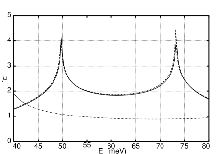 |
In Fig. 3 we show the transmission profiles of the 5-cell SL with no ARC (dotted line), a single-cell ARC (dashed line) and a two-cell ARC (solid line), for the gaussian cells array (computed using the usual time-independent methods). With the two-cell ARC, the high transmission region runs from 53 to 68 meV, and the satellite peaks are pushed closer to the band edges. This agrees well with the square barrier calculations in [6].
For solution of the time-dependent Schrödinger equation (TDSE) we chose gaussian wave packets. The initial state
| (2) |
is normalized to one particle. For a potential array sitting near the origin, the initial position has to be taken sufficiently negative so that the wave packet is well away from the periodic potential at time zero. For the more time consuming runs that followed the transmission across the entire band, a width nm was used. When producing videos of the scattering process, a less demanding nm was chosen. Most of the work was done with nm to the left of the potential array, and a gaussian wave packet centered at the mid-point of that range. For the widest wave packets employed, the amplitude of the wave at and was therefore 0.0297 for m, and was truncated to zero. The truncation introduces some high momentum components which have a small effect on time development, which is not visible in any of the graphs of this paper. Had we doubled the distances to 15 m, the truncation would have been at 8 in amplitude and not at all discernible. The fractional standard deviation in energy can be written as
| (3) |

In Fig. 4 we show transmission for the gaussian array computed using the TDSE. The right-moving flux at is
| (4) |
and the integrated transmission is
| (5) | |||||
| (6) |
The label is mean energy of the wave packet. Corresponding expressions for the reflection probability hold with the left-moving flux monitored at . For packets narrow in energy should approach the transmission probability of the time-independent solutions, and this is seen to occur. The main difference with respect to Fig. 3 is that the peaks are smeared by the finite width of the wave packet (approximately 0.5 meV). Even so, they are so narrow that the tops are ragged due to the finite steps in of the wave packets used to generate the figure. (With finer steps and narrower (in energy) wave packets, convergence has been verified.)

Also in Fig. 4, lines below the peaks show their build-up over time ; this proceeds uniformly, with some bias to faster development at higher energies. This bias can be understood as a simple velocity effect: the higher energy wave packets travel faster and reach the right wall sooner than the slower moving wave packets near the lower band edge. We note an apparent discrepancy with Fig. 4 of Romo [26]: at 0.6 ps he shows transmission in the troughs exceeding the asymptotic ( ps) transmission. However, as pointed out by an astuute reader, Romo’s calculation is based on a very different initial state than ours [27, 28]. At time his initial state is a uniform standing wave confined by a mirror to the left of the array at . The mirror is removed at , and after an infinite time a new equilibrium state is achieved which is the stationary scattering state for a wave incident from the left. As the wave front advances to the right, the leading edge becomes smeared out, and oscillations develop behind, a process which Moshinsky [27] called diffraction in time. Ultimately the limit as of should approach the time- independent transmission probability . The curves at intermediate times, at a fixed position, show the passing of the wave front and the characteristic oscillations behind it. They do not represent the accumulation of as in our calculation. Indeed, we can calculate using a long square wave packet normalized to one particle, and we find similar oscillatory behaviour in the build-up of both and the flux, which is largely absent in the time-integrated flux.
Fig. 5 shows similar results for the same array plus a single-cell ARC. Again the asymptotic transmission is in good agreement with a time-independent calculation, but smeared by the finite width of the wave packet. Also, the build-up of the transmission profile proceeds smoothly with the above-noted velocity bias.


Near each band edge there is a satellite peak which resembles the narrow resonances of the periodic array. To study the character of these lines we scanned over them using spatially narrow wave packets. We enlarged the system to the right, so that there was room for both the reflected and transmitted wave packets to become well separated from the array. We then Fourier analysed the reflected and transmitted wave packets individually. The Fourier transforms (moduli squared) and are plotted against energy in Fig. 6 and the results are quite revealing. The T packet is very narrow compared to the incident wave, and centered just below 51 meV. The R packet in contrast has a node at this energy, and corresponds to the energies on either side. This shows that the transmission does proceed primarily through a narrow resonance. The transform (mod squared) of the complete packet after scattering, denoted “sum R+T” sits right on top of the curve for the initial wave packet, which is a testament to the unitarity of the numerical work.
The time-development of the reflection and transmission probabilities is shown in Fig. 7 for a narrow (in energy) wave packet centered at meV. and (see eq. 6) are accumulated as the waves exit from the right/left boundaries . begins to rise at 2 ps; this corresponds to the time taken for part of the initial packet to be transmitted and reach . The longer time scale for is due to the wider space on the left which accommodated the initial wave packet. One sees two steps in the curve, one corresponding to direct reflection from the leading edge of the array, and the second one from entrapment before reflection. The sum is the complement of the probability remaining within the system :
| (7) |
(A 60 meV electron with effective mass travels at nm/ps; the time offsets are consistent with this.)

B Quasi-Bound states
At times near 6 ps is approaching its asymptotic value . Looking at the wave which is still trapped inside the array, one sees that it has a particular shape (shown in Fig. 8) and is decaying with mean life ps. This corresponds to a half-width meV. It implies a quasi bound state located at in the lower half complex plane. Without the ARC, the position would be slightly displaced, corresponding to the shift of the outer peaks in Fig. 3.
An electron inside the array sees four potential wells between the five stronger barriers. The QB states are built on the ground state in each well. Through coupling across the barriers four QB states are created, associated with the four transmission peaks seen in Fig. 4 for example. Fig. 8 shows that even with the ARC, the first of these states persists (as does the last). Rosenfeld [13] discussed in detail the conditions under which the exponential decay of such states would be observed; the most important is that the ratio , which is well satisfied for our superlattice. Stamp and McIntosh [19] emphasized another criterion, the “interaction time” of the wave with the potential. This is basically the dwell time inside the potential. If it is too long compared to the lifetime of the QB state, the state will be decaying continuously as it is being fed, and the probability will not be built up to a significant extent. For the state of Fig. 8, is of the same order as the time delay shown in Fig. 10, below.

The fourth QB state also survives the addition of the ARC, and implies a pole at meV. The drawing would look very similar to Fig, 8, except that the wave function has nodes in each barrier. That is because the lowest state is nodeless, while the fourth state has alternating signs in the four wells.
III Time Delay
A Results from time-dependent calculations
The primary motivation for this work was to compare the time taken to traverse the array plus ARC, as compared to the simple array. However, in the case with ARC, the two satellite peaks appear to be narrow resonances of the same type as for the simple periodic array. Hence it is also of interest to compare transmission through the satellite peaks with transmission via the Bloch states of the broad central maximum.
Fig. 7 shows that the build-up of the transmission peak at 51 meV proceeds linearly in time, over the range . Similar linear behaviour applies throughout the allowed band. In the absence of a potential a similar curve is found, with some time displacement. By comparing the two, a reliable time delay (or advance) can be deduced which depends little on just which point is selected. For larger and smaller times the build-up is non-linear, and the converse is true.
In Fig. 9 (a) we have plotted the ratio of (solid line) as a function of energy across the whole band. The several lines correspond to different times. The inclined straight dotted lines are the same thing in the absence of any barriers (free propagation). In the background as a chain line, the transmission probability is plotted for reference. Except at the four transmission peaks, the solid and dotted lines agree well. Also, the rate of build-up is the same as in the absence of the barriers. That says that in the transmission troughs, almost nothing is being transmitted but it does so with no time delay. Under the four peaks, the build-up though still linear in time, is significantly retarded compared to free propagation. The inclination of the dotted lines we interpret as a velocity effect: the higher energy electrons travel faster and arrive at sooner.
To deduce a time delay, we take the difference between the solid and dotted lines, averaged over the range . This avoids using the non-linear portion of the curve, as already discussed in connection with Fig. 7. It would make little difference had we simply taken the time delay at ratio 0.5 . The resulting time delay is plotted in Fig. 10 (a). This procedure is consistent with the work of Dumont and Marchioro, who argue that for suitably chosen wave packets and by measuring the flux of particles at , one can define a “tunneling time probability distribution”, which is basically the derivative of the integrated transmitted flux plotted in Fig. 7, but normalized to its asymptotic value .
Fig. 9 (b) shows the same ratio after adding a single-cell ARC. Except at the two satellite peaks, the solid and dotted lines are roughly parallel, but not touching, showing that there is a delay for propagation via a Bloch state. The delay is significantly greater under the satellite peaks. The corresponding time delays are plotted in Fig. 10 (b). Without an ARC, they go to zero (or even negative) in the transmission valleys, but at the peaks they range from 0.75 to 2.6 ps. With a single-layer ARC the delay is 0.25 ps over the middle of the band, jumping to 1.6 and 0.8 ps under the satellite peaks. So, for those electrons that are transmitted, adding the ARC cuts the time delay in half, while greatly increasing the average transmissivity. [Also shown in Fig. 10 (b) is a simple estimate of the time delay for traversing five cells at the Bloch velocity, ignoring any delay in the ARC cells. It can be seen that this estimate is the right size, and the downward trend from left to right also agrees. Because the Bloch velocity vanishes at a band edge, the curve diverges there. Calculations with ten and fifteen cells show that the satellite peaks move closer to the divergence at the band edge. The delay at 51 meV, 1.6 ps, is about double the lifetime of the quasibound state, but at 70 meV the two are about equal. Similar conclusions hold when a two- cell ARC is added, but for brevity we do not include them here.
B Comparison with time-independent calculations
Time delay can also be computed in the time-independent formalism. From the vast literature on this subject, we base our discussion on relatively recent work of Nussenzveig [30, 18]. He argues in favour of the “average dwell time” as the most appropriate measure of the time taken to pass a barrier, and lists its advantages. It is closely related to the “phase time” or transmission group delay [31] originally introduced by Wigner and Eisenbud. Here is the phase of the complex transmission amplitude, closely related to the transfer matrix element by , as we now explain.
In the transfer matrix method, our wave functions are defined with a different phase than generally used: namely the phase is set to zero on each side () of the potential array, rather than at the origin. Adopting Nussenzveig’s notation for the asymptotic wave function to left and right, we compare our with the usual convention as follows:
| (8) | |||||
| (9) | |||||
| (10) |
where is the total width of the potential. It follows that the phase of our transmission amplitude is related to the usual one by .
Then the phase time delay is
| (11) |
where is the phase of our transmission amplitude and is the width of the superlattice (not the entire system) under consideration. Since is the velocity of a free particle, the contribution represents the time taken to cross the superlattice assuming zero potential. In view of our earlier estimate for the free velocity, it is of the order of ps. Thus, gives phase time delay, while our gives phase time.
For the case of unilateral incidence on a symmetric potential, which we use, Nussenzweig arrives at his eq. (20) for the mean dwell time delay as a spectral average over the phase time, plus an oscillatory term. In our notation, his result can be written as in eq. A4 in the appendix.
In Fig. 10 we show the time delay extracted from our time-dependent calculations, both before (a) and after (b) a single cell ARC has been added. In both panels, the lower dashed line would be the phase time delay, assuming that in the periodic array the wave propagates at the Bloch velocity of the infinite periodic system:
| (12) |
where is the cell size. Within an allowed band, is generally quite linear in .
In Fig. 10(b) the dash-dot line includes an estimate of the time delay for passing through the ARC layers as well as the five central cells (it is a 10% effect). This Bloch time-delay agrees quite well with the result of our time-dependent calculations, especially in its general trend. This confirms our understanding of the action of the ARC layers: they convert the incident plane wave state into a Bloch state of the periodic system. The divergence at the band edge arises because the Bloch velocity vanishes there.
| a) |  |
|---|---|
| b) |  |
In Fig. 10(a) the dash-dot line is the locus of phase time delay at transmission maxima. While maximal time delays do not occur exactly at the transmission maxima, they do lie close together for this type of potential cell, and the difference would only be visible on a magnified drawing. The locus passes about 10% above the peaks, which we ascribe to two effects: (i) the finite steps in mean wave packet energy in our calculations, which may miss the top, and (ii) the finite energy width of the wave packet which smears out the result based on plane waves, as in eq. 13. This is seen more clearly in Fig. 11. Interestingly, the time delay without an ARC oscillates around the Bloch time delay in Fig. 10 (a); this is not particularly obvious from the present case of five cells, but if one compares systems with ten to fifteen cells it is quite striking.
| a) |  |
|---|---|
| b) |  |
The locus of time delay at transmission maxima is derived as follows: For a finite periodic system, we know that [2]
| (13) |
We write and for cells. Thus can be expressed in terms of and the Bloch phase . Using eq. (11) for the time delay we can similarly express in terms of the single cell parameters. To look for maxima, we set the derivative with respect to energy to be zero, and , because transmission maxima occur when is an integer multiple of (see first paragraph of this paper.) The result is
| (14) |
where is the time taken to cross one cell at the Bloch velocity, and is the impedance parameter. The plot of in Fig. 2 explains the shape and height of the curve immediately.
From eq. 14 we subtract the last term of eq. (11), leading to an expression for the locus of time delay at transmission maxima:
| (15) |
Results using eq. (11) are in excellent agreement with those of the time-dependent calculation, when allowance is made for averaging over energy in the neighbourhood of the sharp resonances. There the finite width (in energy) of our incident wave packet mainly reduces the height of the peaks of the time-independent result, by 5 to 10%, acording to eq. (16). An example is shown in Fig. 11. In this drawing, we should have averaged the phase time over the spectral content of the initial state. We did not, but because our wave packets are narrow in energy, convolution only reduces the heights of the narrow peaks, which can be estimated from
| (16) |
This assumes that the unsmeared function is of Breit-Wigner form with width , and is wide compared to the width in energy meV of the wave packet. Eq. (16) agrees well with the reduction seen in Figs. 10 and 11, both for the time delay and transmission peaks. Mostly hidden below the solid line in Fig. 11 is our time-delay from Fig.10 (a). One can see that except just below the peaks, the agreement is excellent.
Neither have we included the oscillatory term in the mean dwell time delay, which arises from interference between the incident wave and the reflected wave [31, 32]. In our calculations there are indeed spectacular interference effects within and to the left of the potential array, as the reflected wave is generated. But after the reflected wave is well separated from the potential and reaches the counter at , these oscillations have disappeared, and do not show up in the integrated flux. Neglect of this term, in the present calculation, is justified in the appendix.
Pacher and Gornik [4, 5] have also computed tunneling times using a similar formula following Pereyra [20], with similar results. They did not perform time-dependent calculations to establish the validity of the result. Furthermore, in our reading, Pereyra’s derivation [21] assumes that the reflection amplitude has a fixed modulus, and only the phase is varying, which is obviously questionable in the case of sharp resonances. After this work was submitted, Pacher et al. [33] have also discussed phase time delay at the transmission maxima, deriving the result in eq. 14 and many others.

IV Conclusion
Time dependence of scattering from a finite periodic potential array was studied by direct numerical solution of the Schrödinger equation. It was verified that the narrow transmission peaks are associated with quasi-bound states of the array. These resonances entail time delays of order 1 to 2 ps, while in the transmission minima the delay vanishes. Upon addition of an anti-reflection coating, the broad central transmission maximum corresponds to transmission via Bloch states, with a time delay of order 0.2 to 0.3 ps, as seen in Fig. 10 (b). The satellite peaks near the band edge continue to proceed through QB states, but even their time delay is cut roughly in half, as compared to the bare periodic array.
Our incident wave packets had widths in energy of order 0.4 meV; this was feasible due to the application of transparent boundary conditions at the edges of the region considered. A further improvement in the method of solution is possible, by going from first-order to third-order Crank-Nicolson integration for the time dependence [34, 35]. This would match the truncation error of the Numerov method, while greatly speeding up calculations. Systems under bias of an applied electric field [36] can also be handled by this method. Extension to two-dimensional systems is also under consideration.
ACKNOWLEDGMENTS
We are grateful to NSERC-Canada for Discovery Grants SAPIN-8672 (WvD), RGPIN-3198 (DWLS) and a Summer Research Award through Redeemer University College (CNV); and to DGES-Spain for continued support through grants PB97-0915 and BFM2001-3710 (JM). We also thank Gigi Wong for assistance in redrawing Figs. 10 and 11, and R. S. Dumont for illuminating discussions.
A Spectral average of the dwell time delay
For our wave packet eq. 2, the Fourier transform is
| (A1) |
normalized according to
| (A2) |
The spectral weight function is therefore . Nussenzweig’s eq. (20) for the time delay by a symmetric potential, with unilateral incidence, in our notation becomes
| (A3) | |||
| (A4) |
The terms in square brackets are the dwell time delay in the mono-energetic case. Razavy [32] for example derived them by following the method of Smith [31], albeit with some typos in his eq. (18.19). (One has to note that for a symmetric potential his two phase shifts are related by .)
As stated earlier, we used a wave packet with a width of order 1000 nm. The width in energy is of order meV, which is small compared both to the width of the allowed band, meV, and even of the resonances of a finite periodic potential array, which are in the range of 2 to 5 meV depending on the position in the band. (The narrowest states are those crowded against the band edge.) It is reasonable to treat as narrow compared to the width of the peaks in transmission.
The first term, , varies on the scale of the band-width divided by , the number of cells, about 6 meV in our calculation. The slope of is steepest at a resonance, where , and is minimal at the mid-points between resonances. The phase shift varies smoothly compared to the wave packet, and that leads to the conclusion stated in eq. 16: the spectral average mainly reduces the height of each transmission peak, leaving its position and width unchanged.
The second, oscillatory term, (OT), includes a factor . Since our nm., this is a very high frequency oscillation, given that we set the boundary far to the left of the potential. The reflection amplitude varies on the same scale as the phase shift. In doing the spectral average it is reasonable to treat the small prefactor fs as slowly varying in comparison to the cosine. The mean value of the OT can be estimated by the method of steepest descents, leading to
| (A6) | |||||
| (A7) |
By taking sufficiently far to the left, the spectral average can be made as small as we please. Mostly we used , so the exponential factor is , multiplying a term which is already small.
REFERENCES
- [1] A. Wacker, “Semiconductor superlattices, a model system for non-linear transport”, Phys. Repts. 357 (2002) 1-111.
- [2] D.W.L. Sprung, Hua Wu and J. Martorell, “Scattering by a Finite Periodic Potential”, Am. J. Phys. 61 (1993) 1118-24.
- [3] C. Pacher, C. Rauch, G. Strasser, E. Gornik, F. Elsholz, A. Wacker, G. Kiesslich & E. Schöll, “Anti Reflection Coating for miniband transport and Fabry-Perot resonances in GaAs/AlGaAs superlattices”, Appl. Phys. Lett. 79 (2001) 1486.
- [4] C. Pacher and E. Gornik, “Adjusting coherent transport in finite periodic superlattices”, Phys. Rev. B 68 (2003) 155319 (9 pp).
- [5] C. Pacher and E. Gornik, “Tuning of transmission function and tunneling time in finite periodic potentials”, Physica E (Low-dimensional systems & nanostructures) (2004) 21 783-786.
- [6] G.V. Morozov, D.W.L. Sprung and J. Martorell, “Optimal band-pass filter for electrons in semiconductor superlattices” J. Phys. D 35 (2002) 2091-5.
- [7] G. Morozov, D.W.L. Sprung and J. Martorell, “Design of electron band-pass filters for semiconductor superlattices”, J. Phys. D 35 (2002) 3052-9.
- [8] D.W.L. Sprung, G.V. Morozov and J. Martorell, “AntiReflection coatings from the analogy between electron scattering and spin precession”, J. App. Phys. 93 (2003) 4395-4406.
- [9] D.W.L. Sprung, G.V. Morozov and J. Martorell, “Geometrical approach to scattering in one dimension”, J. Phys. A 37 (2004) 1861-80.
- [10] P. G. Kard, “Analytic theory of optical properties of multilayer coatings”, Optika i Spektr. 2 (1957) 236-44.
- [11] P.L. Kapur and R. E. Peierls, “Dispersion theory of nuclear reactions”, Proc. Roy. Soc. A166 (1938) 273-306.
- [12] A.J.F. Siegert, “Dispersion formula for nuclear reactions”, Phys. Rev. 56 (1939) 750-2.
- [13] L. Rosenfeld, “Time evolution of the scattering process”, Nucl. Phys. 70 (1965) 1-27.
- [14] R. M. More, “Theory of decaying states”, Phys. Rev. A 4 (1971) 1782-90.
- [15] R. M. More and E. Gerjuoy, “Properties of resonant wave functions”, Phys. Rev. A 7 (1973) 1288-1303.
- [16] “Tunneling times: a critical review”, E.H. Hauge and J.A. Støvneng, Rev. Mod. Phys. 61 (1989) 917-36.
- [17] “Bohm trajectories and the tunneling time problem”, C.R. Leavens and G.C. Aers, in Scanning Tunneling microscopy III, R. Weisendanger and H.-J. Güntherodt, eds., second edition, Springer series in Surface Sciences no. 29, (1996); Ch. 6 pp. 106-140.
- [18] C.A.A. de Carvalho and H.M. Nussenzveig, “Time Delay”, Phys. Repts. 364 (2002) 83-174.
- [19] A.P. Stamp and G.C. McIntosh, “Time-dependent study of resonant tunneling through a double barrier”, Am. J. Phys. 64 (1996) 264-76.
- [20] P. Pereyra, “Closed formulae for tunneling time in superlattices”, Phys. Rev. Lett. 84 (2000) 1772-5.
- [21] H.P. Simanjuntak and P. Pereyra, “Evolution and tunneling time of electron wave packets through a superlattice”, Phys. Rev. B 67 (2003) 045301 (7 pp).
- [22] A.M. Bouchard and Marshall Luban, “Bloch oscillations and other dynamical phenomena of electrons in semiconductor superlattices”, Phys. Rev. B 52 (1995) 5105-23.
- [23] S. E. Koonin, “Computational Physics”, Benjamin-Cummings, Menlo Park CA, (1986); Sec. 7.5 .
- [24] A. Goldberg, H.M. Schey and J.L. Schwartz, “Computer generated movies of 1D scattering phenomena”, Am. J. Phys. 35 (1967) 177-86.
- [25] C.A. Moyer, “Numerov extension of transparent boundary conditions for the 1D wave equation”, Am. J. Phys. 72 (2004) 351-8.
- [26] R. Romo, “Buildup dynamics of transmission resonances in superlattices”, Phys. Rev. B 66 (2002) 245311 (9 pp).
- [27] M. Moshinsky, “Diffraction in time”, Phys. Rev. 88 (1952) 625-31.
- [28] G. García-Calderón, and Alberto Rubio “Transient effects and delay time in the dynamics of resonant tunneling”, Phys. Rev. A 55, (1997) 3361-3370.
- [29] Randall S. Dumont and T.L. Marchioro II, Phys. Rev. A 47 (1993) 85-97.
- [30] H.M. Nussenzveig, “Average dwell time and tunneling”, Phys. Rev. A 62 (2000) 042107 (5 pp).
- [31] F.T. Smith, “Lifetime matrix in collision theory”, Phys. Rev. 118 (1960) 349-56; Erratum 119 2098.
- [32] M. Razavy, “Quantum theory of tunneling”, World Scientific, Singapore, (2003); Ch. 18.
- [33] C. Pacher, W. Boxleitner,and E. Gornik, “Coherent resonant tunneling time and velocity in finite periodic systems” Phys. Rev. B 71 (2005) 125317. (11 pp.)
- [34] I.V. Puzynin, A.V. Selin and S.I. Vinitsky, “High accuracy method for numerical solution of the TDSE”, Comp. Phys. Comm. 123 (1999) 1-6.
- [35] I.V. Puzynin, A.V. Selin and S.I. Vinitsky, “Magnus-factorization method for numerical solution of the TDSE”, Comp. Phys. Comm. 126 (2000) 158-61.
- [36] J. Martorell, D.W.L. Sprung and G.V. Morozov, “Electron band-pass filters for biased finite superlattices”, Phys. Rev. B 69 (2004) 115309 (10 pp).