Stochastic current switching in bistable resonant tunneling systems

Abstract

Current-voltage characteristics of resonant-tunneling structures often exhibit intrinsic bistabilities. In the bistable region of the $I$-$V$ curve one of the two current states is metastable. The system switches from the metastable state to the stable one at a random moment in time. The mean switching time $\tau$ depends exponentially on the bias measured from the boundary of the bistable region $V_{th}$. We find full expressions for $\tau$ (including prefactors) as functions of bias, sample geometry, and in-plane conductivity. Our results take universal form upon appropriate renormalization of the threshold voltage $V_{th}$. We also show that in large samples the switching initiates inside, at the edge, or at a corner of the sample depending on the parameters of the system.

I Introduction

Recent advances in experimental techniques have made possible the study of fast stochastic processes such as dynamic current switching in resonant tunneling structures. The electron transport in these devices has attracted a lot of attention since the pioneering work of Tsu and Esaki. Tsu The interest was further stimulated by the discovery of the phenomenon of intrinsic bistability Goldman1 ; Alves1 ; Goldman2 ; Hayden:exp ; Mendez in double-barrier resonant tunneling structures (DBRTS). Other resonant tunneling structures, such as superlattices, are also known to show bistable behavior. Grahn94 ; Grahn96 ; Grahn98 ; Teitsworth Recent experiments Grahn96 ; Grahn98 ; Teitsworth established that in the bistable region one of the current states is metastable, and the switching to the stable state was studied. Both the mean switching time and its distribution function were measured. Teitsworth

The existence of intrinsic bistability is well understood theoretically. Sheard88 ; numerical89 ; Anda93 ; Blanter99 It was shown Blanter99 that in a certain range of bias, ${\widetilde{V}}_{th}<V<V_{th}$, for every value of $V$ the current can take two different values, see Fig. 1. If one increases the bias starting from any value below ${\widetilde{V}}_{th}$, the current follows the upper branch of the $I$-$V$ curve shown in Fig. 1 until $V$ reaches $V_{th}$, where the current switches to the lower branch. On the other hand, if one decreases the bias from the values greater than $V_{th}$, the current follows the lower branch and then switches to the upper branch at ${\widetilde{V}}_{th}$.

Figure 1: The $I$-$V$ curve of the DBRTS. The bistable region is present in the range of bias between ${\widetilde{V}}_{th}$ and $V_{th}$. The bold dashed line corresponds to the unstable current state.

The bistability can be understood by considering the potential profile of the DBRTS schematically shown in Fig. 2. If the level $E_{0}$ in the quantum well is below the bottom of the conduction band of the left lead, tunneling into the well is not possible, and the current through the heterostructure is zero. In this case the charge in the well $Q=0$. However, if a non-zero charge $Q$ is added to the well, the level $E_{0}$ rises due to the charging effects and may become higher than the bottom of the conduction band of the left lead. Then, another steady state of current is possible. In this state the current into the well from the left lead is compensated by the current out of the well through the right barrier. Thus, it is possible to have two different current states at the same bias. (See, e.g., points M and S on the $I$-$V$ curve, Fig. 1.)

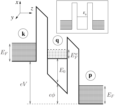
Figure 2: Schematic potential profile of the double-barrier resonant tunneling structure. The structure consists of a quantum well separated from two leads by tunneling barriers. The electrons with three-dimensional wavevectors $\mathbf{k}$ and $\mathbf{p}$ fill all the states up to the Fermi energies $E_{F}$ in the left and right leads, respectively. In the quantum well the motion of electrons in the $z$-direction is quantized, and the electrons with two-dimensional transverse wavevectors $\mathbf{q}$ occupy all the states up to the Fermi energy $E_{F}^{w}$. The inset shows the potential profile at zero bias.

The electric current in the device fluctuates, because the electrons tunnel in and out of the well at random moments in time. The resulting shot noise of current through the heterostructure gives rise to the metastability of some current states. The two solid lines in Fig. 1 correspond to the most probable values of current at a given bias. These two branches are stable, i.e., any small fluctuation of current near a solid line will decay with time, and the current will return to its value at the solid line. The dashed line between ${\widetilde{V}}_{th}$ and $V_{th}$ corresponds to the unstable state. Here any deviation from the dashed line which raises or lowers the current will switch the system to the upper or lower stable current state, respectively.

Qualitative understanding of the metastability can be achieved by considering the system at a bias near $V_{th}$, e.g., point M on the upper branch of the $I$-$V$ curve, Fig. 1. Then, as one can see from Fig. 1, a relatively small fluctuation can shift the current below the dashed line corresponding to the unstable state. If that happens, the system switches to the lower branch. The opposite process is much less probable, since the distance from the lower branch to the dashed line is much larger than that from the upper branch. Therefore, the lower branch is stable, and the system remains in that state.

The dependence of the mean switching time $\tau$ on the bias was addressed theoretically in Ref. paper1, . It was shown that near the threshold voltage $V_{th}$ the logarithm of $\tau$ behaves as

$$\ln\tau\propto\left\{\begin{array}[]{ll}(V_{th}-V)^{3/2},&L\ll r_{0},\\ V_{th}-V,&L\gg r_{0}.\end{array}\right.$$ (1)

Here $L$ is the size of the sample, $r_{0}\propto\sigma^{1/2}(V_{th}-V)^{-1/4}$ is a characteristic length scale, and $\sigma$ is the in-plane conductivity. In small samples, $L\ll r_{0}$, the current switches from the metastable state to the stable one simultaneously over the entire area of the device. On the other hand, in large samples, $L\gg r_{0}$, the switching is initiated in a small critical region of radius $r_{0}$. After the switching has occurred in that region, it extends rapidly to the rest of the sample.

In this paper we show that if the sample is large, the switching can initiate not only inside, but also at the edge of the device. The latter process tends to be more efficient, since the exponential in the respective expression for $\tau$ is smaller than in the case of switching far from the edges of the sample (Sec. V). On the other hand, the switching at the edge can be initiated anywhere along the boundary of the device, and thus the prefactor of the switching rate $1/\tau$ due to these processes is proportional to the perimeter $\sim L$. Similarly, the prefactor of the rate of switching inside the device is proportional to the area $\sim L^{2}$, which makes these processes more efficient in larger samples.

We obtain analytically the full expressions for $\tau$, including the preexponential factors. Apart from the dependence on sample dimensions, the calculation of the prefactors reveals the non-trivial dependence of the threshold voltage $V_{th}$ on the degree of disorder of the sample. Formal evaluation of the prefactors in the case of non-uniform electron density in the well results in ultraviolet divergences. Similar divergences appear in quantum field theory, where they are eliminated with the use of a renormalization procedure. ZinnJustin ; Coleman1 The application of a similar technique to our problem leads to the renormalization of the threshold voltage which depends strongly on the conductivity of the quantum well (Secs. IV.1.2, V). Upon this renormalization $\ln\tau$ in large samples acquires logarithmic corrections to its linear voltage dependence.

The paper is organized as follows. In Sec. II we obtain the Fokker-Planck equation for tunneling in DBRTS which completely describes the electron transport in small samples. This equation enables us to find a simple result for the mean switching time in these samples. In Sec. III we derive the Fokker-Planck equation for the case of large samples which describes the dynamics of electron density in the well due to both the diffusion in the plane of the well and tunneling between the well and the leads. We use it to investigate the effect of weak density fluctuations on the decay of metastable current state in small samples (Sec. IV) and to study the switching in large samples (Sec. V). The application of our theory to the existing and future experiments is discussed in Sec. VI.

II Fokker-Planck equation for tunneling in DBRTS

The bistable current-voltage characteristic of DBRTS was studied theoretically in Refs. Sheard88, ; numerical89, ; Anda93, ; Blanter99, . The $I$-$V$ curve shows the dependence of the average current on voltage applied to the device. In addition, shot noise was studied in the regime of small fluctuations. numerical89 ; Anda93 ; Blanter99 On the other hand, the switching between the branches of the $I$-$V$ curve is caused by large fluctuations of current. In this section we use the model of Ref. Blanter99, to derive the Fokker-Planck equation for tunneling in DBRTS, which accounts for these large fluctuations, and thus describes the switching.

The model is illustrated in Fig. 2. The well is extended in $x$-$y$ plane. The motion in $z$-direction in the well is quantized, and the well is assumed to have only one resonant level of energy $E_{0}$. The two-dimensional wavevectors in the well are denoted by $\mathbf{q}$. The left and right leads are three-dimensional; the wavevectors of electrons are denoted by $\mathbf{k}$ and $\mathbf{p}$, respectively. The conduction bands in the leads are occupied up to the Fermi energy $E_{F}$. In typical devices $E_{0}$ is of the order of $E_{F}$; for definiteness we assume $E_{0}>E_{F}$. The temperature $T$ is assumed to be small compared to $E_{F}$ and $eV$. The well is separated from the leads by two tunneling barriers with the transmission coefficients much smaller than unity.

In Ref. Blanter99, the tunneling through the double barrier was described quantum-mechanically using the Breit-Wigner formula. The level widths with respect to the decay to the right and left leads $\Gamma_{L}$, $\Gamma_{R}$ there were eventually taken to be much smaller than all other relevant energy scales. We make this assumption from the beginning, and describe the electron transport through the barriers using the sequential tunneling approach. This method is an alternative to the use of the Breit-Wigner formula; it enables us to discuss both the $I$-$V$ characteristic and the large fluctuations of current.

In order to have a steady state of non-zero current in the device, the electrochemical potential in the well should lie between those in the left and right leads, i.e.,

$$eV+E_{F}>E_{0}+e\phi+E_{F}^{w}>E_{F}.$$ (2)

Here $E_{F}^{w}=\hbar^{2}q_{F}^{2}/2m$ is the Fermi energy in the well with $m$ being the effective mass. Then, in the limit of low temperature the inequalities (2) dictate that the tunneling is possible only in one direction, namely, from left to right, Fig. 2. The probability to tunnel through a barrier is given by the Fermi golden rule. The rates of electron tunneling into the well $J_{L}$ and out of the well $J_{R}$ take the form:

$$J_{L} = \frac{4\pi}{\hbar}\sum_{\mathbf{qk}}|t_{k_{z}}|^{2}\delta_{\mathbf{qk}_{\parallel}}f_{\mathbf{k}}(1-f_{\mathbf{q}})$$ (3)

$$\times\delta(eV+E(k_{z})-E_{0}-e\phi),$$

$$J_{R} = \frac{4\pi}{\hbar}\sum_{\mathbf{qp}}|t_{p_{z}}|^{2}\delta_{\mathbf{qp}_{\parallel}}f_{\mathbf{q}}\delta(E_{0}+e\phi-E(p_{z})).$$ (4)

Here $E(k)=\hbar^{2}k^{2}/2m$; $f_{\mathbf{k}}$ and $f_{\mathbf{q}}$ are the Fermi occupation numbers in the left lead and the quantum well, respectively. In Eq. (4) we used the fact that the Fermi occupation numbers in the right lead $f_{\mathbf{p}}=0$ at energies above $E_{0}+e\phi$, because $E_{0}>E_{F}$. Expressions (3), (4) include an additional factor of $2$, which accounts for electron spins. The matrix elements $t_{p_{z}}$ ($t_{k_{z}}$) describe the transitions between the resonant level in the well and the state with $z$-component of the wavevector $p_{z}$ ($k_{z}$) in the right (left) lead. The conservation of the transverse momentum is taken into account by Kronecker deltas.

To simplify the expression for the tunneling rate (4) we use $\delta_{\mathbf{qp}_{\parallel}}$ to remove the sum over $\mathbf{p}_{\parallel}$. The remaining sum over $\mathbf{q}$ of Fermi function $f_{\mathbf{q}}$ gives exactly the number of electrons in the well with a given spin $N/2$. Then Eq. (4) reduces to

$$J_{R}=\frac{\Gamma_{R}}{\hbar}N.$$ (5)

Here $\Gamma_{R}$ is the level width with respect to tunneling into the right lead. We define the level widths for the two possible tunneling processes as

$$\Gamma_{L} = 2\pi\sum_{k_{z}}|t_{k_{z}}|^{2}\delta(eV+E(k_{z})-E_{0}-e\phi),$$ (6a)

$$\Gamma_{R} = 2\pi\sum_{p_{z}}|t_{p_{z}}|^{2}\delta(E_{0}+e\phi-E(p_{z})).$$ (6b)

To find $J_{L}$ we use the Kronecker delta to remove the sum over $\mathbf{k}_{\parallel}$ in Eq. (3), while the value of $k_{z}^{2}=(2m/\hbar^{2})(E_{0}+e\phi-eV)$ is fixed by the delta function. At $\mathbf{k}=(\mathbf{q},k_{z})$ and $T\to 0$ the sum over $\mathbf{q}$ of $f_{\mathbf{k}}(1-f_{\mathbf{q}})$ can be easily evaluated, and gives $(S/4\pi)(k_{F}^{2}-k_{z}^{2}-q_{F}^{2})$ under the condition (2), where $S$ is the area of the sample. Then, the expression (3) can be simplified as follows

$$J_{L}=\frac{\Gamma_{L}}{\hbar}\left[\frac{Sm}{\pi\hbar^{2}}(E_{F}+eV-E_{0}-e\phi)-N\right].$$ (7)

Here we used the expression $N=Sq_{F}^{2}/2\pi$ for the total number of electrons in the well. Note that at $eV>e\phi+E_{0}$ the level width (6a) vanishes, and thus $J_{L}=0$.

In the sequential tunneling approximation the average number of electrons in the well can be determined from the condition $J_{L}=J_{R}$,

$$N=\frac{Sm}{\pi\hbar^{2}}\frac{\Gamma_{L}}{\Gamma_{L}+\Gamma_{R}}(E_{F}+eV-E_{0}-e\phi).$$ (8)

One cannot directly obtain $N$ from Eq. (8), since the potential $\phi$ depends on the number of electrons in the well. Considering the barriers as two capacitors, one finds from electrostatics the following expression for the electric potential of the well (Fig. 2),

$$\phi=\frac{V}{2}+\frac{eN}{2C}.$$ (9)

Here we assumed for simplicity that the capacitances of the left and right barriers are equal to each other, and denoted the capacitance of each barrier as $C$.

One can obtain the current-voltage characteristic of the DBRTS by repeating the following steps of Ref. Blanter99, . First, one notices that the level widths are energy dependent:

$$\Gamma_{L} = g_{L}\sqrt{E_{0}(E_{0}-eV+e\phi)},$$ (10a)

$$\Gamma_{R} = g_{R}\sqrt{E_{0}(E_{0}+e\phi)},$$ (10b)

where $g_{L,R}$ are dimensionless constants. Since $\Gamma_{L}$ and $\Gamma_{R}$ depend on $\phi$, they are also functions of $N$. Therefore to find $N$ one has to solve the pair of equations (8) and (9). The latter leads to an equation on $N$, which has three solutions in the bistable region. One of the solutions corresponds to the average number of electrons on the unstable branch, while the other two correspond to $N$ on the lower ($N=0$) and upper stable branches. Upon substitution of $N$ into Eq. (5) one finds the dependence of the average current on bias, i.e., the bistable $I$-$V$ curve, Blanter99 which is schematically shown in Fig. 1.

To account for the noise, we go one step further and write the master equation for the time evolution of the distribution function $P(N,t)$ of the number of electrons in the well $N$. In terms of the tunneling rates (3) and (4), the master equation for $P(N,t)$ takes the form

$$\frac{\partial}{\partial t}P(N,t) = P(N-1,t)J_{L}(N-1)$$ (11)

$$+P(N+1,t)J_{R}(N+1)$$

$$-P(N,t)[J_{L}(N)+J_{R}(N)].$$

The first two terms in the right-hand side of Eq. (11) account for the processes which increase the probability to have $N$ electrons in the well, while the last term corresponds to the opposite processes.

In this section we consider the samples of large in-plane conductivity where the density in the well is uniform. Therefore, in the steady state of non-zero current the total number of particles in the well is proportional to the area of the sample. The linear dimensions of the sample are assumed to be large compared to the Bohr radius in the semiconductor. Thus the total number of electrons in the well is large, $N\gg 1$, and one can expand Eq. (11) in $1/N$. Keeping the terms up to the second order, the master equation reduces Landauer62 to

$$\frac{\partial}{\partial t}P(N,t)=-\frac{\partial}{\partial N}[A(N)P(N,t)]+\frac{1}{2}\frac{\partial^{2}}{\partial N^{2}}[B(N)P(N,t)].$$ (12)

Here $A(N)=J_{L}(N)-J_{R}(N)$ and $B(N)=J_{L}(N)+J_{R}(N)$. Equation (12) is known as the Fokker-Planck equation, and is widely used for the description of various stochastic processes, see, e.g., Refs. vanKampen, ; Gardiner, .

The stationary solution of Eq. (12) can be easily obtained:

$$P_{0}(N)=\frac{\mbox{const}}{B(N)}e^{-U(N)},\quad U(N)=-2\int_{0}^{N}\frac{A(N^{\prime})}{B(N^{\prime})}\,dN^{\prime},$$ (13)

Ref. vanKampen, . The extrema of function $U(N)$ are determined by the condition $A\equiv J_{L}-J_{R}=0$, which we used above to find the average current through the device. Therefore each extremum of $U(N)$ corresponds to one of the branches of the $I$-$V$ curve. Outside the bistable region the current $I(V)$ is uniquely defined, and $U(N)$ has a single minimum. In the bistable region $U(N)$ has two minima and a maximum, which correspond to the locally stable current branches and the unstable branch, respectively [Fig. 1].

From the definitions of $A$ and $B$, it is clear that their ratio is independent of the area of the sample $S$. Using the expression (13) and the fact that $N\propto S$, one can see that $U$ is linearly proportional to $S$. Thus $U(N)$ is an extensive quantity, and its dependence on $N$ and $S$ has the general form $U(N,S)=Su(n)$, where $n=N/S$ is the electron density. Since the area of the sample is large, we have $U\gg 1$. Therefore, the distribution function $P_{0}$ is peaked sharply near the global minimum of $U(N)$.

The experiments Grahn96 ; Grahn98 ; Teitsworth studying the switching between the branches of the $I$-$V$ curve are set up as follows. One starts at $V<{\widetilde{V}}_{th}$, Fig. 1, where only one value of current is possible. In this case $U(N)$ has only one minimum, as shown schematically by the dash-dotted line in Fig. 3a. If we increase the bias up to some value slightly above ${\widetilde{V}}_{th}$, the function $U(N)$ will acquire a new minimum to the left of the old one, see the dashed line in Fig. 3a. This corresponds to the appearance of the lower current branch of the $I$-$V$ curve. The new minimum is a local one, and the main peak of the distribution function is still centered at the old minimum. Thus, the system remains on the upper branch of the $I$-$V$ curve. Further increasing $V$, we transform $U(N)$ to the shape shown schematically by the solid line in Fig. 3a. Here the right minimum of $U(N)$ is a local one, and if we leave the system in this state for a sufficiently long time, it will eventually switch to the left minimum. To switch from the local minimum to the global one, the system has to overcome the barrier of height $U_{b}$, Fig. 3a. From the form of the distribution function (13) it is clear that this process takes a long time $\tau\propto\exp(U_{b})$. To perform the measurement of the switching time from the upper to the lower current branch, one increases the bias to the chosen value over a time short compared to $\tau$, and then waits until the system switches to the lower branch.

Figure 3: (a) Generic behavior of $U(N)$ at different values of bias. Outside the bistable region $U(N)$ has one minimum (top curve). Inside the bistable region the function $U(N)$ has two minima and a maximum, which correspond to the locally stable current branches and the unstable branch, respectively (middle and bottom curves). (b) The sketch of $U(N)$ for the model of Fig. 1. Solid line corresponds to a bias slightly below $V_{th}$, whereas dashed line depicts $U(N)$ for the bias slightly above ${\widetilde{V}}_{th}$.

At the threshold the right minimum of $U(N)$ disappears, and $U_{b}=0$. Since $U(N)$ is an extensive quantity, $U_{b}$ grows rapidly when we move from the threshold into the bistable region, and the switching time becomes very long. Therefore, in order for the switching to occur within a reasonable timeframe, the system should be close to the threshold.

As the voltage approaches its threshold value, the maximum at $N_{\text{max}}$ and the local minimum of $U(N)$ at $N_{\text{min}}$ (Fig. 3) move closer to each other, and at the threshold they coincide. At this point one can define a threshold electron density $n_{th}\equiv N_{\text{max}}/S=N_{\text{min}}/S$. In the vicinity of $n=n_{th}$ and $V=V_{th}$ the function $u(n)$ can be approximated by a cubic polynomial,

$$u(n)\approx-\alpha(n-n_{th})+\frac{\gamma}{3}(n-n_{th})^{3}+u_{th},\quad\alpha=a(V_{th}-V).$$ (14)

Here the constant $u_{th}$ is the value of $u$ at $n=n_{th}$ and $V=V_{th}$.

To derive Eq. (14) microscopically, one has to consider $A(N)$ and $B(N)$ on the upper branch of the $I$-$V$ curve in the vicinity of the threshold $V_{th}$. An analytical calculation of $I(V)$ is possible Blanter99 if the dimensionless parameter

$$\lambda=\frac{me^{2}}{2\pi\hbar^{2}c}$$ (15)

is small, $\lambda\ll 1$. Here $c=C/S$ is the capacitance per unit area. In Appendix A we extend this approach to find $A(N)$, $B(N)$, and the coefficients of expansion (14) at $\lambda\ll 1$.

The expansion (14) can be justified for any $\lambda$ in the spirit of the Landau theory of second-order phase transitions. LandauStat1 The potential $u$ is expected to be an analytic function of $n$ and $V$. Thus, $u$ can be expanded in Taylor series near the threshold, with $n-n_{th}$ playing the role of the order parameter. Since the local minimum and the maximum of $u$ coincide at the threshold, both the first and second derivatives of $u(n)$ vanish at $V=V_{th}$ and $n=n_{th}$. Therefore, the expansion starts with the third-order term. The sign of $\gamma$ is not important; we choose $\gamma>0$, which corresponds to the behavior of $U$ near the right minimum as shown in Fig. 3a. At $V\neq V_{th}$, the linear $\alpha(n-n_{th})$ and quadratic $\frac{1}{2}\beta(n-n_{th})^{2}$ terms are also present. Since $\alpha=\beta=0$ at $V=V_{th}$, we expect $\alpha\propto(V_{th}-V)$, $\beta\propto(V_{th}-V)$. We keep only the linear term in the expansion, because the second-order term is quadratic in small parameter $n-n_{th}$, and therefore is small compared to the linear one. In order for $u$ to have a local minimum at $V<V_{th}$, the coefficient $a$ should be positive.

Near the threshold the function $B(N)$ can be approximated by a constant,

$$B(N_{th})=2J_{R}=2\Gamma_{R}N_{th}/\hbar.$$ (16)

In the case of constant $B$ the Fokker-Planck equation (12) has been studied in detail. In particular, the exact expression for the mean switching time can be obtained including the prefactor (Ref. vanKampen, , Sec. XIII.2). In our notations it reads

$$\tau=\frac{4\pi}{B\sqrt{U^{\prime\prime}(N_{\text{min}})|U^{\prime\prime}(N_{\text{max}})|}}\exp(U_{b}).$$ (17)

For the potential (14) one can easily find the barrier height, $U_{b}=4S\alpha^{3/2}/3\gamma^{1/2}$. The prefactor of Eq. (17) can be also straightforwardly evaluated, and one obtains the following expression for the mean switching time,

$$\tau=\frac{2\pi}{b\sqrt{\alpha\gamma}}\exp\left[\frac{4}{3}\frac{S[a(V_{th}-V)]^{3/2}}{\gamma^{1/2}}\right],$$ (18)

where $b=B/S$ is independent of the area of the sample. This result obviously agrees with Eq. (1) for small samples ($L\ll r_{0}$).

Expansion (14) is quite generic, and similar theoretical results were found in many different areas of physics. Kurkijarvi ; Victora ; Dykman1 ; Dykman2 ; Dykman:exp ; Dykman3 ; Dykman4 In particular, Eq. (12) is also used to describe the motion of a Brownian particle in external potential, where $N$ plays the role of the coordinate of the particle. Therefore, the logarithm of the mean escape time of the Brownian particle from a local minimum of potential is also expected to obey the $3/2$-power law. Recently this behavior of the escape time was confirmed experimentally for the optically trapped Brownian particle. Dykman:exp

The lower branch of the $I$-$V$ curve corresponds to the situation where the level in the well $E_{0}+e\phi$ is below the bottom $eV$ of the conduction band in the left lead. In this case $J_{L}\equiv 0$ and $B=-A=J_{R}$. Consequently, as $N\to 0$ we have $U(N)=2N$, see Eq. (13). Since $N$ cannot be negative, $U$ reaches its minimum at the boundary $N=0$ of the range of allowed values of $N$, where the derivative $U^{\prime}(N)\neq 0$, Fig. 3b. The non-analyticity of $U(N)$ near the left minimum does not affect the calculation of the time of switching from upper to the lower branch. Indeed, at a bias slightly below $V_{th}$, the function $U(N)$ is analytic near its maximum and the local minimum (solid line in Fig. 3b), and the description of the switching from the upper to the lower branch in terms of Eqs. (14) and (17) is correct. However, the situation is different for the switching from the lower to the upper branch of the $I$-$V$ curve. To study this process, we decrease the bias to the value slightly above ${\widetilde{V}}_{th}$. The function $U(N)$ for this case is depicted schematically by the dashed line in Fig. 3b. Here $U(N)$ is non-analytic at its local minimum, and therefore we cannot use expressions (14) and (17) for the switching time. The non-analytic behavior of $U(N)$ is a consequence of crudeness of our model, in which the current on the lower branch is exactly zero. On the other hand, the experimentally measured $I$-$V$ curves show non-zero current on the lower branch. Thus, in a more detailed model which accounts for this non-zero current, the minimum corresponding to the lower branch of the $I$-$V$ curve will be reached at non-zero $N$. The discussion based on Eqs. (14) and (17) will then be valid.

III Fokker-Planck equation for transport in DBRTS of large area

In section II we studied the decay of a metastable state in DBRTS under the assumption that the electron density in the quantum well is uniform. Then the switching time $\tau$ given by Eq. (18) grows exponentially with the area of the sample. Since electrons can tunnel at any point of the quantum well, the tunneling process creates a non-uniform electron density. On the other hand, the diffusion of particles in the well leads to spreading of the charge across the sample. In small samples the spreading is fast, and the density becomes uniform. In samples of large area the electron density may change significantly before the charge spreads over the entire well. In this case the switching between the two branches of the $I$-$V$ curve is initiated in a small part of the sample, and the switching time is not exponential in the area $S$.

In this section we generalize the Fokker-Planck equation (12) to the case of non-uniform density ${n({\bf r})}$, where $\textbf{r}=(x,y)$ is a position in the well. In subsequent sections this equation will be used to study the decay of a metastable state in DBRTS of large area.

III.1 Equation for distribution function of electron density in an isolated quantum well

We begin by considering the simplest case of a quantum well not coupled to the leads. At finite temperature the electron density in the well fluctuates and can be described by a distribution function $P\{n(\mathbf{r}),t\}$. Here we derive the Fokker-Planck equation for the distribution function of electron density due to the in-plane diffusion of electrons in the well. In section III.2 we add the tunneling through the barriers and obtain the Fokker-Planck equation for DBRTS of large area.

We consider density fluctuations at length scales much greater than the inelastic mean free path. These density fluctuations are slow in comparison with the energy relaxation time in the well. Therefore the system is in a local equilibrium, and the distribution of electrons at any point in the well is given by a Fermi function. Note that the chemical potential in this Fermi function is determined by the electron density, and therefore varies from point to point following the dependence $n(\mathbf{r})$.

Let us choose a time interval $\Delta t$ much smaller than the relaxation time for $P\{n(\mathbf{r}),t\}$ and large in comparison with the collision time, so that the motion of electrons can be treated as diffusive. Then one can write the following equation for the evolution of the distribution function,

$$P\{n(\mathbf{r}),t+\Delta t\}-P\{n(\mathbf{r}),t\}=\int\!\!\int d\mathbf{r}_{1}d\mathbf{r}_{2}$$

$$\times\Big{[}P\{n(\mathbf{r})+\delta n_{12}(\mathbf{r}),t\}W_{\Delta t}(\mathbf{r}_{1},\mathbf{r}_{2};n(\mathbf{r})+\delta n_{12}(\mathbf{r}))$$

$$-P\{n(\mathbf{r}),t\}W_{\Delta t}(\mathbf{r}_{2},{\bf r}_{1};n(\mathbf{r}))\Big{]}.$$ (19)

Here $\delta n_{12}({\bf r})=\delta({\bf r}-{\bf r}_{1})-\delta({\bf r}-{\bf r}_{2})$ is the correction to the density $n(\mathbf{r})$ due to the displacement of one electron from point $\mathbf{r}_{2}$ to $\mathbf{r}_{1}$; the probability density $W_{\Delta t}({\bf r}_{1},{\bf r}_{2};n(\mathbf{r}))$ describes diffusion of an electron from a point ${\bf r}_{1}$ in the quantum well to point ${\bf r}_{2}$ during the time interval $\Delta t$. Since the diffusion rate may depend on the electron density, $W_{\Delta t}$ is a functional of $n(\mathbf{r})$.

Expanding the first term in the right-hand side of Eq. (III.1) up to the second order in $\delta n_{12}({\bf r})$, one obtains the following equation:

$$\Delta P\{n,t\} = \frac{1}{2}\int\!\!\int d{\bf r}_{1}d{\bf r}_{2}\left\{\left(\frac{\delta}{\delta n({\bf r}_{1})}-\frac{\delta}{\delta n({\bf r}_{2})}\right)\right.$$ (20)

$$\times[W_{\Delta t}({\bf r}_{1},{\bf r}_{2};n)-W_{\Delta t}({\bf r}_{2},{\bf r}_{1};n)]$$

$$+\frac{1}{2}\left(\frac{\delta}{\delta n({\bf r}_{1})}-\frac{\delta}{\delta n({\bf r}_{2})}\right)^{2}[W_{\Delta t}({\bf r}_{1},{\bf r}_{2};n)$$

$$+W_{\Delta t}({\bf r}_{2},{\bf r}_{1};n)]\bigg{\}}P\{n,t\}.$$

The probability densities $W_{\Delta t}$ to diffuse from $\mathbf{r}_{1}$ to $\mathbf{r}_{2}$ and back are not independent,

$$W_{\Delta t}({\bf r}_{1},{\bf r}_{2};n)e^{-\mu_{1}/T}=W_{\Delta t}({\bf r}_{2},{\bf r}_{1};n)e^{-\mu_{2}/T}.$$ (21)

Here $\mu_{1}$ and $\mu_{2}$ are the electrochemical potentials at points $\mathbf{r}_{1}$ and ${\bf r}_{2}$, respectively. For the case of elastic scattering by impurities considered in Ref. paper1, expression (21) directly follows from Eq. (8) of Ref. paper1, . Generalization of Eq. (21) to arbitrary scattering mechanism is discussed in Appendix B.

In order to find $\mu$ we need to account for the interactions between electrons. We limit ourselves to the charging energy approximation; the electron exchange and correlation effects are neglected. Then at low temperatures $T\ll E_{F}$, the values of the electrochemical potential are found by adding the electrostatic potential $e^{2}n/c$ to the Fermi energy,

$$\mu_{1,2}=\frac{e^{2}}{\tilde{c}}n({\bf r}_{1,2}).$$ (22)

Here the effective capacitance per unit area $\tilde{c}$ is defined by $e^{2}/{\tilde{c}}=e^{2}/{c}+1/{\nu}$, and $\nu$ is the density of states in the well.

In short time $\Delta t$ an electron can only diffuse over a short distance, so that $|\mu_{1}-\mu_{2}|\ll T$. Therefore using Eq. (21), one can expand the expression in the curly brackets in the right-hand side of Eq. (20) to the leading order in $(\mu_{1}-\mu_{2})/T$, and with the help of Eq. (22) obtain

$$\Delta P\{n,t\} = \frac{1}{2}\int\!\!\int\!\!d{\bf r}_{1}d{\bf r}_{2}\Bigg{\{}\frac{e^{2}}{{\tilde{c}}T}\left(\frac{\delta}{\delta n({\bf r}_{1})}-\frac{\delta}{\delta n({\bf r}_{2})}\right)$$ (23)

$$\!\left.\times[n({\bf r}_{1})-n({\bf r}_{2})]+\left(\frac{\delta}{\delta n({\bf r}_{1})}-\frac{\delta}{\delta n({\bf r}_{2})}\right)^{2}\right\}$$

$$\times W_{\Delta t}({\bf r}_{1},{\bf r}_{2};n)P\{n,t\}.$$

To proceed further we need an expression for the transition probability density $W_{\Delta t}$. This quantity is affected by all the relevant processes of electron scattering, such as elastic scattering of electrons by impurities, electron-phonon and electron-electron scattering. Instead of accounting for all these processes explicitly, we express $W_{\Delta t}$ in terms of in-plane conductivity $\sigma$, which can in principle be measured experimentally. Assuming that electron motion is diffusive, we conclude that the average square of the distance traveled by an electron during a short time interval is proportional to $\Delta t$, i.e.,

$$\int\!\!W_{\Delta t}({\bf r}_{1},{\bf r}_{2};n)|{\bf r}_{1}-{\bf r}_{2}|^{2}\,d{\bf r}_{2}=G\Delta t.$$ (24)

Here the constant $G$ is proportional to the conductivity, $G=4T\sigma/e^{2}$, see Appendix C.

At small $\Delta t$ the transition probability density $W_{\Delta t}$ can be expanded as

$$W_{\Delta t}({\bf r}_{1},{\bf r}_{2};n)=\delta({\bf r}_{1}-{\bf r}_{2})+\frac{T\sigma\Delta t}{e^{2}}\nabla^{2}\delta({\bf r}_{1}-{\bf r}_{2})+\dots~{}.$$ (25)

The physical meaning of the first term in this expansion is that electron remains at its initial position $\mathbf{r}_{1}$ at $\Delta t=0$. Thus the second term is needed to account for the electron diffusion. The coefficient in the second term is found by applying the expansion (25) to Eq. (24).

Equation (23) can be simplified significantly using expansion (25), and eventually takes the form

$$\frac{\partial}{\partial t}P\{n,t\}=-\frac{\sigma}{e^{2}}\int\!\!d{\bf r}\,\frac{\delta}{\delta n}\left[\frac{e^{2}}{\tilde{c}}\nabla^{2}n+T\nabla^{2}\frac{\delta}{\delta n}\right]P\{n,t\}.$$ (26)

This is the Fokker-Planck equation for the evolution of the distribution function of electron density. The first term in Eq. (26) describes the spreading of the charge in the well, whereas the second term accounts for the thermal noise.

It is instructive to substitute into Eq. (26) the equilibrium distribution function $P_{0}\{n\}$. The latter has the Gibbs form $e^{-E/T}$, namely,

$$P_{0}\{n\}=\exp\left[-\frac{1}{T}\int\frac{e^{2}n^{2}({\bf r})}{2\tilde{c}}\,d{\bf r}\right].$$

Here the energy per unit area $\varepsilon={e^{2}n^{2}}/{2{\tilde{c}}}$ is chosen in a way that reproduces the electrochemical potential $\mu=\partial\varepsilon/\partial n$ in the form (22). It is easy to check that $P_{0}\{n\}$ satisfies the Fokker-Planck equation (26).

III.2 Combined Fokker-Planck equation for tunneling and diffusion

In this section we obtain the combined Fokker-Planck equation which incorporates both the tunneling through the barriers and diffusion inside the well. We begin by generalizing the tunneling Fokker-Planck equation (12) to the case of non-uniform electron density. This is accomplished by dividing the plane of the well into small pieces, so that the density is uniform within each piece. In the absence of in-plane diffusion, the distribution function of electron density in the entire plane is given by the product of distribution functions of its pieces, $P=\prod_{j}P_{j}\{N_{j}\}$. Applying Eq. (12) to each piece we obtain the following Fokker-Planck equation for the distribution function of the entire quantum well,

$$\frac{\partial}{\partial t}P=\sum_{j}\frac{\partial}{\partial N_{j}}\left[-A(N_{j})+\frac{1}{2}\frac{\partial}{\partial N_{j}}B(N_{j})\right]P.$$

The functions $A(N_{j})$ and $B(N_{j})$ are extensive quantities, and it is convenient to rewrite them as $A(N_{j})=\Delta Sa(n)$ and $B(N_{j})=\Delta Sb(n)$, where $\Delta S$ is the area of each piece. Replacing the sum with the integral over the area of the sample and $\partial/\partial N_{j}$ with the functional derivative $\delta/\delta n(\mathbf{r}_{j})$, we find the continuous form of this equation:

$$\frac{\partial}{\partial t}P\{n,t\}=\!\int\!\!d\mathbf{r}\frac{\delta}{\delta n}\left[-a(n(\mathbf{r}))+\frac{1}{2}\frac{\delta}{\delta n}b(n(\mathbf{r}))\right]P\{n,t\}.$$ (27)

Let us now take into account the in-plane diffusion of electrons, which was discussed in Sec. III.1. Because the tunneling and diffusion are independent processes, we can add the right-hand sides of Eqs. (27) and (26) and obtain the combined Fokker-Planck equation for DBRTS of large area:

$$\frac{\partial}{\partial t}P\{n,t\} = \int\!\!d\mathbf{r}\,\frac{\delta}{\delta n}\left[-a(n)+\frac{1}{2}\frac{\delta}{\delta n}b(n)\right.$$ (28)

$$\left.-\frac{\sigma}{\tilde{c}}\nabla^{2}n-T\frac{\sigma}{e^{2}}\nabla^{2}\frac{\delta}{\delta n}\right]P\{n,t\}.$$

This equation generalizes Eq. (26) to the case of a quantum well coupled to the leads.

In the vicinity of the threshold $V_{th}$ the function $b(n)$ can be approximated by a constant $b=b(n_{th})$. In addition, one can substitute $2a/b=2A/B=-u^{\prime}(n)$, c.f. Eq. (13). At bias near $V_{th}$ the function $u(n)$ is given by the approximate expression (14), and Eq. (28) can be rewritten as

$$\frac{\partial}{\partial t}P\{n,t\} = \frac{b}{2}\int\!\!d\mathbf{r}\,\frac{\delta}{\delta n}\bigg{[}-\alpha+\gamma(n-n_{th})^{2}$$ (29)

$$\left.-2\eta\nabla^{2}n+\frac{\delta}{\delta n}\right]P\{n,t\},$$

where we defined $\eta=\sigma/{\tilde{c}}b$. In Eq. (29) we omitted the term proportional to the temperature, since it is negligible at low $T$. (The exact criterion is discussed in Appendix D.) Thus from now on we study only the effect of the shot noise due to the tunneling of electrons at high bias $eV\gg T$, whereas the thermal noise is neglected.

The stationary solution of Eq. (29) is found by setting the left-hand side to zero,

$$P_{0}\{n\} = e^{-F\{n\}},$$

$$F\{n\} = \int\!\!d{\bf r}\left[-\alpha(n-n_{th})+\frac{\gamma}{3}(n-n_{th})^{3}+\eta(\nabla n)^{2}\right].$$

The functional $F\{n\}$ has two contributions: the first two terms account for the tunneling, and the remaining term is due to the in-plane diffusion.

The functional $F\{n\}$ is similar to the free energy in Ginzburg-Landau theory of phase transitions, with $n-n_{th}$ playing the role of the order parameter. For the case of uniform electron density in the well, $\nabla n=0$, the functional $F\{n\}$ coincides with Eq. (13). If the density is non-uniform, the gradient term $(\nabla n)^{2}$ appears in the expansion in addition to the terms from Eq. (13). This gradient term suppresses large variations of the electron density.

III.3 Dimensionless Fokker-Planck equation

For the following discussion it is convenient to parametrize the electron density $n(\mathbf{r})$ in terms of a dimensionless function $z(\bm{\rho})$ that vanishes at the minimum of $u(n)$,

$$n({\bf r}) = n_{min}-2\sqrt{\frac{\alpha}{\gamma}}\,z({\bf r}/r_{0}),$$ (31a)

$$r_{0} = \frac{\sqrt{\eta}}{(\alpha\gamma)^{1/4}}=\sqrt{\frac{\sigma}{{\tilde{c}}b\sqrt{\alpha\gamma}}}.$$ (31b)

Here the density at the minimum $n_{min}=n_{th}+\sqrt{\alpha/\gamma}$ can be easily found from Eq. (14). The Fokker-Planck equation (29) in terms of $z(\bm{\rho})$ takes the form:

$$\frac{\partial P\{z,t\}}{\partial t} = b\sqrt{\gamma\alpha}\int\!\!d\bm{\rho}\,\frac{\delta}{\delta z}\left[-\nabla_{\rho}^{2}z+z-z^{2}+\frac{1}{U_{0}}\frac{\delta}{\delta z}\right]$$ (32)

$$\times P\{z,t\},$$

where

$$U_{0}=\frac{8\eta\alpha}{\gamma}.$$ (33)

The stationary solution $P_{0}$ of Eq. (32) is given by

$$P_{0}\{z\}=e^{-F},\qquad F=U_{0}\int\!\!d\bm{\rho}\left[\frac{(\nabla_{\rho}z)^{2}}{2}+\frac{z^{2}}{2}-\frac{z^{3}}{3}\right].$$ (34)

One can see that the characteristic value of the functional $F$ is given by $U_{0}$, whereas the characteristic size $r_{0}$ plays the role of a typical length scale of stochastic fluctuations of electron density $n(\mathbf{r})$.

IV Decay of the metastable state in extended samples

In Sec. II we obtained the expression for the mean switching time in DBRTS under the assumption of uniform electron density in the well. This assumption is valid only if the dimensions of the sample are small compared to the length scale $r_{0}$ of the density fluctuations, Eq. (31b). If the sample is large, the fluctuations of electron density must be taken into account.

In Sec. III we obtained the Fokker-Plank equation (29) which describes the time evolution of the distribution function of electron density. Unlike Eq. (12) for the case of uniform density, this equation has an infinite number of variables, since the density is different at every point.

The most general form of the multidimensional Fokker-Planck equation is

$$\!\!\!\!\!\frac{\partial P({\bf x},t)}{\partial t} = {\cal L}\,P({\bf x},t),$$

$${\cal L} = -\sum\limits_{i}\frac{\partial}{\partial x_{j}}K_{i}(\mathbf{x})+\sum\limits_{i,j}\frac{\partial^{2}}{\partial x_{i}\partial x_{j}}D_{ij}({\bf x}).$$ (35)

Assuming that the system has a metastable state, one can consider its domain of attraction $\Omega$. The domain boundary $\partial\Omega$ is a separatrix of the drift field $\mathbf{K}$. The mean time of the first passage out of the domain $\Omega$ has been found in Refs. Matkowsky, ; Hanggi, . For the process described by Eq. (IV) the mean switching time is obtained as doubled mean first-passage time Hanggi and takes the form,

$$\tau=-\frac{2\int_{\Omega}d^{d}x\,P_{0}({\bf x})}{\sum\limits_{i}\int_{\partial\Omega}dS_{i}\,\sum\limits_{j}D_{ij}({\bf x})P_{0}({\bf x})\frac{\partial f({\bf x})}{\partial x_{j}}}.$$ (36)

Here $P_{0}$ is the stationary solution of Eq. (IV). The form function $f({\bf x})$ is a stationary solution of the adjoint equation,

$${\cal L}^{\dagger}f({\bf x},t)=\sum\limits_{j}\left(K_{j}({\bf x})+\sum\limits_{i}D_{ij}({\bf x})\frac{\partial}{\partial x_{i}}\right)\frac{\partial f({\bf x})}{\partial x_{j}}=0.$$ (37)

In addition, $f({\bf x})$ is defined to vanish at the boundary $\partial\Omega$ and reach $f({\bf x})\simeq 1$ well inside $\Omega$.

In subsequent sections we use the expression (36) to find the mean time of current switching in double-barrier structures.

IV.1 Mean switching time in small samples

In samples with linear dimensions small compared with $r_{0}$ the density fluctuations are weak. In this section we study their effect on the mean switching time. We will show that even these weak fluctuations can result in significant change of $\tau$.

IV.1.1 Evaluation of the mean switching time

In order to bring the Fokker-Planck equation (32) to the form (IV) we present $z(\bm{\rho})$ as an expansion

$$z(\bm{\rho})=\sum\limits_{i=0}^{\infty}x_{i}\phi_{i}(\bm{\rho}),$$ (38)

where $\phi_{i}(\bm{\rho})$ are the normalized eigenfunctions of the Laplace operator, $-\nabla_{\rho}^{2}\phi_{i}(\bm{\rho})=\epsilon_{i}\phi_{i}(\bm{\rho})$. In particular $\phi_{0}(\bm{\rho})=r_{0}/\sqrt{S}$ and $\epsilon_{0}=0$. Since there is no current flowing through the boundaries of the sample, the eigenfunctions must satisfy the boundary conditions $\hat{\bm{n}}\cdot\bm{\nabla}\phi_{i}(\bm{\rho})\big{|}_{\rm{boundary}}=0$, where $\hat{\bm{n}}$ is a unit vector normal to the boundary. The $x_{0}$-coordinate corresponds to the average electron density in the well, whereas the other coordinates describe small fluctuations of the density. The eigenvalues $\epsilon_{i}$ are numbered in order of increasing magnitude; $\epsilon_{1}\sim r_{0}^{2}/S\gg 1$.

To obtain the $\mathbf{x}$-representation of the Fokker-Planck equation we substitute the expansion (38) into Eq. (32) and find

$$\mathcal{L} = b\sqrt{\gamma\alpha}\left\{\sum_{i=0}^{\infty}\frac{\partial}{\partial x_{i}}\left[(\epsilon_{i}+1-2\phi_{0}x_{0})x_{i}+\frac{1}{U_{0}}\frac{\partial}{\partial x_{i}}\right]\right.$$ (39)

$$+\frac{\partial}{\partial x_{0}}\phi_{0}x_{0}^{2}+\sum_{i,j,k=1}^{\infty}\xi_{ijk}\frac{\partial}{\partial x_{i}}x_{j}x_{k}\Bigg{\}},$$

where

$$\xi_{ijk}=\int\!\!d\bm{\rho}\,\phi_{i}(\bm{\rho})\phi_{j}(\bm{\rho})\phi_{k}(\bm{\rho}).$$

The stationary solution $P_{0}=e^{-F}$ in terms of $x_{i}$ can be found by substituting expression (38) into Eq. (34). Then the functional $F$ takes the form,

$$F\{\mathbf{x}\} = U_{0}\left[\frac{1}{2}\sum\limits_{i=0}^{\infty}(\epsilon_{i}+1-2\phi_{0}x_{0})x_{i}^{2}+\frac{2\phi_{0}x_{0}^{3}}{3}\right.$$ (40)

$$-\frac{1}{3}\sum_{i,j,k=1}^{\infty}\xi_{ijk}x_{i}x_{j}x_{k}\Bigg{]}.$$

One can easily verify that $\exp(-F\{\mathbf{x}\})$ solves the Fokker-Planck equation with $\mathcal{L}$ given by Eq. (39).

The stationary probability density $P_{0}$ is sharply peaked at the minimum of the functional $F$, i.e., at $z(\bm{\rho})=0$ ($\mathbf{x}=0$). Therefore, keeping terms up to the second order in $x_{i}$ in expansion (40), we can evaluate the integral in the numerator of Eq. (36) in Gaussian approximation:

$$\int_{-\infty}^{\infty}\prod_{i=0}^{\infty}dx_{i}\,P\{\mathbf{x}\}=\prod_{i=0}^{\infty}\sqrt{\frac{2\pi}{U_{0}(\epsilon_{i}+1)}}.$$ (41)

In a multidimensional case in order to switch from the metastable state the system has to pass from the local minimum of $F$ to its global minimum. The switching process is dominated by the paths which go through the vicinity of the lowest saddle point separating the domains of attraction of metastable and stable states. The boundary of the domain $\Omega$ lies exactly at the saddle point and is orthogonal to the direction of the steepest descent.

The integral in the denominator of Eq. (36) is dominated by the saddle point of $F$. The latter is found from the condition $\delta F/\delta z=0$. This equation has an obvious solution $z_{s}(\bm{\rho})=1$. In $\mathbf{x}$-representation it corresponds to $x_{0}=1/\phi_{0}$ and $x_{i}=0$ for $i\geq 1$. Expanding expression (40) near this point up to the second order in $x_{i}$ we approximate $F$ near the saddle point by

$$F\{\mathbf{x}\}\simeq U_{0}\left[\frac{1}{6\phi_{0}^{2}}-\frac{1}{2}\left(x_{0}-\frac{1}{\phi_{0}}\right)^{2}+\frac{1}{2}\sum_{i=1}^{\infty}(\epsilon_{i}-1)x_{i}^{2}\right].$$ (42)

In small samples $\epsilon_{1}>1$, and therefore $F$ has only one unstable direction $x_{0}$, whereas all other directions are stable. One can see from Eq. (42) that in this approximation the boundary $\partial\Omega$ is the plane $x_{0}=1/\phi_{0}$.

Since the boundary $\partial\Omega$ is orthogonal to the $x_{0}$-direction, the sum over $i$ in the denominator of Eq. (36) reduces to a single term with $i=0$. Comparing Eqs. (IV) and (39) one finds that $D_{ij}=(b\sqrt{\gamma\alpha}/U_{0})\delta_{ij}$. Noting that $D_{ij}$ is diagonal, the sum over $j$ also reduces to the only term with $j=0$.

To find $\partial f/\partial x_{0}$ one needs to solve Eq. (37). Noting that $\epsilon_{0}=0$ and using Eq. (39), we can write the adjoint equation (37) near the saddle point as

$$\left[U_{0}\left(x_{0}-\frac{1}{\phi_{0}}\right)+\frac{\partial}{\partial x_{0}}\right]\frac{\partial f}{\partial x_{0}}=0.$$ (43)

Solving this equation, we obtain

$$\frac{\partial f}{\partial x_{0}}=-\sqrt{\frac{2U_{0}}{\pi}}\,e^{-\frac{U_{0}}{2}\left(x_{0}-\frac{1}{\phi_{0}}\right)^{2}}.$$ (44)

Here the prefactor was found using the fact that $f=1$ inside the domain $\Omega$ (i.e., at $x_{0}\to-\infty$) and $f=0$ at the domain boundary $x_{0}=1/\phi_{0}$.

Using Eqs. (42) and (44) we can evaluate the integral in the denominator of Eq. (36) in Gaussian approximation. Then dividing the numerator (41) by this integral, we find the following expression for the mean switching time,

$${\tilde{\tau}}=\tau\Upsilon_{0}.$$ (45)

Here $\tau$ is the switching time (18) obtained without the inclusion of density fluctuations. The latter give rise to the renormalization factor

$$\Upsilon_{0}=\prod\limits_{i=1}^{\infty}\sqrt{\frac{\epsilon_{i}-1}{\epsilon_{i}+1}}.$$ (46)

To estimate the product $\Upsilon_{0}$ we assume a rectangular geometry of the sample with length $L$ and width $w$. Then the eigenvalues $\epsilon_{i}$ are given by

$$\epsilon_{i}=\epsilon_{nm}=\pi^{2}r_{0}^{2}\left(\frac{m^{2}}{L^{2}}+\frac{n^{2}}{w^{2}}\right),$$ (47)

where $n,m$ are non-negative integers.

In small samples $\epsilon_{nm}\gg 1$ and the expression for $\ln\Upsilon_{0}$ can be expanded as

$$\ln\Upsilon_{0}\simeq-\mathop{{\sum}^{\prime}}\limits_{n,m=0}\frac{1}{\epsilon_{nm}}=-\frac{1}{\pi^{2}r_{0}^{2}}\mathop{{\sum}^{\prime}}\limits_{n,m=0}\frac{1}{\frac{m^{2}}{L^{2}}+\frac{n^{2}}{w^{2}}},$$ (48)

where the prime in the sum means that the term with $n=m=0$ is excluded.

The infinite sum in Eq. (48) is logarithmically divergent. However, since the diffusion picture is only valid at distances greater than the mean free path $l$, the wavevectors of the density fluctuations cannot exceed $l^{-1}$. Therefore, we need to cut the sum off at $m\leq L/l$ and $n\leq w/l$.

At $L\sim w\sim\sqrt{S}$ the sum (48) can be approximated by a two-dimensional integral and yields,

$$\ln\Upsilon_{0}\simeq-\frac{S}{2\pi r_{0}^{2}}\ln\frac{\sqrt{S}}{l}.$$ (49)

Note, that although in small samples the area $S$ is small compared to $r_{0}^{2}$, the effect of density fluctuations may become significant at $l\ll\sqrt{S}$.

In the case of strip geometry, $w\ll L$, we separate the sum into two parts, with $n=0$ and $n>0$. The first part gives the sum of $1/m^{2}$ which can be explicitly evaluated and results in a small contribution $L^{2}/6r_{0}^{2}\ll 1$ to $\ln\Upsilon_{0}$. In the second part we approximate the sum over $m$ by the integral with an infinite upper limit. Then neglecting terms $\sim(L/r_{0})^{2}$, we obtain the sum of $1/n$. Cutting off this sum as discussed above, we find

$$\ln\Upsilon_{0}\simeq-\frac{Lw}{2\pi r_{0}^{2}}\ln\frac{w}{l}.$$ (50)

For simplicity, from now on we will consider samples with $w\sim L\sim\sqrt{S}$.

IV.1.2 Renormalization of threshold voltage

Using Eqs. (45), (49) and (18) we find the following expression for the mean switching time in small samples,

$${\tilde{\tau}} = \frac{2\pi}{b\sqrt{\alpha\gamma}}\exp\left[\frac{4}{3}\frac{S[a(V_{th}-V)]^{3/2}}{\gamma^{1/2}}\right.$$ (51)

$$-\frac{S\sqrt{\gamma a}(V_{th}-V)^{1/2}}{2\pi\eta}\ln\frac{\sqrt{S}}{l}\bigg{]}.$$

The second term in the exponential of Eq. (51) represents the correction (49) due to the density fluctuations.

Let us consider the regime when the magnitude of this term is larger than unity, but still small compared to the first term in the exponential of Eq. (51). Then this correction can be interpreted as a shift of the threshold voltage in formula (18). Indeed, substituting $V_{th}\to V_{th}+\delta V_{th}$, with the shift

$$\delta V_{th}=-\frac{1}{4\pi}\frac{\gamma}{a\eta}\ln\frac{\sqrt{S}}{l},$$ (52)

into Eq. (18) and expanding it up to the first order in $\delta V_{th}$ we reproduce the result (51). In experiments the threshold voltage $V_{th}$ is not known a priori. If one treats it as a fitting parameter, Eqs. (51) and (18) are equivalent up to the first order in $\delta V_{th}$.

The last term in the exponential of Eq. (51) formally diverges at $l\to 0$. Similar divergences have been studied in quantum field theory in the problem of the decay of the false vacuum. Voloshin:lecture ; Voloshin ; Coleman1 ; Coleman2 ; Coleman3 ; ZinnJustin ; Selivanov According to Eq. (14), the shift (52) of the threshold voltage is equivalent to adding a linear in the order parameter term $-a\delta V_{th}(n-n_{th})$ to the integrand of the functional (III.2). This corresponds to the standard in quantum field theory method of renormalization of action, Refs. Voloshin:lecture, ; Voloshin, ; Coleman1, ; Coleman2, ; Coleman3, ; ZinnJustin, ; Selivanov, . Such renormalization procedure removes all the divergences.

The origin of the renormalization of the threshold voltage can be understood as follows. The “action” $F$ describes the so called $\phi^{3}$ field theory in two dimensions, where $\phi\equiv(n-n_{th})$ is a scalar field. An alternative approach to the renormalization of this scalar field theory is to integrate out the fast modes $\phi_{F}$ corresponding to large wavevectors, while keeping only slow modes $\phi_{S}$ with small wavevectors in the action $F$. One can find that the averaging of $\phi_{F}^{2}$ gives the sum of inverse eigenvalues of Laplace operator identical to (48), so that the term $\frac{\gamma}{3}\phi^{3}$ after the integration over the fluctuations of the fast modes gives rise to $\gamma\langle\phi_{F}^{2}\rangle\phi_{S}=-a\delta V_{th}\phi_{S}$. Physically this renormalization corresponds to the averaging of the switching rate over fluctuations of the electron density $n$ in the well with characteristic scales between the mean free path and the sample size.

Due to the renormalization of the threshold voltage the parameter $\alpha$ is modified as $\alpha\to\alpha+a\delta V_{th}$. Therefore, the quantities which depend on $\alpha$, such that $\tau$ and $r_{0}$, are also renormalized. More precise expression for $\tau$ is given by Eq. (18) upon substitution of the renormalized $\alpha$ into it. On the other hand, the small corrections to the prefactor of $\tau$ due to the renormalization are more challenging to observe experimentally, and for comparison with experiment they can be ignored.

V Mean switching time in large samples

So far we studied samples of small area $S\ll r_{0}^{2}$. We found that the switching occurs when the electron density at the saddle point is uniform, because the diffusion processes are fast and they smooth out all density variations. In large samples, $S\gg r_{0}^{2}$, the diffusion is slower, and the system can reach the critical density in a small part of the well. After the switching occurs in that part, the switching process spreads rapidly throughout the entire well. In this section we study the switching time due to these nucleation processes.

To find the expression for the mean switching time $\tau$ in large samples we need to obtain the minimum and the saddle points of the functional $F$ in Eq. (34). They can be found using the condition $\delta F/\delta z=0$, i.e.,

$$-\nabla^{2}z+z-z^{2}=0.$$ (53)

The boundary conditions for Eq. (53) should account for the fact that there is no current flowing through the boundaries of the sample. Since the current is proportional to the density gradient $\bm{\nabla}n$, according to Eq. (31a) these boundary conditions take the form

$$\hat{\bm{n}}\cdot\bm{\nabla}z\big{|}_{\rm{boundary}}=0,$$ (54)

where $\hat{\bm{n}}$ is a unit vector normal to the boundary. The trivial solution $z(\bm{\rho})=0$ gives the minimum of the functional $F\{z\}$, while the saddle points can be found as non-trivial solutions $z_{s}(\bm{\rho})$ of Eq. (53).

V.1 Nucleation processes in very large samples

Let us consider the switching in an infinite sample, $S\to\infty$. Due to the symmetry of the problem, the solutions of Eq. (53) should be azimuthally symmetric. Placing the origin of coordinate system at the center of switching region and writing Eq. (53) in polar coordinates, we find

$$z^{\prime\prime}_{s}(\rho)+\frac{1}{\rho}z^{\prime}_{s}(\rho)-z_{s}(\rho)+z_{s}^{2}(\rho)=0.$$ (55)

This equation should be solved with the boundary condition $z_{s}(\rho)=0$ at $\rho\rightarrow\infty$, since otherwise $F\{z_{s}\}\propto S$, and the switching time $\tau\propto e^{F\{z_{s}\}}$ will be infinite at $S\to\infty$. One can show that this condition is consistent with Eq. (54), that is $z^{\prime}_{s}(\infty)=0$. Indeed, Eq. (53) can be interpreted as a Schrödinger equation for a particle in potential $-z_{s}$, i.e., $-(\nabla^{2}+z_{s})z_{s}=-z_{s}$. Therefore, $z_{s}(\rho)$ has the meaning of an eigenfunction of a bound state; its asymptotic behavior at large distances is $z_{s}\to e^{-\rho}/\sqrt{\rho}$, so that $z^{\prime}_{s}(\infty)=0$. The non-trivial solution of Eq. (55) with the boundary condition described earlier can be obtained numerically. The result is shown in the inset of Fig. 4.

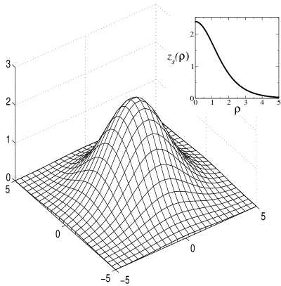
Figure 4: The sketch of the density profile at the saddle point $z_{s}(\bm{\rho})$ corresponding to the solution of Eq. (53) with the boundary conditions (54). The precise radial dependence $z_{s}(\rho)$ obtained by solving Eq. (55) numerically is shown in the inset.

The main exponential dependence of mean switching time $\tau_{i}$ in an infinite sample is given by $e^{F\{z_{s}\}}$. Substituting the numerical result for $z_{s}(\bm{\rho})$ into Eq. (34), one finds paper1

$$\tau_{i}=\tau_{i}^{*}\exp\left[8\zeta\,\frac{\eta a(V_{th}-V)}{\gamma}\right],$$ (56)

where the numerical constant

$$\zeta=\int\!\!d\bm{\rho}\left[\frac{(\nabla z_{s})^{2}}{2}+\frac{z_{s}^{2}}{2}-\frac{z_{s}^{3}}{3}\right]\approx 7.751.$$ (57)

Equation (56) is the counterpart of the result (18) derived for small samples, $S\ll r_{0}^{2}$. Because of the dependence of $r_{0}$ on $V$, see Eqs. (31b) and (14), both types of behavior can be observed in a single device by tuning the bias. At the crossover, $r_{0}^{2}\sim S$, the two results coincide.

The problem of stochastic current switching is similar to the problem of finding the probability of spontaneous decay of a metastable vacuum near a Peierls transition point in ($1+1$) dimensional scalar field theory. The latter problem was solved in Ref. Selivanov, , and the exponential factor in the result for the decay time is analogous to Eq. (56). On the other hand, the prefactor of the decay time is essentially different from $\tau_{i}^{*}$, since we study the shot noise described by classical Fokker-Planck equation, while the false vacuum decay problem is inherently quantum mechanical.

V.1.1 Evaluation of the prefactor

In a finite sample the switching can occur anywhere in the well, hence the prefactor of the switching rate $\tau_{i}^{-1}$ must be proportional to the area $S$. Thus, while $\tau_{i}$ has a large exponential, Eq. (56), its prefactor $\tau_{i}^{*}$ is proportional to $1/S$ and can be small in large samples. Therefore, to fully understand the switching one needs to find $\tau_{i}^{*}$.

The time evolution of distribution function $P\{z,t\}$ in large samples is given by the Fokker-Planck equation (32). To evaluate the prefactor of the mean switching time we again use the expression (36). The procedure is similar to the one for small samples described in Sec. IV.1. However, the integration in Eq. (32) is now over a large sample, and therefore the density at the saddle point becomes non-uniform, Fig. 4. This significantly complicates the evaluation of the prefactor $\tau_{i}^{*}$.

We evaluate both integrals in Eq. (36) in gaussian approximation. As in Sec. IV.1 the integral in the numerator of Eq. (36) is dominated by the minimum of $F\{z\}$ and is given by the expression (41). The denominator of (36) is dominated by the saddle point. Presenting $z(\bm{\rho})$ near the saddle point as $z(\bm{\rho})=z_{s}(\rho)+{\tilde{v}}(\bm{\rho})$, we obtain the expansion of $F\{z\}$ in the form,

$$F\{z_{s}+{\tilde{v}}\}=F\{z_{s}\}+\frac{U_{0}}{2}\!\int\!\!d\bm{\rho}\,{\tilde{v}}(\bm{\rho})[-\nabla_{\rho}^{2}-2z_{s}+1]{\tilde{v}}(\bm{\rho}).$$ (58)

It is convenient to evaluate the integral in Eq. (58) by expanding

$${\tilde{v}}(\bm{\rho})=\sum\limits_{n,m}{\tilde{x}}_{nm}{\tilde{\phi}}_{nm}(\bm{\rho}),$$ (59)

where ${\tilde{\phi}}_{nm}(\bm{\rho})$ are the normalized solutions of the eigenvalue problem

$$[-\nabla_{\rho}^{2}-2z_{s}(\bm{\rho})+1]{\tilde{\phi}}_{nm}(\bm{\rho})={\tilde{\lambda}}_{nm}{\tilde{\phi}}_{nm}(\bm{\rho}).$$ (60)

The boundary conditions for this equation are given by Eq. (54).

Equation (60) can be interpreted as a Schrödinger equation for a particle in the attractive potential $-2z_{s}$ with energy ${\tilde{\lambda}}_{nm}-1$. Since the potential is azimuthally symmetric, we can separate the variables as ${\tilde{\phi}}_{nm}(\bm{\rho})=Q_{nm}(q\rho)\Psi_{m}(\varphi)$. The solutions for the azimuthal part $\Psi_{m}(\varphi)$ are given by $e^{\pm im\varphi}$. Below it will be convenient to use their real combinations, $\cos m\varphi$ and $\sin m\varphi$, and introduce the following notations: $\Psi_{0}(\varphi)=1/\sqrt{2\pi}$, $\Psi_{m}(\varphi)=(\cos m\varphi)/\sqrt{\pi}$ for $m=1,2,\dots$, and $\Psi_{m}(\varphi)=(\sin m\varphi)/\sqrt{\pi}$ for $m=-1,-2,\dots$.

Substituting the expansion (59) into Eq. (58) and using the orthonormality condition for the eigenfunctions, we find

$$F\{\mathbf{{\tilde{x}}}\}=F\{z_{s}\}+\frac{U_{0}}{2}\sum\limits_{n=0}^{\infty}\sum\limits_{m=-\infty}^{\infty}{\tilde{\lambda}}_{nm}{\tilde{x}}_{nm}^{2}.$$ (61)

The discussion leading to Eq. (61) did not rely on the assumption of large sample size. In the case of small samples Eq. (61) reproduces the expansion (42), if one identifies ${\tilde{\lambda}}=\epsilon-1$. This relation is easily understood by noticing that in small samples the density at the saddle point is $z_{s}(\bm{\rho})=1$. Comparing the definition of $\epsilon$ given in the paragraph after Eq. (38) with Eq. (60), where we substitute $z_{s}=1$, we reproduce ${\tilde{\lambda}}=\epsilon-1$.

The form of Eq. (61) suggests that in the case of large samples it is more convenient to evaluate the integral in the denominator of Eq. (36) using variables ${\tilde{x}}_{nm}$ rather than $x_{nm}$. Since the eigenfunctions $\phi_{nm}$ and ${\tilde{\phi}}_{nm}$ are normalized, the expansion coefficients ${\tilde{x}}_{nm}$ are related to coefficients $x_{nm}$ of expansion (38) via an orthogonal transformation. The Jacobian of this transformation equals unity, and therefore the integration over $\prod dx_{nm}$ in the denominator of Eq. (36) can be replaced by the integration over $\prod d{\tilde{x}}_{nm}$.

In order to evaluate the integral in the denominator of Eq. (36) in the $\mathbf{{\tilde{x}}}$-representation, we need to find the eigenvalues ${\tilde{\lambda}}_{nm}$ of Eq. (60). All ${\tilde{\lambda}}_{nm}$ are positive with the exception of one negative eigenvalue, ${\tilde{\lambda}}_{00}<0$, and two zero eigenvalues, ${\tilde{\lambda}}_{0,1}={\tilde{\lambda}}_{0,-1}=0$. Numerical solution of equation (60) yields ${\tilde{\lambda}}_{00}\approx-1.648$. This negative eigenvalue is associated with unstable deviation from $z_{s}$ corresponding to the motion over the saddle point. In Eq. (36) the boundary $\partial\Omega$ of the domain of attraction of the metastable state is orthogonal to ${\tilde{x}}_{00}$-direction, so that the integration in the denominator is performed only over the positive and zero modes. Since each positive ${\tilde{\lambda}}_{nm}$ corresponds to a Gaussian integral, the integration over them is straightforward. The integration over the zero modes is more challenging; to perform it we first need to understand their physical meaning.

The existence of two zero eigenvalues is due to the translational invariance of the functional $F\{z\}$ with respect to any shift of the center of the switching region in the plane of the quantum well. The two zero eigenvalues correspond to two orthogonal to each other directions in the plane along which such a shift can be performed. Indeed, a small shift $\Delta\bm{\rho}$ of the center of switching region results in the following small change in the saddle point density,

$$z_{s}(\bm{\rho}+\Delta\bm{\rho})-z_{s}(\bm{\rho})=\frac{\partial z_{s}}{\partial\rho_{x}}\Delta\rho_{x}+\frac{\partial z_{s}}{\partial\rho_{y}}\Delta\rho_{y}.$$ (62)

One can check by differentiating Eq. (53) with respect to $\rho_{x,y}$ that the derivatives $\partial z_{s}/\partial\rho_{x,y}$ are solutions of Eq. (60) with ${\tilde{\lambda}}=0$. Furthermore, $\partial z_{s}/\partial\rho_{x}=z^{\prime}_{s}(\rho)\cos\varphi$ and $\partial z_{s}/\partial\rho_{y}=z^{\prime}_{s}(\rho)\sin\varphi$, so the azimuthal quantum numbers corresponding to zero modes are $m=\pm 1$ in our notations. Thus we conclude that $\partial z_{s}/\partial\rho_{x,y}=c_{0}{\tilde{\phi}}_{0,\pm 1}(\bm{\rho})$, where $c_{0}$ is a constant.

Substituting these expressions for $\partial z_{s}/\partial\rho_{x,y}$ into Eq. (62) and comparing it with the expansion (59), we find that the coefficients corresponding to zero modes are ${\tilde{x}}_{0,\pm 1}=c_{0}\Delta\rho_{x,y}$. Thus the integral over the zero modes ${\tilde{x}}_{0,1}$ and ${\tilde{x}}_{0,-1}$ amounts to the integration over the possible positions of the center of the switching region in the sample,

$$\int\!\!d{\tilde{x}}_{0,1}\int\!\!d{\tilde{x}}_{0,-1}=c_{0}^{2}\int\!d(\Delta\rho_{x})\int\!d(\Delta\rho_{y})=\zeta\frac{S}{r_{0}^{2}}.$$ (63)

Here the constant $c_{0}$ was found using azimuthal symmetry of $z_{s}$ and the fact that the eigenfunctions ${\tilde{\phi}_{nm}}(\bm{\rho})$ are normalized,

$$c_{0}^{2}=\int\!\!\left(\frac{\partial z_{s}}{\partial\rho_{x}}\right)^{2}\,d\bm{\rho}=\frac{1}{2}\int\![\nabla z_{s}(\bm{\rho})]^{2}\,d\bm{\rho}=\zeta.$$ (64)

The relation between the last integral and the constant $\zeta$ defined by Eq. (57) is proven in Appendix E.

To find the denominator of Eq. (36) in the $\mathbf{{\tilde{x}}}$-representation we also need $D_{ij}$ and $\partial f/\partial{\tilde{x}}_{00}$. They can be obtained from the $\mathbf{{\tilde{x}}}$-representation of the Fokker-Planck equation for large samples. Substituting $z(\bm{\rho})=z_{s}(\rho)+{\tilde{v}}(\bm{\rho})$ with ${\tilde{v}}$ in the form (59) into Eq. (32) and using the orthonormality condition for the eigenfunctions ${\tilde{\phi}}_{nm}(\bm{\rho})$, we obtain the Fokker-Planck equation $\dot{P}={\cal L}P$ with

$${\cal L}=b\sqrt{\gamma\alpha}\sum_{n,m}\left[\frac{\partial}{\partial{\tilde{x}}_{nm}}{\tilde{\lambda}}_{nm}{\tilde{x}}_{nm}+\frac{1}{U_{0}}\frac{\partial^{2}}{\partial{\tilde{x}}_{nm}^{2}}\right].$$ (65)

Here we neglected the terms of higher orders in ${\tilde{x}}_{nm}$. One can easily check that the solution of the stationary Fokker-Planck equation ${\cal L}P_{0}=0$ is $P_{0}=e^{-F}$ with $F$ given by the Gaussian approximation (61).

Comparing Eqs. (IV) and (65) we conclude that $D_{ij}=(b\sqrt{\gamma\alpha}/U_{0})\delta_{ij}$. To find $\partial f/\partial{\tilde{x}}_{00}$ we need to solve Eq. (37) with ${\cal L}$ given by (65), that is

$$\left[-{\tilde{\lambda}}_{00}{\tilde{x}}_{00}+\frac{1}{U_{0}}\frac{\partial}{\partial{\tilde{x}}_{00}}\right]\frac{\partial f}{\partial{\tilde{x}}_{00}}=0.$$ (66)

Solving it with the conditions $f=1$ inside the domain $\Omega$ (i.e., at $x_{0}\to-\infty$) and $f=0$ at the domain boundary $x_{00}=0$, we find that at the saddle point $\partial f/\partial{\tilde{x}}_{00}=-(2|{\tilde{\lambda}}_{00}|U_{0}/\pi)^{1/2}$.

Substituting Eq. (41) for the numerator of Eq. (36), and Eqs. (61) and (63) along with the expressions for $D_{ij}$ and $\partial f/\partial{\tilde{x}}_{00}$ into the denominator of Eq. (36) we reproduce the result (56) with the prefactor given by

$$\tau_{i}^{*}\simeq\frac{\pi^{2}}{4\sqrt{|{\tilde{\lambda}}_{00}|}\zeta bS\alpha^{2}}\Upsilon^{\prime\prime\prime},\quad\Upsilon^{\prime\prime\prime}={\prod_{n,m}}^{\prime\prime\prime}\sqrt{\frac{{\tilde{\lambda}}_{nm}}{\lambda_{nm}}}.$$ (67)

Here the product $\Upsilon^{\prime\prime\prime}$ excludes the factors corresponding to the three non-positive eigenvalues ${\tilde{\lambda}}_{nm}$. The coefficients $\lambda_{nm}$ denote the parameters $1+\epsilon_{i}$ used in Sec. IV.1. They coincide with the eigenvalues of the Schrödinger equation (60) in the absence of the attractive potential $-2z_{s}(\rho)$.

To evaluate the infinite product $\Upsilon^{\prime\prime\prime}$ we need to find the continuous spectrum of Eq. (60). The radial part of ${\tilde{\phi}}_{nm}$ oscillates as a function of $\rho$ with the wavevector $q_{n}$. The phase of these oscillations at $\rho\to\infty$ is shifted by $\delta_{m}(q_{n})$ due to the scattering in the attractive potential $-2z_{s}$. The eigenvalues of the continuous spectrum are expressed in terms of these scattering phase shifts as follows

$${\tilde{\lambda}}_{nm}=1+q_{n}^{2}\simeq 1+\left(\frac{\pi n}{R}\right)^{2}\left[1-\frac{\delta_{m}(\pi n/R)}{\pi n}\right]^{2}.$$ (68)

This result is derived for a round sample of dimensionless radius $R\gg 1$; the derivation and the expression for the phase shifts $\delta_{m}$ are given in Appendix F. The expression for the eigenvalues $\lambda_{nm}$ is given by Eq. (68) with $\delta_{m}=0$.

It is convenient to calculate the logarithm of $\Upsilon^{\prime\prime\prime}$, thereby transforming the product over $n$ and $m$ to a sum. Taking the large sample limit, $R\to\infty$, we replace the sum over $n$ by an integral over $q=\pi n/R$. Then expanding the integrand in small parameter $\delta_{m}/n$, we find

$$\ln\Upsilon^{\prime\prime\prime}\simeq-\frac{1}{\pi}\int_{0}^{\infty}\left[\sum\limits_{m=-\infty}^{\infty}\delta_{m}(q)\right]\frac{q\,dq}{1+q^{2}}.$$ (69)

To investigate the convergence of the integral we need to evaluate the sum of the phase shifts at large $q$. This is accomplished with the help of the following “Friedel sum rule”

$$\left.\sum\limits_{m=-\infty}^{\infty}\delta_{m}(q)\right|_{q\to\infty}=2\zeta$$ (70)

proven in Appendix F. The asymptotic behavior (70) of the phase shifts implies that the integral in Eq. (69) diverges logarithmically at $q\to\infty$. This ultraviolet divergence signals that $\Upsilon^{\prime\prime\prime}$ is determined by a large wavevector cutoff or, equivalently, by some short distance scale. An analogous divergence appeared in the prefactor of the mean switching time in small samples, Sec. IV.1. There we have shown that this short distance cutoff is of the order of the mean free path $l$. Following the same recipe, we cut off the integral in Eq. (69) at $q\sim r_{0}/l$, and with logarithmic accuracy find

$$\ln\Upsilon^{\prime\prime\prime}\simeq-\frac{2\zeta}{\pi}\ln\left(\frac{r_{0}}{l}\right).$$ (71)

Substituting this result into Eq. (67), we obtain the prefactor

$$\tau_{i}^{*}\sim\frac{1}{bS\alpha^{2}}\left(\frac{l}{r_{0}}\right)^{2\zeta/\pi}.$$ (72)

This expression completely describes the parametric dependence of the prefactor of the mean switching time in large samples. On the other hand, because of the ultraviolet divergence of $\Upsilon^{\prime\prime\prime}$, the numerical coefficient in $\tau_{i}^{*}$ cannot be determined without detailed treatment of charge transport at short length scales. 

V.1.2 Renormalization of threshold voltage in large samples

Expression (72) for the prefactor $\tau_{i}^{*}$ implies that in large samples the switching rate $\tau_{i}^{-1}$ diverges at $l\to 0$. In Sec. IV.1.2 we encountered the same problem while considering small samples. There it was shown that the dependence of $\tau$ on the mean free path can be absorbed into the definition of the threshold voltage $V_{th}$. Following the same renormalization technique, one can shift the threshold voltage $V_{th}$ by the amount

$$\delta V_{th}=-\frac{1}{4\pi}\frac{\gamma}{a\eta}\ln\frac{r_{0}}{l},$$ (73)

chosen in such a way that the resulting correction to the exponential in Eq. (56) cancels $\Upsilon^{\prime\prime\prime}$ in the prefactor $\tau_{i}^{*}$, see Eqs. (67), (71). The renormalized result for the mean switching time then takes the form

$$\tau_{i}\sim\frac{1}{bS\alpha_{R}^{2}}\exp\left[\frac{8\zeta\eta\alpha_{R}}{\gamma}\right],\quad\alpha_{R}=\alpha+a\delta V_{th}.$$ (74)

This expression is equivalent to Eqs. (56), (72) up to the correction in the prefactor $\tau_{i}$ due to the substitution $\alpha\to\alpha_{R}$.

The characteristic length scale $r_{0}$ is sensitive to the position of the threshold voltage, so its value has to be renormalized. Since the size of the critical nucleus and $\delta V_{th}$ are coupled to each other, Eq. (73), they should be evaluated self-consistently:

$$r_{R} = \frac{\sqrt{\eta}}{[(\alpha+a\delta V_{th})\gamma]^{1/4}},$$ (75a)

$$\delta V_{th} = -\frac{1}{4\pi}\frac{\gamma}{a\eta}\ln\frac{r_{R}}{l}.$$ (75b)

To find $\delta V_{th}$ one can solve the system of equations (75) iteratively starting with $r_{R}=r_{0}$. The result (73) then should be understood as the first iteration of Eq. (75b).

Upon the substitution of the shift (75b) into Eq. (74), the logarithm of the switching time $\tau_{i}$ acquires an additional logarithmic dependence on voltage due to the bias-dependent renormalization of $V_{th}$. This dependence is physically meaningful and can, in principle, be tested experimentally. However, these corrections to the voltage dependence (56) of $\tau_{i}$ are small, and to the leading order $\ln\tau_{i}$ is still linear in voltage.

V.2 Nucleation near sample boundaries

In Sec. V.1 we studied the nucleation processes in very large samples assuming that the switching initiates far from the boundaries (i.e., at distances significantly greater than $r_{0}$). In this section we show that the switching can be more effective when it is initiated near the boundaries of the sample and evaluate the mean switching time for such processes.

V.2.1 Nucleation at a smooth edge

To study the nucleation near an edge which is smooth on the scale $r_{0}$, we model the sample by a half-plane and set up the coordinate system so that $\rho_{x}$ is the coordinate along the boundary and $\rho_{y}$ is positive inside the half-plane. Then the boundary condition (54) takes the form $z^{\prime}_{\rho_{y}}(\rho_{x},+0)=0$. If we place the center of the saddle-point solution $z_{s}$ shown in Fig. 4 on the edge of the sample, the resulting function

$$z_{e}(\rho_{x},\rho_{y})=z_{s}([(\rho_{x}-\rho_{x}^{(0)})^{2}+\rho_{y}^{2}]^{1/2})$$ (76)

automatically satisfies not only equation (53) but also the boundary condition. Therefore, the expression (76) gives the saddle point density for the half-plane.

One can argue that there are no other saddle point solutions for edge switching. Indeed, suppose that we have a solution ${\tilde{z}}(\rho_{x},\rho_{y})$ of Eq. (53) for a half-plane. Then we can define function $z(\rho_{x},\rho_{y})$ in the entire plane, so that $z={\tilde{z}}(\rho_{x},\rho_{y})$ for $\rho_{y}>0$, and $z={\tilde{z}}(\rho_{x},-\rho_{y})$ for $\rho_{y}<0$. By construction $z(\rho_{x},\rho_{y})$ satisfies Eq. (53) at $\rho_{y}\neq 0$. However, this procedure does not guarantee that the derivative $z^{\prime}_{\rho_{y}}$ is continuous at $\rho_{y}=0$; as a result $\partial^{2}z/\partial\rho_{y}^{2}$ may have a delta-function contribution. More specifically, $z(\rho_{x},\rho_{y})$ satisfies the equation

$$-\nabla^{2}z+z-z^{2}=-2{\tilde{z}}^{\prime}_{\rho_{y}}(\rho_{x},+0)\delta(\rho_{y}).$$ (77)

If in addition ${\tilde{z}}(\rho_{x},\rho_{y})$ satisfies the boundary condition (54), i.e., ${\tilde{z}}^{\prime}_{\rho_{y}}(\rho_{x},+0)=0$, equation (77) coincides with Eq. (53) everywhere in the plane. Then by construction $z(\rho_{x},\rho_{y})=z_{s}(\rho)$, and therefore ${\tilde{z}}(\rho_{x},\rho_{y})$ is given by a half of the saddle-point solution $z_{s}$ shown in Fig. 4 with its center on the boundary of the half-plane. Thus, there are no saddle point solutions for edge switching except (76).

The main exponential dependence of the mean switching time $\tau$ is given by $e^{F\{z_{s}\}}$. In the definition (34) of $F\{z\}$ the integral is taken over the area of the sample. In the case of switching far from the boundaries it is over an entire plane, while for the edge switching this integral is over a half-plane. Therefore $F$ is reduced by a factor of $2$ compared to the case of switching far from the boundaries. Thus, instead of Eq. (56), the expression for $\tau$ at the edge takes the form

$$\tau_{e}=\tau_{e}^{*}\exp\left[4\zeta\,\frac{\eta a(V_{th}-V)}{\gamma}\right].$$ (78)

The evaluation of the prefactor $\tau_{e}^{*}$ is similar to the one for the switching in the middle of a large sample, Sec. V.1.1. In that case we found two types of modes for the azimuthal part of the eigenfunctions ${\tilde{\phi}}_{nm}(\bm{\rho})$ of Eq. (60), namely, $\sin m\varphi$ and $\cos m\varphi$. At the edge only the eigenfunctions proportional to $\cos m\varphi$ are consistent with the boundary condition $z^{\prime}_{\rho_{y}}(\rho_{x},+0)=0$ on the dimensionless density $z$. In the notations of Sec. V.1.1 these modes correspond to $m=0,1,2,\dots$.

The functional $F\{z\}$ is invariant with respect to the shifts of density $z(\rho_{x},\rho_{y})$ along the edge of the sample. Thus $F\{z\}$ has a single zero mode ${\tilde{x}}_{01}$; it corresponds to the eigenfunction with the azimuthal part $\cos\varphi$. Integration over the zero mode, in analogy with Eq. (63), is performed as

$$\int d{\tilde{x}}_{01}=\sqrt{\frac{\zeta}{2}}\frac{{\mathcal{P}}}{r_{0}},$$ (79)

where ${\mathcal{P}}$ is the perimeter of the sample.

To evaluate the prefactor we again use formula (36). Expression (41) for the numerator and the formulas for $D_{ij}$ and $\partial f/\partial{\tilde{x}}_{00}$ in large samples are still applicable, as they were obtained in a way independent of the exact form of the saddle-point density. Following the procedure of Sec. V.1.1, we find the prefactor $\tau_{e}^{*}$ in the form

$$\tau_{e}^{*}=\frac{\pi^{3/2}\Upsilon^{\prime\prime}}{\sqrt{2\zeta|{\tilde{\lambda}}_{00}|}b\gamma^{1/4}\alpha^{5/4}{\mathcal{P}}},\quad\Upsilon^{\prime\prime}=\mathop{{\prod}^{\prime\prime}}_{n,m\geq 0}\sqrt{\frac{{\tilde{\lambda}}_{nm}}{\lambda_{nm}}},$$ (80)

c.f. Eq. (67). The definition of $\Upsilon^{\prime\prime}$ assumes that the factors corresponding to the two lowest eigenvalues, ${\tilde{\lambda}}_{00}$ and ${\tilde{\lambda}}_{01}$, are excluded.

In the product $\Upsilon^{\prime\prime}$ the quantum number $m$ changes from $0$ to $\infty$, while in $\Upsilon^{\prime\prime\prime}$ the same product is from $-\infty$ to $\infty$. Thus using the fact that ${\tilde{\lambda}_{nm}}$ and $\lambda_{nm}$ are even functions of $m$, we obtain

$$\ln\Upsilon^{\prime\prime}\simeq\frac{1}{2}\ln\Upsilon^{\prime\prime\prime}\simeq-\frac{\zeta}{\pi}\ln\left(\frac{r_{0}}{l}\right),$$ (81)

see Eq. (71).

Similarly to Eq. (72) we find the prefactor of $\tau$ for the edge switching

$$\tau_{e}^{*}\sim\frac{1}{b{\mathcal{P}}\gamma^{1/4}\alpha^{5/4}}\left(\frac{l}{r_{0}}\right)^{\zeta/\pi}.$$ (82)

Note that due to the ultraviolet divergence of $\Upsilon^{\prime\prime}$ we can evaluate $\tau_{e}^{*}$ only up to an undetermined constant.

Performing the same renormalization (73) of the threshold voltage as in Sec. V.1.2, one can eliminate the explicit dependence $l^{\zeta/\pi}$ of the prefactor on the mean free path and obtain the following expression for the mean switching time at the edge

$$\tau_{e}\sim\frac{1}{b{\mathcal{P}}\gamma^{1/4}\alpha_{R}^{5/4}}\exp\left[\frac{4\zeta\eta\alpha_{R}}{\gamma}\right].$$ (83)

The exponent in Eq. (83) is factor of 2 smaller than the exponent of $\tau$ for the switching far from the boundaries, Eq. (74). Far from the threshold the exponential factor is dominant, and therefore edge switching is more efficient. To determine which switching mechanism is more efficient near the threshold, one needs to take into account the dependences of the prefactors in Eqs. (74) and (83) on the dimensions of the device.

V.2.2 Nucleation in a corner

In Sec. V.2.1 we considered the processes of switching initiated near a smooth edge of the sample. In samples with pronounced corners, such as the devices of square or triangular shape, there is also a possibility of nucleation in a corner. As we will show, such processes may be more efficient than the nucleation in the interior and at the edges of the sample.

We consider a corner of angle $\theta<\pi$. Similarly to the discussion in the beginning of Sec. V.2.1, one can show that the saddle-point solution $z_{s}(\bm{\rho})$ centered at the corner both solves the equation (53) and satisfies the boundary condition (54).

The subsequent consideration is similar to the one for the switching at a smooth edge of a large sample, Sec. V.2.1. At $\theta<\pi$ the functional $F\{z\}$ does not possess translational symmetry with respect to the shifts of $z(\bm{\rho})$, and therefore there are no zero modes. Due to the boundary condition (54) the allowed modes of the azimuthal part of the eigenfunction ${\tilde{\phi}}_{nm}(\bm{\rho})$ of Eq. (60) are $\cos(\pi m\varphi/\theta)$. Then instead of Eqs. (78) and (80), we obtain

$$\tau_{c}=\frac{2\pi\Upsilon^{\prime}}{\sqrt{|{\tilde{\lambda}}_{00}|}b\sqrt{\gamma\alpha}}\exp\left[\frac{4\theta\zeta\eta\alpha}{\pi\gamma}\right],\quad\Upsilon^{\prime}=\mathop{{\prod}^{\prime}}_{n,m\geq 0}\sqrt{\frac{{\tilde{\lambda}}_{nm}}{\lambda_{nm}}}.$$ (84)

Here ${\tilde{\lambda}}_{nm}$ are the eigenvalues of Eq. (60) with the boundary conditions (54), which take the form $(\partial{\tilde{\phi}}_{nm}/\partial\varphi)|_{\varphi=0,\theta}=0$ for the corner switching. Unlike in Secs. V.1.1 and V.2.1, here at $n\gg 1$ the eigenvalues ${\tilde{\lambda}}_{nm}$ are given by Eqs. (68), (119) with $m$ replaced by $\pi m/\theta$. The product $\Upsilon^{\prime}$ excludes the factor corresponding to the negative eigenvalue ${\tilde{\lambda}}_{00}$.

Following closely the calculations of Secs. V.1.1 and V.2.1, one can find the prefactor of $\tau_{c}$, and the expression for the mean switching time takes the form

$$\tau_{c}\sim\frac{1}{b\sqrt{\gamma\alpha}}\left(\frac{l}{r_{0}}\right)^{\theta\zeta/\pi^{2}}\exp\left[\frac{4\theta\zeta\eta\alpha}{\pi\gamma}\right].$$ (85)

One might expect that at $\theta\to\pi$ this result should coincide with Eqs. (78), (82) describing the edge switching. On the other hand, the prefactors for the edge and corner switching are qualitatively different, since the latter does not depend on the perimeter ${\mathcal{P}}$. This is due to the fact that at $\theta<\pi$ there is no zero mode, i.e., all ${\tilde{\lambda}}_{nm}$ except ${\tilde{\lambda}}_{00}$ are positive. At $\theta\to\pi$ the eigenvalue ${\tilde{\lambda}}_{01}\to 0$, which corresponds to the appearance of a zero mode. In this case one needs to apply the same procedure as in Sec. V.2.1, which will lead to the result (82) for the prefactor.

Performing the same renormalization (73) of $V_{th}$ as in Secs. V.1.2 and V.2.1, we find the expression for the mean switching time at a corner of angle $\theta$

$$\tau_{c}\sim\frac{1}{b\sqrt{\gamma\alpha_{R}}}\exp\left[\frac{4\theta\zeta\eta\alpha_{R}}{\pi\gamma}\right].$$ (86)

Note that at $\theta<\pi$ the exponent of $\tau$ for the corner switching is smaller than that for both interior and edge switching. This makes corner switching more efficient far from the threshold.

VI Discussion

In preceding sections we studied the mean time $\tau$ of switching from the metastable to the stable current state in double-barrier resonant-tunneling structures. We calculated both the exponentials and prefactors of $\tau$ for switching in the small sample regime [Eq. (18)] and for the interior, edge, and corner switching in the large sample regime [Eqs. (74), (83), and (86), respectively]. In this section we discuss the dependence of the mean switching time on voltage for different structural parameters of DBRTS.

We concentrate on the case of round samples, such as the ones used in the recent experiments.Grahn98 ; Teitsworth As we have shown, when the voltage $V$ is tuned close to the threshold, the size of critical nucleus $r_{0}$ is large compared to the radius of the sample $L$, and the device is in the small sample regime. If the voltage is far from $V_{th}$, the device is in the large sample regime, $L\gg r_{0}$. In a typical experiment $\tau$ is measured in a single device for different values of bias. We will therefore assume that all structural parameters and the size of the sample are fixed, and discuss the switching time as a function of voltage. For comparison with experiment we will not distinguish between $r_{R}$ and $r_{0}$ in this section, since the logarithmic in voltage corrections due to the renormalization of the threshold voltage $V_{th}$ are more challenging to observe.

Our approach is valid as long as the exponents in the expressions for the switching time, Eqs. (18), (56), and (78) are much greater than unity. To check when these conditions are satisfied, it is convenient to write the exponent in Eq. (56) as

$$\frac{8\zeta\eta\alpha}{\gamma}=\left(\frac{d}{r_{0}}\right)^{4}.$$ (87)

Here we introduced a new characteristic length scale

$$d\equiv\left(\frac{8\zeta\eta^{3}}{\gamma^{2}}\right)^{1/4}$$ (88)

and applied the definition of $r_{0}$ given by Eq. (31b). Note that the length scale $d$ depends on structural parameters of the device, but not on the sample size or bias.

Similarly, the exponent of the switching time (18) in a small sample can be expressed in terms of $d$ and $r_{0}$ as

$$\frac{4S\alpha^{3/2}}{3\gamma^{1/2}}=\frac{\pi}{6\zeta}\frac{L^{2}}{r_{0}^{2}}\left(\frac{d}{r_{0}}\right)^{4},$$ (89)

where we used the fact that in round samples $S=\pi L^{2}$. This exponent is much greater than unity at $r_{0}\ll(Ld^{2})^{1/3}$. On the other hand, the regime of small sample is defined by the condition $r_{0}\gg L$. Therefore, it exists only in sufficiently small samples, $L\ll d$. In this case close to the threshold there is a region of $3/2$-power law behavior (18). As voltage tuned further away from $V_{th}$ (i.e., at $r_{0}\ll L$), it crosses over to the region of linear voltage dependence of $\ln\tau$ for the regime of large sample, see solid line in Fig. 5a.

In large round samples the mean switching time $\tau$ is given by $\tau^{-1}=\tau_{i}^{-1}+\tau_{e}^{-1}$. Therefore, to find the slope of linear segment of the curve in Fig. 5a, one has to compare the rates of switching in the interior and at the edge. Using Eqs. (74) and (83), the ratio of the rates can be expressed as

$$\frac{\tau_{e}^{-1}}{\tau_{i}^{-1}}\sim\frac{d}{L}\,\exp\left[\frac{1}{2}\left(\frac{d}{r_{0}}\right)^{4}-3\ln\frac{d}{r_{0}}\right].$$ (90)

At $L\ll d$ this result shows that the switching always occurs at the edge rather than in the interior of the sample.

Figure 5: Schematic dependence of the logarithm of the mean switching time $\tau$ on voltage. (a) In round samples at $L\ll d$, close to the threshold there is a region of $3/2$-power law dependence of $\ln\tau$, followed by the region of linear dependence corresponding to the switching at the edge in the regime of large sample. In samples with pronounced corners the region of linear dependence corresponds to the switching at the sharpest corner (dashed line). (b) At $L\gg d$, two regions of different linear behavior corresponding to the switching in the interior and at the edge of large round sample are present. In samples with pronounced corners these two regions are followed by an additional region of linear voltage dependence corresponding to the switching at the corner of smallest angle $\theta$ shown by dashed line. The slope of this linear dependence is smaller by a factor of $\pi/\theta$ than that of edge switching.

To summarize, we found that in samples of radius $L\ll d$ starting at voltage difference $(V_{th}-V)$ corresponding to $r_{0}\sim(Ld^{2})^{1/3}$, one first observes the region of $3/2$-power law dependence (18) of $\ln\tau$. Then, as $(V_{th}-V)$ increases, follows the region of linear dependence (83) corresponding to the switching at the edge in the regime of large sample, see solid line in Fig. 5a.

At $L\gg d$ the system is never in the small sample regime. In this case the dependence of $\ln\tau$ on voltage is linear, but it may be due to either interior or edge switching. According to Eq. (90), at $r_{0}\lesssim d$ and very large $L$ interior switching dominates. At very small $r_{0}$ the exponential in Eq. (90) becomes very large, and therefore the switching takes place at the edge. The crossover voltage $V^{*}$ between these two regions of linear dependence can be determined from the condition $\tau_{e}^{-1}=\tau_{i}^{-1}$ applied to Eq. (90),

$$V^{*}\approx V_{th}-\frac{2\eta^{2}}{\gamma ad^{4}}\ln\frac{L}{d}.$$ (91)

Thus, in these large samples the interior switching (74) dominates between $V^{*}$ and $V_{th}$, whereas at voltage below $V^{*}$ the edge switching (83) prevails. The dependence of $\ln\tau$ on voltage for $L\gg d$ is shown schematically in Fig. 5b by solid line.

If the sample size is of order $d$, the dependence of $\ln\tau$ on voltage can be obtained from the dependences shown in Fig. 5a and Fig. 5b. At $L\sim d$ the region of $3/2$-power law depedence in Fig. 5a and the interior switching region in Fig. 5b disappear. Thus, at $L\sim d$ one can only observe the region of linear voltage dependence corresponding to the edge switching.

In samples with pronounced corners the dependence of $\ln\tau$ on voltage is different due to the possibility of corner switching. The mean switching time $\tau$ in these samples is given by $\tau^{-1}=\tau_{i}^{-1}+\tau_{e}^{-1}+\tau_{c}^{-1}$. At $L\ll d$ an analysis similar to that for round samples shows that the region of linear dependence corresponds to the switching at the sharpest corner, Eq. (86). This dependence is illustrated by dashed line in Fig. 5a. At $L\gg d$, the two regions of interior and edge switching are followed by an additional region corresponding to the switching at the sharpest corner as $(V_{th}-V)$ becomes large, see dashed line in Fig. 5b.

Depending on the ratio of $L$ and $d$ two qualitatively different voltage dependences of $\ln\tau$ are expected. To see whether it is possible to observe them experimentally, we make a crude estimate of the parameter $d$. Substituting $\eta=\sigma/{\tilde{c}}b$ into Eq. (88) and using the estimates of $\gamma$ and $B$ found in Appendix A, we get

$$d\sim\frac{1}{\sqrt{n}}\left(\frac{\hbar\sigma}{e^{2}T_{R}}\right)^{3/4}\left(\frac{T_{L}}{T_{R}}\right)^{1/2}.$$ (92)

To obtain this expression the capacitance of the device per unit area was estimated as $c\sim e^{2}n/E_{F}$, and the energy of the level in the well $E_{0}$ was assumed to be of the order of $E_{F}$. The electron density $n$ in the well is typically of the order of $2\cdot 10^{11}$ $\rm{cm}^{-2}$. The transmission coefficients $T_{L,R}$ of the left and right barriers can be varied in the range from 1 to $10^{-4}$, whereas the conductivity measured in units of $e^{2}/\hbar$ varies from 1 to 100. Assuming $T_{L}\sim T_{R}$, the low bound $d\sim 20$ nm is achieved at $\sigma\sim e^{2}/\hbar$ and $T_{L,R}\sim 1$. The upper bound $d\sim 600$ $\mu$m is achieved by substituting the maximum value of the conductivity and the minimum value of the transmission coefficient. These estimates show that both the cases of $L\ll d$ and $L\gg d$ are experimentally achievable in modern DBRTS, as the sample sizes range from 1 to $10^{3}\mu$m.

The available experimental dataTeitsworth confirm that the dependence of the mean switching time on voltage is indeed exponential. Based on Eq. (92) we estimate $d\sim 10$ $\mu$m, which is somewhat smaller than the radius of the sample $L=60$ $\mu$m. Thus, one should expect the logarithm of the mean switching time to behave as shown in Fig. 5b. (The switching time $\tau$ is referred to as the relocation time in Ref. Teitsworth, .) On the other hand, it was observed in Ref. Teitsworth, that $\ln\tau$ bends upwards, which suggests that $L\ll d$, see Fig. 5a. One of the possible explanations can be that this experiment was performed in superlattices, rather than in DBRTS studied in this paper, which makes our estimate of $d$ unreliable. To test our theory in more detail, it would be interesting to carry out similar measurements of $\tau$ in several samples of different size but with the same structural parameters. This will ensure that both dependences depicted schematically in Fig. 5a ($L\ll d$) and Fig. 5b ($L\gg d$) will be observed. In addition, the exponential dependence in Ref. Teitsworth, is not very pronounced, since $\tau$ varies by only one order of magnitude. This suggests that $\tau$ was measured rather close to the threshold, and therefore the data captures only the initial part of either linear dependence for interior switching [Fig. 5b] or 3/2-power law dependence, Fig. 5a. To observe the entire bias dependence shown in Fig. 5a or Fig. 5b, a measurement of $\tau$ in a wider range of voltage is needed.

Appendix A Calculation of coefficients $A$ and $B$ in Eq. (12)

In this appendix we find the functions $A(N)$ and $B(N)$ in Eq. (12) in the vicinity of the threshold. We will assume that the parameter (15) is small, $\lambda\ll 1$. It will be convenient here to consider $A$ and $B$ as functions of the electron density $n$ rather than $N=nS$.

Let us write the expression for $A=J_{L}-J_{R}$ near the threshold. On the upper branch of the $I$-$V$ curve, the level in the well lies within the conduction band in the left lead; from Eq. (9) we obtain $eV/2+e^{2}N/2C+E_{0}>eV$. On the lower branch, the level is below the bottom of the conduction band in the left lead $eV/2+E_{0}<eV$, so that no current can flow through the well and $N=0$. Therefore, in the bistable region

$$eV-\frac{e^{2}N}{2C}<\frac{eV}{2}+E_{0}<eV.$$ (93)

At $\lambda\ll 1$, it follows from Eq. (8) that $e^{2}N/2C$ is small in comparison with $E_{F}$ and $E_{0}$. One can then see from Eq. (93) that $E_{0}\simeq eV/2$, and Eq. (9) results in $e\phi\simeq eV/2$. Then from Eq. (10b) we find $\Gamma_{R}=\sqrt{2}g_{R}E_{0}$. The expression (7) for the rate $J_{L}$ can also be simplified. For $\lambda\ll 1$ and $g_{L}\sim g_{R}$, to first order in $\lambda$ the expression in the square brackets of Eq. (7) is $(Sm/\pi\hbar^{2})E_{F}$. Using Eqs. (5), (7) and (10a) with all the above simplifications, close to the threshold $A=J_{L}-J_{R}$ can be approximated as

$$A(n,V) = \frac{g_{L}}{\hbar}\sqrt{E_{0}\left(E_{0}-\frac{eV}{2}+\frac{e^{2}n}{2c}\right)}\frac{Sm}{\pi\hbar^{2}}E_{F}$$ (94)

$$-\frac{\sqrt{2}g_{R}E_{0}}{\hbar}nS.$$

The density $n$ on the metastable and unstable branches of the $I$-$V$ curve is found by solving the equation $A(n,V)=0$, which reduces to the quadratic equation

$$\left[\frac{e^{2}n}{2c}\right]^{2}-\left(\lambda\frac{g_{L}}{g_{R}}\right)^{2}\frac{E_{F}^{2}}{2E_{0}}\left[\frac{e^{2}n}{2c}\right]$$

$$+\left(\lambda\frac{g_{L}}{g_{R}}\right)^{2}\frac{E_{F}^{2}}{2E_{0}}\left(\frac{eV}{2}-E_{0}\right)=0.$$ (95)

At the threshold the two solutions for $n$ coincide. This condition enables us to find the threshold voltage and density

$$V_{th} = \frac{2E_{0}}{e}\left[1+\frac{\lambda^{2}}{8}\frac{g_{L}^{2}}{g_{R}^{2}}\frac{E_{F}^{2}}{E_{0}^{2}}\right],$$ (96)

$$n_{th} = \frac{\lambda^{2}}{2}\left(\frac{g_{L}}{g_{R}}\right)^{2}\frac{c}{e^{2}}\frac{E_{F}^{2}}{E_{0}}.$$ (97)

Using Eqs. (16), (97) and the fact that near the threshold $\Gamma_{R}=\sqrt{2}g_{R}E_{0}$, we find the value of $B(n)$ at the threshold:

$$B(n_{th})=\sqrt{2}\lambda^{2}\frac{1}{\hbar}\frac{g_{L}^{2}}{g_{R}}\frac{C}{e^{2}}E_{F}^{2}.$$ (98)

Using Eqs. (96), (97) we expand $A(n,V)$ given by Eq. (94) in Taylor series near $(n_{th},V_{th})$ up to the first non-vanishing terms in $n-n_{th}$ and $V-V_{th}$, respectively. At the threshold $A(n)=0$ has only one solution, i.e., the first derivative with respect to $n$ equals to zero, and therefore we need to expand up to the second order in $n$. The result can be presented as

$$A(n) = -\frac{B(n_{th})}{2}\left[-\alpha+\gamma(n-n_{th})^{2}\right],$$ (99a)

$$\alpha = \frac{2}{\lambda^{2}}\left(\frac{g_{R}}{g_{L}}\right)^{2}\frac{E_{0}}{E_{F}^{2}}e(V_{th}-V),$$ (99b)

$$\gamma = \frac{2}{\lambda^{4}}\left(\frac{g_{R}}{g_{L}}\right)^{4}\left(\frac{e^{2}}{c}\right)^{2}\frac{E_{0}^{2}}{E_{F}^{4}}.$$ (99c)

Since $dU/dN=-2A/B$, the coefficients $\alpha$ and $\gamma$ coincide with those used in Eq. (14).

Assuming rectangular potential profile in the well, parameters $g_{L,R}$ can be estimated in terms of the transmission coefficients of the barriers as $g_{L,R}=T_{L,R}/\pi$.

Appendix B Derivation of Eq. (21) from the detailed balance principle

Let us consider two very close to each other points $\textbf{r}_{1}$ and $\textbf{r}_{2}$ in the well. The system is in a local equilibrium, and the electron distributions are given by Fermi functions. We assume electrons to be sufficiently well coupled to the lattice, so that the temperature $T$ is the same everywhere in the quantum well. Then the probabilities of diffusion between these two points are given by

$$W_{\Delta t}(\mathbf{r}_{1},\mathbf{r}_{2};n)=\sum_{ij}W_{ij}f_{i}(1-f_{j})=\sum_{ij}W_{ij}f_{i}f_{j}e^{\frac{\epsilon_{j}-\mu_{2}}{T}},$$ (100)

$$W_{\Delta t}(\mathbf{r}_{2},\mathbf{r}_{1};n)=\sum_{ij}W_{ji}f_{j}(1-f_{i})=\sum_{ij}W_{ji}f_{i}f_{j}e^{\frac{\epsilon_{i}-\mu_{1}}{T}}.$$

Here $i$ and $j$ label the energy levels at positions $\textbf{r}_{1}$ and $\textbf{r}_{2}$, respectively; $f_{i(j)}$ are the Fermi functions, and $W_{ij}$ is the probability of transition from occupied level $i$ to unoccupied level $j$.

In equilibrium the transition rates satisfy the detailed balance condition:

$$W_{ij}e^{-\epsilon_{i}/T}=W_{ji}e^{-\epsilon_{j}/T}.$$ (101)

Our system is away from equilibrium, since the electrochemical potential $\mu(\mathbf{r})$ varies with the electron density $n(\mathbf{r})$. However, expression (101) is still applicable for the relevant electron scattering processes. For example, in the case of elastic scattering by impurities $\epsilon_{i}=\epsilon_{j}$, and $W_{ij}=W_{ji}$ due to time reversal symmetry, so that Eq. (101) holds. Furthermore, one can easily check that for electron-phonon scattering expression (101) is also valid, because the phonons are not sensitive to the change in electrochemical potential.

Strictly speaking in the presence of electron-electron scattering expression (101) is incorrect. If electron during the transition from state $i$ to $j$ scatters off an electron at position $\mathbf{r}^{\prime}_{1}$, the latter moves to position $\mathbf{r}^{\prime}_{2}$. Then one finds an additional factor of $\exp[(\mu^{\prime}_{1}-\mu^{\prime}_{2})/T]$ in the right-hand side of Eq. (101). However, because the electron-electron interaction is screened, the distance $\mathbf{r}^{\prime}_{2}-\mathbf{r}^{\prime}_{1}$ is of the order of the screening length in the well. The change of $\mu$ at such short distances is small compared to the temperature, and thus Eq. (101) is still approximately correct.

Applying expression (101) to Eqs. (100) we obtain Eq. (21). Since during a short time interval $\Delta t$ an electron can only diffuse over a short distance, the above proof is sufficient for the purposes of Sec. III.1.

As an additional remark, let us show that the expression (21) also holds at larger distances. We consider the probability density $W_{t}(\mathbf{r}_{i},\mathbf{r}_{f};n)$ of diffusion from point $\textbf{r}_{i}$ to a relatively distant point $\textbf{r}_{f}$. Let us divide the time interval $t$ into $N$ small intervals $\Delta t=t/N$. Then $W_{t}$ can be represented in terms of $W_{\Delta t}$ in the following way:

$$W_{t}(\textbf{r}_{i},\textbf{r}_{f};n)=\prod\limits_{k=1}^{N}\int\!\!W_{\Delta t}(\textbf{r}_{k},\textbf{r}_{k+1};n)\,d\textbf{r}_{k+1},$$

where $\textbf{r}_{1}=\textbf{r}_{i}$ and $\textbf{r}_{N+1}=\textbf{r}_{f}$. The distances between the points $\mathbf{r}_{k}$ and $\mathbf{r}_{k+1}$ are small, so that the expression (21) is applicable. Since at small distances $\Delta\mu\ll T$, we can expand Eq. (21) up to the linear terms in $\Delta\mu/T$. Using this expansion we can rewrite each integrand in the above expression in terms of $W_{\Delta t}(\textbf{r}_{k+1},\textbf{r}_{k};n)$. Then evaluating the product over $k$ we obtain Eq. (21). This completes the prove.

Appendix C Calculation of constant $G$ in Eq. (24)

In this appendix we find the constant $G$ in Eq. (24) for an arbitrary scattering mechanism. This is accomplished by expressing $G$ in terms of conductivity $\sigma$.

If a small electrochemical potential gradient is applied in the $x$-direction, it gives rise to an electric current

$$J=-L_{y}\sigma\frac{\partial}{\partial x}\left(\frac{\mu}{e}\right),$$ (102)

where $L_{y}$ is the width of the sample.

Let us find the expression for the current along $x$-axis at $x=0$ in terms of the transition probability density $W_{\Delta t}$. It is given by the difference in the number of electrons crossing the line $x=0$ from left to right and in the opposite direction in unit time, namely,

$$J = \frac{e}{\Delta t}\int_{0}^{L_{y}}\!\!dy_{1}\int_{0}^{L_{y}}\!\!dy_{2}\int_{-\infty}^{0}\!\!dx_{1}\int_{0}^{\infty}\!\!dx_{2}$$ (103)

$$\times[W_{\Delta t}({\bf r}_{1},{\bf r}_{2};n)-W_{\Delta t}({\bf r}_{2},{\bf r}_{1};n)].$$

In equilibrium, i.e. at $\partial\mu/\partial x=0$, the expression for the difference of probability densities in the second line of Eq. (103) vanishes. Away from equilibrium it can found by using the “detailed balance” expression (21):

$$W_{\Delta t}({\bf r}_{1},{\bf r}_{2};n)-W_{\Delta t}({\bf r}_{2},{\bf r}_{1};n)\simeq\frac{\mu_{1}-\mu_{2}}{T}W_{\Delta t}({\bf r}_{1},{\bf r}_{2};n).$$

Expanding $\mu_{1}-\mu_{2}\simeq(x_{1}-x_{2})\partial\mu/\partial x$, one can see that the linearized form of Eq. (103) reproduces Eq. (102) with the conductivity given by

$$\sigma = \frac{e^{2}}{L_{y}T\Delta t}\int_{0}^{L_{y}}\!\!dy_{1}\int_{0}^{L_{y}}\!\!dy_{2}\int_{-\infty}^{0}\!\!dx_{1}\int_{0}^{\infty}\!\!dx_{2}$$ (104)

$$\times(x_{2}-x_{1})W_{\Delta t}({\bf r}_{1},{\bf r}_{2};n).$$

It is important to note that this expression is taken in the limit $\partial\mu/\partial x=0$, so that $W_{\Delta t}$ in Eq. (104) is an equilibrium quantity. Therefore $W_{\Delta t}$ depends only on the distance between ${\bf r}_{1}$ and ${\bf r}_{2}$, i.e., $W_{\Delta t}({\bf r}_{1},{\bf r}_{2};n)=W_{\Delta t}(|{\bf r}_{1}-{\bf r}_{2}|;n)$. Then substituting new variables $x=x_{2}-x_{1}$ and $u=(x_{1}+x_{2})/2$ into the integral in Eq. (104), and integrating over $u$, we find

$$\sigma = \frac{e^{2}}{2L_{y}T\Delta t}\int_{0}^{L_{y}}\!\!dy_{1}\int_{0}^{L_{y}}\!\!dy_{2}\int_{-\infty}^{\infty}dx$$

$$\times x^{2}W_{\Delta t}(\sqrt{x^{2}+(y_{1}-y_{2})^{2}};n).$$

Changing the variables to $y=y_{1}-y_{2}$ and $v=(y_{1}+y_{2})/2$, and using the fact that $\int\!\!dv=L_{y}$, we obtain

$$\sigma=\frac{e^{2}}{4T\Delta t}\int\!\!d{\bf r}\,r^{2}W_{\Delta t}(|{\bf r}|;n).$$ (105)

Finally, comparing Eqs. (24) and (105) we find $G=4T\sigma/e^{2}$.

Appendix D Stationary solution of Eq. (28) near the threshold

In this appendix we discuss the stationary solution $P_{s}\{n\}$ of the Fokker-Planck equation (28) near the threshold. At bias near $V_{th}$ function $b(n)$ can be approximated by a constant $b=b(n_{th})$. Then the equation for $P_{s}\{n\}$ takes the form,

$$\left[u^{\prime}(n)+\frac{\delta}{\delta n}-2\eta\nabla^{2}n-T\frac{2\sigma}{e^{2}b}\nabla^{2}\frac{\delta}{\delta n}\right]P_{s}\{n\}=0.$$ (106)

Here $\eta=\sigma/{\tilde{c}}b$ and $2a/b=2A/B=-u^{\prime}(n)$, c.f. Eq. (13).

It is convenient to present $P_{s}\{n\}$ in terms of a functional $F_{s}\{n\}$, such that $P_{s}\{n\}=\exp(-F_{s}\{n\})$. Then Eq. (106) takes the following simple form

$$-\frac{2\sigma T}{e^{2}b}\nabla^{2}y(\textbf{r})+y(\textbf{r})=f(\textbf{r}),$$ (107)

where we introduced $y(\textbf{r})=\delta F_{s}/\delta n$ and $f(\mathbf{r})=u^{\prime}(n)-2\eta\nabla^{2}n$.

Solution of this equation is given by

$$y(\mathbf{r})=\int d\mathbf{r}^{\prime}\,f(\textbf{r}^{\prime})\mathcal{G}(\mathbf{r}-\mathbf{r}^{\prime}),$$ (108)

where $\mathcal{G}$ is presented in terms of the modified Bessel function $K_{0}$ as

$$\mathcal{G}(\mathbf{r})=\frac{1}{2\pi r_{T}^{2}}K_{0}(r/r_{T}),\quad r_{T}=\sqrt{\frac{2\sigma T}{e^{2}b}}.$$ (109)

At low $T$ the characteristic size $r_{T}$ of the Green’s function $\mathcal{G}$ is very small, so that $\mathcal{G}$ can be approximated by a $\delta$-function. Then Eq. (108) greatly simplifies,

$$\frac{\delta}{\delta n}F_{s}\{n\}=u^{\prime}(n(\mathbf{r}))-2\eta\nabla^{2}n(\mathbf{r}).$$ (110)

The solution of this equation reproduces Eq. (III.2).

The exact criterion for validity of Eq. (110) is given by the condition $r_{T}\ll r_{0}$, where $r_{0}$ is the characteristic size of the function $-u^{\prime}(n)+2\eta\nabla^{2}n$, see Eq. (31b). After substitution of the parameters of the problem from Eqs. (99) and (31b) this criterion takes the form:

$$T\ll\lambda^{2}(1+\lambda)\left(\frac{g_{L}}{g_{R}}\right)^{3}\frac{E_{F}^{3}}{E_{0}^{3/2}\sqrt{e(V_{th}-V)}}.$$ (111)

To estimate the right-hand side of (111) we take the parameters $\lambda\sim 1$, $E_{F}\sim E_{0}$, $e(V_{th}-V)\lesssim E_{F}$ and $g_{L}\sim g_{R}$. Then the criterion (111) reduces to $T\ll E_{F}$. Therefore, one can neglect the temperature term in Eq. (28) unless the structure is strongly asymmetrical, so that $g_{L}\ll g_{R}$.

Appendix E Properties of the saddle point solution $z_{s}(\bm{\rho})$

In this appendix we derive several relations between integrals involving $z_{s}(\bm{\rho})$. Our goal is to express the integrals $\int(\nabla z_{s})^{2}\,d\bm{\rho}$ and $\int z_{s}\,d\bm{\rho}$ in terms of $\zeta$ defined by Eq. (57).

Integrating Eq. (53) over the infinite plane and using the fact that $z_{s}(\bm{\rho})$ decays rapidly at large $\rho$, we find

$$\int\!\!z_{s}\,d\bm{\rho}=\int\!\!z_{s}^{2}\,d\bm{\rho}.$$ (112)

To express the integral in Eq. (64) in terms of the constant $\zeta$, we transform it as

$$\int\!\!(\nabla z_{s})^{2}\,d\bm{\rho} = -\int\!\!z_{s}\nabla^{2}z_{s}\,d\bm{\rho}$$ (113)

$$= -\int\!\!z_{s}^{2}\,d\bm{\rho}+\int\!\!z_{s}^{3}\,d\bm{\rho},$$

where we used Eq. (53) to obtain the second line of (113).

To express one of the integrals in the second line of Eq. (113) in terms of the other, we take advantage of the azimuthal symmetry of the saddle point solution. Multiplying Eq. (55) by $\rho^{2}z^{\prime}_{s}$ and integrating over $\rho$, we find

$$\left.\frac{\rho^{2}{z^{\prime}}_{s}^{2}}{2}\right|_{0}^{\infty}+\int_{0}^{\infty}\rho^{2}\frac{d}{d\rho}\left(\frac{z_{s}^{3}}{3}-\frac{z_{s}^{2}}{2}\right)\,d\rho=0.$$

The first term in this equation vanishes, since $z_{s}\propto e^{-\rho}$ at $\rho\to\infty$. The second term can be simplified by integration by parts, resulting in

$$\int\!\!z_{s}^{3}\,d\bm{\rho}=\frac{3}{2}\int\!\!z_{s}^{2}\,d\bm{\rho}.$$ (114)

Using Eqs. (112)–(114) and (57) we find the following expressions for the integrals in Eqs. (64) and (121),

$$\int\!\!(\nabla z_{s})^{2}\,d\bm{\rho}=2\zeta,\qquad\int\!\!z_{s}\,d\bm{\rho}=4\zeta.$$ (115)

Appendix F Solutions of Eq. (60)

In this appendix we find the eigenvalues of continuous spectrum of the Schrödinger equation (60). We consider a round sample of dimensionless radius $R=\sqrt{S/\pi r_{0}^{2}}$ with the critical fluctuation situated in the center. Note that since we are interested in the case of large samples, the size of the critical fluctuation is small compared to the sample size, i.e., $R\gg 1$.

The potential $-2z_{s}(\rho)$ is azimuthally symmetric, so it is convenient to solve equation (60) in polar coordinates. Separating the variables in as ${\tilde{\phi}}_{nm}(\bm{\rho})=Q_{nm}(\rho)\Psi_{m}(\varphi)$, we can write the equation for the radial part as follows

$$\left[-\frac{d^{2}}{d\rho^{2}}-\frac{1}{\rho}\frac{d}{d\rho}+\frac{m^{2}}{\rho^{2}}-2z_{s}(\rho)\right]Q_{nm}(\rho)=q_{nm}^{2}Q_{nm}(\rho),$$ (116)

where $q_{nm}^{2}\equiv{\tilde{\lambda}}_{nm}-1$. This equation is subject to two boundary conditions: $Q_{nm}(\rho)$ is finite at the origin and $Q^{\prime}_{nm}(R)=0$.

Let us first consider an infinite sample. In the absence of the attractive potential $-2z_{s}$, the finite at the origin solutions to Eq. (116) are the Bessel functions of the first kind $J_{m}(q\rho)$. Their asymptotic behavior at $\rho\to\infty$ is

$$J_{m}(q\rho)\simeq\sqrt{\frac{2}{\pi q\rho}}\cos\left[q\rho-\frac{\pi}{2}\left(m+\frac{1}{2}\right)\right].$$ (117)

In the presence of the attractive potential the asymptotic form of the radial part of the eigenfunction modifies as follows

$$Q_{m}(\rho)\simeq\sqrt{\frac{2}{\pi q\rho}}\cos\left[q\rho-\frac{\pi}{2}\left(m+\frac{1}{2}\right)+\delta_{m}(q)\right].$$ (118)

Here $\delta_{m}(q)$ is the scattering phase shift due to the attractive potential.

For our purposes we only need the expression for $\delta_{m}$ at large wavevectors $q$. At $q\gg 1$ the phase shifts $\delta_{m}\ll 1$, and can thus be found in Born approximation,

$$\delta_{m}(q)=\pi\int_{0}^{\infty}\!\!z_{s}(\rho)J_{m}^{2}(q\rho)\rho\,d\rho,$$ (119)

see also Eq. (14) in Ref. MatveevLarkin, . Note that $\delta_{m}$ is indeed small at $q\gg 1$, because $J_{m}^{2}\propto 1/q$.

In a finite sample the wavevectors $q_{nm}$ are quantized. Using the asymptotic form (118) and the boundary condition $Q^{\prime}_{nm}(R)=0$, we find

$$q_{nm}=\frac{\pi}{R}\left({\tilde{n}}-\frac{\delta_{m}(q_{nm})}{\pi}\right),$$ (120)

where ${\tilde{n}}$ is given by $n+1/4$ if $m$ is even, and by $n+3/4$ if $m$ is odd, with $n$ being a nonnegative integer. Then the eigenvalues ${\tilde{\lambda}}_{nm}$ are given by $1+q_{nm}^{2}$. We use this result in Sec. V.1.1 to calculate $\prod_{n}{\tilde{\lambda}}_{nm}$. This product is dominated by the factors with large $q_{nm}$. Therefore in Eq. (68) we approximate ${\tilde{n}}$ by the radial quantum number $n$ and the argument of $\delta_{m}(q_{nm})$ by $\pi n/R$.

In addition, in Sec. V.1.1 we need an expression for the sum of the phase shifts (119) over the azimuthal quantum numbers $m$. In the right-hand side of Eq. (119) only the Bessel functions $J_{m}(q\rho)$ depend on $m$. Since the sum of $J_{m}^{2}(q\rho)$ over $m$ equals unity, Gradshteyn we find

$$\sum_{m=-\infty}^{\infty}\delta_{m}=\pi\int_{0}^{\infty}\!\!z_{s}(\rho)\rho\,d\rho=2\zeta.$$ (121)

We used Eq. (115) to express the above integral in terms of the constant $\zeta$.

This result can also be derived by means of the Friedel sum rule which states that the sum of the phase shifts in the left-hand side of Eq. (121) is given by $\pi N$, where $N$ is the average number of levels in the attractive potential $U=-2z_{s}(\rho)$. Since the two-dimensional density of states $\nu_{2}=1/4\pi$, we find

$$N=\frac{1}{4\pi}\int\!\!2z_{s}(\rho)d\bm{\rho}.$$ (122)

Combining this expression with the Friedel sum rule we reproduce the result (121).

References

- (1) R. Tsu and L. Esaki, Appl. Phys. Lett. 22, 562 (1973).
- (2) V. J. Goldman, D. C. Tsui, and J. E. Cunningham, Phys. Rev. Lett. 58, 1256 (1987).
- (3) E. S. Alves et al., Electron. Lett. 24, 1190 (1988).
- (4) A. Zaslavsky, V. J. Goldman, D. C. Tsui, and J. E. Cunningham, Appl. Phys. Lett. 53, 1408 (1988).
- (5) R. K. Hayden, L. Eaves, M. Henini, D. K. Maude, and J. C. Portal, Phys. Rev. B 49, 10745 (1994).
- (6) J. L. Jimenez, E. E. Mendez, X. Li, and W. I. Wang, Phys. Rev. B 52, R5495 (1995).
- (7) J. Kastrup, H. T. Grahn, K. Ploog, F. Prengel, A. Wacker, and E. Schöll, Appl. Phys. Lett. 65, 1808 (1994).
- (8) J. Kastrup, F. Prengel, H. T. Grahn, K. Ploog, and E. Schöll, Phys. Rev. B 53, 1502 (1996).
- (9) K. J. Luo, H. T. Grahn, and K. H. Ploog, Phys. Rev. B 57, R6838 (1998).
- (10) M. Rogozia, S. W. Teitsworth, H. T. Grahn, and K. H. Ploog, Phys. Rev. B 64, 041308(R) (2001).
- (11) F. W. Sheard and G. A. Toombs, Appl. Phys. Lett. 52, 1228 (1988).
- (12) N. C. Kluksdahl, A. M. Kriman, D. K. Ferry, and C. Ringhofer, Phys. Rev. B 39, 7720 (1989).
- (13) A. Levy Yeyati, F. Flores, and E. V. Anda, Phys. Rev. B 47, 10543 (1993).
- (14) Ya. M. Blanter and M. Büttiker, Phys. Rev. B 59, 10217 (1999).
- (15) O. A. Tretiakov, T. Gramespacher, and K. A. Matveev, Phys. Rev. B 67, 073303 (2003).
- (16) J. Zinn-Justin, Quantum Field Theory and Critical Phenomena (Oxford University Press, New York, 2001), Chap. 37.
- (17) S. Coleman, Aspects of Symmetry (Cambridge University Press, Cambridge, 1985), Chap.7 and references therein.
- (18) R. Landauer, J. Appl. Phys. 33, 2209 (1962).
- (19) N. G. van Kampen, Stochastic Processes in Physics and Chemistry (Elsevier, Amsterdam, 1997) 2nd ed.
- (20) C. W. Gardiner, Handbook of Stochastic Methods for Physics, Chemistry, and the Natural Sciences (Springer-Verlag, Berlin, New York, 1985).
- (21) L. D. Landau and E. M. Lifshitz, Statistical Physics, Part 1 (Butterworth-Heinemann, Oxford, 1980) 3rd ed., Chap. XIV.
- (22) J. Kurkijärvi, Phys. Rev. B 6, 832 (1972).
- (23) R. H. Victora, Phys. Rev. Lett. 63, 457 (1989).
- (24) M. I. Dykman, E. Mori, J. Ross, and P. M. Hunt, J. Chem. Phys. 100, 5735 (1994).
- (25) M. I. Dykman and M. A. Krivoglaz, Physica A 104, 480 (1980).
- (26) M. I. Dykman, B. Golding, J. R. Kruse, L. I. McCann, and D. Ryvkine, cond-mat/0204621.
- (27) M. I. Dykman, B. Golding, and D. Ryvkine, Phys. Rev. Lett. 92, 080602 (2004).
- (28) D. Ryvkine, M. I. Dykman, and B. Golding, Phys. Rev. E 69, 061102 (2004).
- (29) B. J. Matkowsky and Z. Schuss, SIAM J. Appl. Math. 33, 365 (1977).
- (30) P. Hänggi, P. Talkner, and M. Borkovec, Rev. Mod. Phys. 62, 251 (1990), see Eq. (7.46).
- (31) S. Coleman, Phys. Rev. D 15, 2929 (1977), Erratum D 16, 1248 (1977).
- (32) C. G. Callan and S. Coleman, Phys. Rev. D 16, 1762 (1977).
- (33) M. B. Voloshin, False Vacuum Decay (lecture at the International School of Subnuclear Physics, Erice, 1995).
- (34) M. B. Voloshin, I. Yu. Kobzarev, and L. B. Okun’, Yad. Fiz. 20, 1229 (1974) [Sov. J. Nucl. Phys. 20, 644 (1975)].
- (35) K. G. Selivanov, Zh. Eksp. Teor. Fiz. 94, 57-62 (1988) [Sov. Phys. JETP 67, 1548 (1988)].
- (36) K. A. Matveev and A. I. Larkin, Phys. Rev. B 46, 15337 (1992).
- (37) I. S. Gradshteyn and I. M. Ryzhik, Table of Integrals, Series, and Products (Academic Press, New York, 1980).