Modelling traffic flow fluctuations

Abstract

By analyzing empirical time headway distributions of traffic flow, a hypothesis about the underlying stochastic process can be drawn. The results found lead to the assumption that the headways $T_{i}$ of individual vehicles follow a linear stochastic process with multiplicative noise, $\dot{T}_{i}=\alpha(m_{T}-T_{i})+D\,T_{i}\xi$. The resulting stationary distribution has a power-law tail, especially for densities where cars are interacting strongly. Analyzing additionally the headways for accelerating and decelerating cars, the slow-to-start effect proposed as a mechanism for traffic jam stability can be demonstrated explicitly. Finally, the standard deviation of the speed differences between following cars can be used to get a clear characterization of (at least) three different regimes of traffic flow that can be identified in the data. Using the empirical results to enhance a microscopic traffic flow model, it can be demonstrated that such a model describes the fluctuations of traffic flow quite satisfactorily.

I Introduction

Car drivers keep a certain distance to the car ahead, the space headway $g$. It is defined as the distance between the front bumper of the following to the rear bumper of the leading car. Obviously, this distance depends on the speed $v$ of the cars, the bigger the speed, the bigger is the distance. Therefore, it is useful to define the (net) time headway $T$ as the scaled distance:

$$T:=g/v$$ (1)

Very simple traffic flow models assume, that $T$ is constant for a given driver, or even constant for a given ensemble of drivers. Although this is certainly not true, no ”law” has been verified so far for the dependence of $T$ on $v$.

Note, that the headway definition Eq. (1) is slightly different from the one usually used in the literature: there, the time headway $\widetilde{T}$ is defined as the time between two cars which have passed the same detector. In case that the cars do not accelerate, the two definitions coincide, otherwise a correction has to be applied to transform $T$ into the headways that have been measured by those detectors (let $x(t)$ be the distance of the leading car to the detector):

$$T=\frac{g}{v}=\frac{1}{v}\int_{0}^{\widetilde{T}}x(t)dt\approx\frac{v\widetilde{T}+a\widetilde{T}^{2}/2}{v}=\widetilde{T}+\frac{a}{2v}\widetilde{T}^{2}$$

Usually, $a$ is small, so $T\approx\widetilde{T}$ follows, except for small $v$ and large $\widetilde{T}$.

In the following, the distribution of the headways $p(T)$ will be the object to study instead of individual headways. It contains useful information about the interaction between the cars, and it is mostly responsible for the fluctuations observed in traffic flow, even on a macroscopic scale. Consequently, the traffic engineering literature has a long record of different assumptions to describe the empirically observed headway distributions Adams:1936 ; Cowan:1976 ; Luttinen:1992 . Usually, the underlying process is not stated explicitly, except in the case of free flow, where a Poissonian process is assumed. Clearly, three different regimes of traffic can be observed, which have to be discussed separately. For small speeds $v$, corresponding to a jam, the empirical data are not sufficient to draw solid conclusions. For large speeds, corresponding to free flow, the distribution should finally approach a Poissonian distribution since the cars do not interact with each other anymore. The interesting regime is in between, for speeds in the range $10<v<30$ m/s, where cars are interacting heavily.

Usually, variants of the Poisson distribution are being used for describing headway distributions. Two popular examples of this are the shifted exponential function $p(T)\propto\exp((T-T_{0})/m_{T})$, or the Erlang function $p(T)\propto T^{k}\exp(-T/m_{T})$, where $k$ is an integer. Also, the log-normal function $p(T)=\exp(-((\log(T)-m_{T})/\sigma)^{2}/2)/(\sqrt{2\pi}\sigma T)$ had been proposed for the headways.

More appealing from a physical point of view is the enterprize to relate the observed time headway distributions to a one-dimensional electron gas with repelling interactions Krbalek2001 ; Krbalek2003 . The latter idea leads to a so called gamma distribution of the time headways that is given as follows:

$$p(T)=\frac{(T-T_{0})^{\gamma-1}}{\Gamma(\alpha)m_{T}^{\gamma}}\exp\left(-\frac{T-T_{0}}{m_{T}}\right)\quad T>T_{0}$$ (2)

with the parameters $T_{0}$ (minimum headway), $m_{T}$ (where $T_{0}+m_{T}$ is the mean headway), and $\gamma$, the so called shape parameter. (Traffic engineers name this distribution Pearson type III.)

All these approaches yield sensible results when compared to reality. However, they are not completely convincing, which can be seen by the fact that still no common agreement in the ”right” formulation has been emerged. Probably, this is due to a shortage in reliable and statistically meaningful data. Fortunately, this is going to change, and this work has greatly benefitted from the availability of more detailed microscopic data. The analysis presented below allow for an alternative formulation, which will be worked out in the section II and will be implemented in a certain microscopic car-following model in section III. By doing so, conclusions can be drawn about the macroscopic description of traffic flow.

II Microscopic fundamental diagram

The vast majority of all traffic flow data are collected by induction loops at a certain place on the road. Therefore, just three things can be measured directly and easily (if the detectors are double loop detectors): the speed $v_{i}$ of each of the vehicles crossing the detector, the length $l_{i}$ of this vehicle and the time headway $T_{i}$ between this and the preceding car. When using the net headway, the uninteresting dependence on the car-lengths drops out. The plot of the net headways $T_{i}$ as a function of the speeds $v_{i}$, or much better, the corresponding distribution $p(v,T)$, will be called the microscopic fundamental diagram in the following. An example is presented in Fig. 1, where $p(v,T)$ has been drawn for the left lane of the German freeway A3.

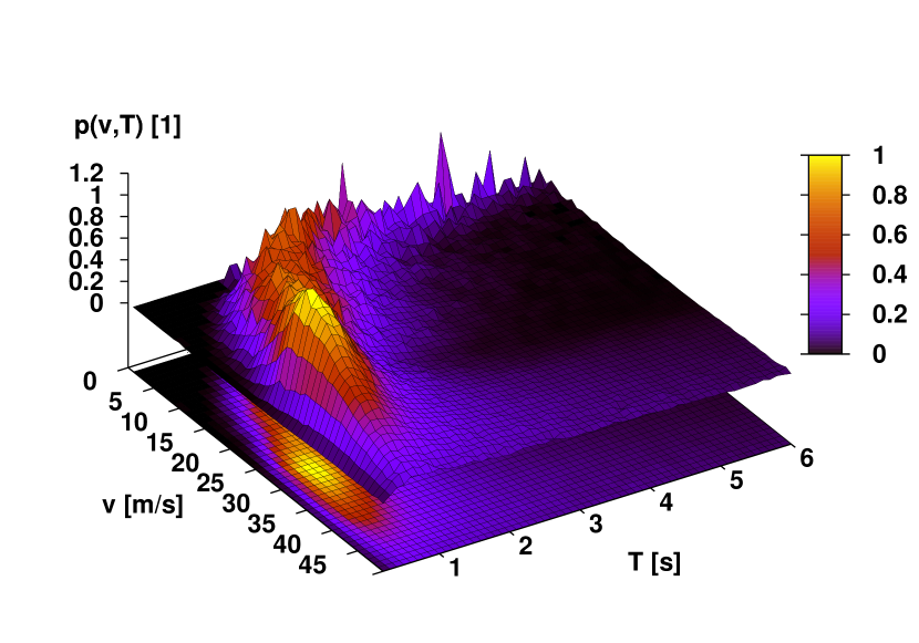
Figure 1: Frequency distribution $p(v,T)$ of the net headways $T$ as function of speed $v$. The raw data are from the left lane of the German autobahn A3 Schad:data:2002 . To determine the net headways, only cars with roughly the same lengthes have been used for this and in the subsequent analysis. This was necessary, since the data contain only the gross headway and the car lengthes.

Three regimes could be identified in Fig. 1. A small speed regime, where the mean headway seems to diverge. An intermediate regime, where the distribution gets relatively small, and finally, the high speed regime where the distribution and the mean headways get fairly large.

The conventional macroscopic fundamental diagram can be obtained from these data by plotting short-time averages of the speed $\langle v\rangle$ versus flow $q$, where the latter is computed as $q=1/\langle T\rangle$ (with $T$ the gross headway). The distribution $p(v,T)$ has a direct relation to the underlying microscopic states of the car-following process, which makes it a very interesting object to study.

II.1 Headway distributions

One cut at constant speed of the distribution in Fig. 1 is drawn in Fig. 2. There, these distribution have been compared to two of the headway distributions above, and one labelled with SDE, which will be derived below:

$$p(T)={\cal N}\left(\frac{1}{T}\right)^{\psi}\exp\left(-(\psi-2)\frac{m_{T}}{T}\right)\quad T\geq 0.$$ (3)

Differently from the other distributions, Eq. (3) has a power-law decay for large headways, with exponent $\psi\approx 4$.

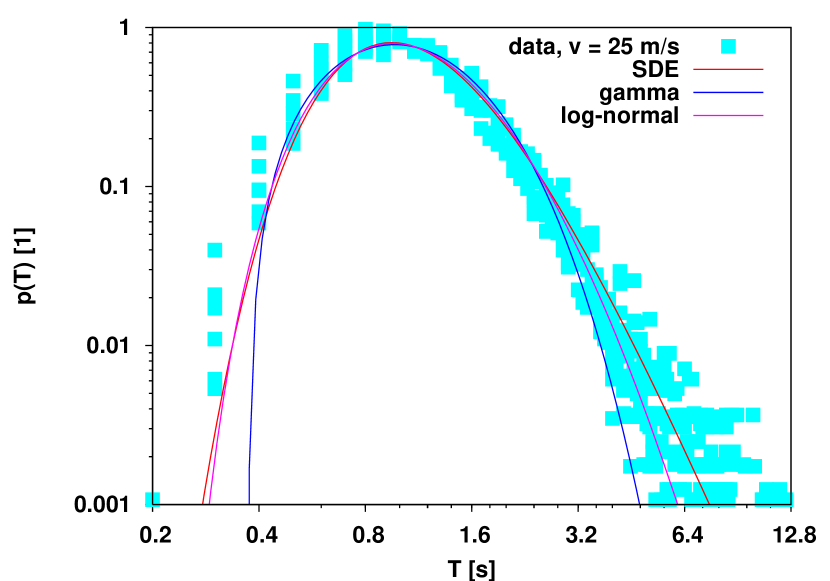
Figure 2: Frequency distribution $p(T)$ of the net headway $T$, left lane, German autobahn A3 Schad:data:2002 , speed $v=25$ m/s. The empirical distribution is compared to a gamma distribution, to a log-normal distribution and to a the distribution Eq. (3). All functions describing the headway distributions have been fitted to the data by a Levenberg-Marquadt algorithm.

As could be seen in the plots, the gamma-distribution is not a bad fit. However, the curve labelled ”SDE” definitely yields the best overlap between data and model. Additionally, this distribution needs just two parameters instead of the three for the gamma-distribution and the log-normal distribution. The curve SDE is the result of assuming that the headway of any particular car-driver unit is controlled by the following stochastic differential equation (SDE)

$$\dot{T}=\alpha(m_{T}(v)-T)+D(v)T\xi,$$ (4)

where $\langle\xi(t)\xi(t^{\prime})\rangle=\delta(t-t^{\prime})$. Here, the constant $\alpha$ is the inverse relaxation time after which the variable $T$ returns to $m_{T}$, and $D$ is the strength of the noise term that disturbs the convergence to $\langle T\rangle$. Both parameters $m_{T}$ and $D$ may depend on the speed $v$ of the cars. The ansatz above is motivated by the idea that a driver has a preferred headway $m_{T}$, which she is not able to realize exactly and instantaneously. This is, because human perception and human reactions are usually rather sloppy. Therefore, a certain time $1/\alpha$ is needed before the preferred headway is reached, and the process is disturbed by a stochastic term which models the uncertainty in human perception and human reaction. It is quite naturally to assume that this uncertainty becomes smaller when the headway itself is smaller, this is modelled by the multiplicative noise term $D\,T\,\xi$. A similar process has been assumed in a completely different context of econophysics. There, it is used to model the pricing of options Hull:1987 .

The stationary solution of the corresponding Fokker-Planck equation to this SDE gives the distribution in Eq. (3), with exponent $\psi=2+2\alpha/D^{2}$ and the normalization constant ${\cal N}$:

$${\cal N}=m_{T}\frac{2^{2\alpha/D^{2}}\left(\langle T\rangle\alpha/D^{2}\right)^{2\alpha/D^{2}}}{\Gamma(2\alpha/D^{2})}$$

(Ito calculus, Stratonovich calculus yields a similar result). As can be seen in Fig. 2, this function yields the best fit, especially for larger headways. Here, the power-law behavior is dominant. Power-laws for different traffic flow variables have been reported in the past (often in simulations of different traffic flow models), see Nagel:Paczuski ; Musha:Higuchi:1976 ; PW:ZfN:1997 ; Ben-Naim:1997 ; Nishinari:2003 for examples. However, they are mostly related to the distribution of the speeds, or the lifetime of traffic jams. Rarely, the headway distributions have been studied.

Therefore, from the analysis of the headway distributions, the hypothesis may be drawn that the preferred headway of a given driver is not a constant but is driven by a simple stochastic process. In the next section, this hypothesis will be discussed again and compared to alternative formulations that can generate the same distribution.

II.2 Correlation times

What cannot be deduced from the freeway data is the correlation times $1/\alpha$ for the headway of a particular car. The headway correlation function between different cars that can be measured from the freeway data is zero, i.e. the headways of different cars are uncorrelated. The autocorrelation function $A(\tau)$ of the headway time-series $T(t)$ of one particular car, however, displays a finite memory. This can be seen in Fig. 3, where $A(\tau)$ for four different cars are presented. They have been computed from data recorded on a Japanese test track Gurusinghe2003 ; pw2003 . There, the trajectories of ten cars following a lead car, all equipped with differential GPS, had been measured. Similar results have been found in other car following data sets as well; however, the decay times are different. A couple of data sets describing car-following processes have been made public, see CDM . Of course, if the autocorrelation function follows a simple exponential delay, namely:

$$A(\tau)\propto\exp(-\alpha\tau),$$ (5)

then the constant $t_{R}=1/\alpha$ is proportional to the relaxation time of the SDE (4). It is not equal to the relaxation time, because the stochastic process driving the headway is filtered through the set of differential equations that describe the car-following dynamics under the assumption that $T$ is constant. The actual result seems to be more complicated, it is consistent with two superposed exponential decay curves $A(\tau)=w\exp(-\tau/\tau_{\text{fast}})+(1-w)\exp(-\tau/\tau_{\text{slow}})$, where the fast decay happens within $\tau_{\text{fast}}=2\ldots 6$ s, while the slower decay took about a factor of ten longer. In general, the $\tau_{i}$ are shorter in dense traffic, for a more detailed analysis the available database is still too narrow.

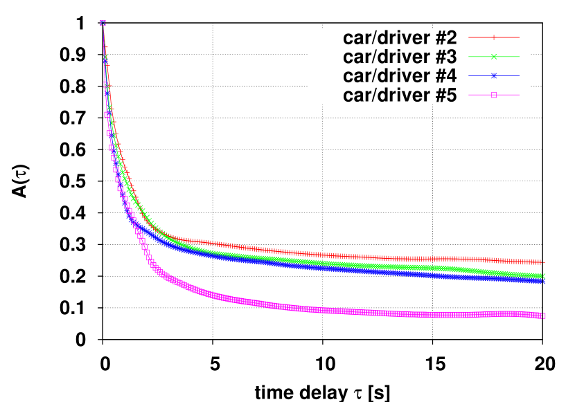
Figure 3: Autocorrelation function $A(\tau)$ for the car-following data, for four different drivers demonstrating individual differences but the same overall behavior.

The two components of the autocorrelation function can be traced back (not shown) to the autocorrelation of the gaps (long-lived component) and of the speed-differences (short-lived), respectively. (Both enter in the computation of $T=g/v$.)

II.3 Dependence on speed

The parameters $m_{T}$ and $D^{2}/\alpha$ may depend on speed, too. For large speeds, $m_{T}$ diverges. This stems from the bigger distances between the freely moving cars. Not as simple to understand is the divergence for the small speeds, later on this will be analyzed more detailed.

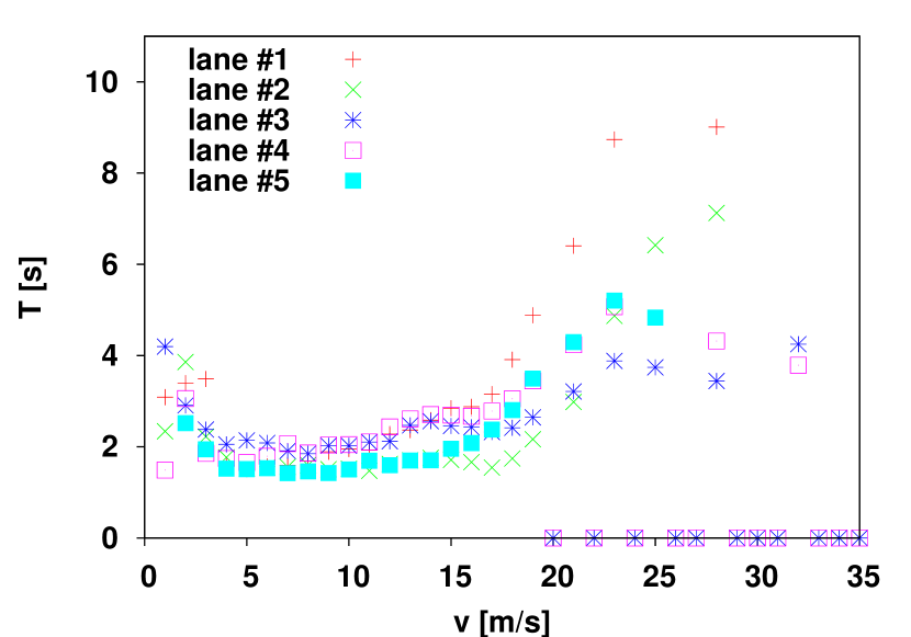
Figure 4: Mean value of headway $T$ as function of the speed $v$. The upper plot is for the German freeway A3, while the lower plot is for the California freeway I-880.

Additionally, there is an intermediate region, where the mean headway depends in a non-trivial manner on the speed of the cars, see Fig. 4. Between two values $v_{1}$ and $v_{2}$ which depend on the circumstances (especially the speed limit), the dependence of $m_{T}$ on speed becomes a decreasing function of speed. This empirical finding has been mentioned already in IDMM . Note, that this is a real effect, since there is no physical reason for the drivers to relax, i.e. to drive with larger headways . On the contrary, anybody would be better off if car-drivers try to keep those short headways, since it would increase the throughput on a highway.

Although the most direct explanation for this dependence of $\langle T\rangle$ on speed $v$ is that of more relaxed driving, an alternative interpretation is possible. Assuming that drivers have different driving attitudes, the increase in headway may be related to a change in the driver population. Borrowing from daganzo:mlane-I ; daganzo:mlane-II the self-explanatory terms rabbits and slugs, it may be assumed that for the smaller speeds more slugs populate the left lane, increasing the mean headway.

Interestingly, this seems to be true only under certain circumstances. It has been found in the data set from the left lane of the German freeway A3, when looking on the other lanes, the dependence is much less clear. Furthermore, drivers on American freeways seem to behave differently. In Banks:2003 it is demonstrated, that the mean headway is independent of speed. An analysis of data measured in the FSP-project (data and description of this project can be found at CDM , too) and from another project on the California freeways I-880 and I-80, respectively, support this result. Using once more the terms rabbits and slugs above, on American freeways the different lanes are more homogeneous, since there is no reason for the slugs to stay on the right lane(s).

That is not all. As can be suspected, the noise strength, too, is a function of speed, with $D^{2}/\alpha$ decreasing as speed decreases. This can be seen in Fig. 5.

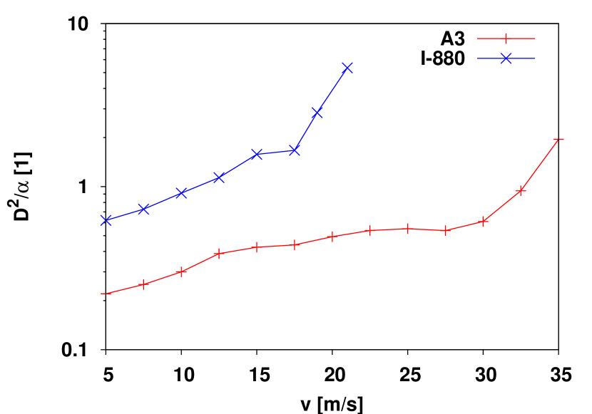
Figure 5: Noise strength $D^{2}/\alpha$ as function of speed $v$. For smaller speeds, the noise is smaller. The numbers for $D^{2}/\alpha$ have been obtained by fitting each $p_{v}(T)$ histogram with a Levenberg Marquadt algorithm. The I-880 site had a speed limit of 55 mph (24.6 m/s), the data are restricted to the rush-hours, so larger speeds than 22 m/s do not contain enough statistical weight to allow for a similar analysis.

While the overall dependence is the same for the US-example as well as for the German A3 data, the width of the headway distribution in the American data is bigger by about a factor of almost three.

II.4 Slow–to–start behavior

While the creation mechanism of jams is still controversial, the fact that jams are stable can be understood much more easily. The simplest idea that causes stable jams is what has been called quite tellingly a slow-to-start mechanism Sch:Sch:slow-to-start . It is assumed, that a car leaving a jam needs considerably more time-headway than what is needed in maximum flow conditions. Already in Newell1962 such a mechanism is proposed, to explain the jam-waves observed in the Holland tunnel in New York. However, the empirical support reported so far is weak. E.g. the model proposed in Newell1962 assumes, that the fundamental diagram in the congested region consists of two branches, one for accelerating and the other one for decelerating traffic. Usually, the scatter in the empirical data is so big, that the two branches are completely hidden by the scatter, if they exist at all (see Fig. 6). Again, the single-car data analyzed here help to explore this putative mechanism in greater detail. This is displayed in Fig. 6. There, the

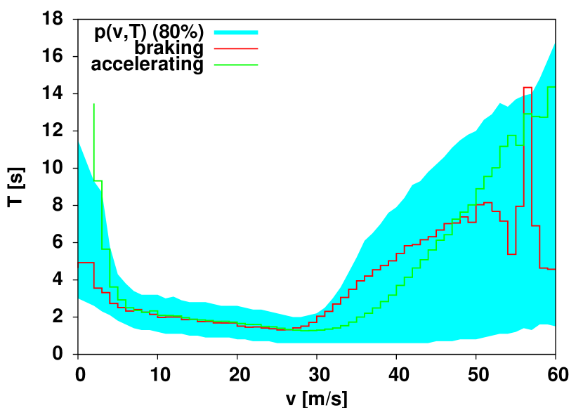
Figure 6: Slow-to-start behavior. Plotted is headway $T$ versus speed $v$. The filled area represents the center 80% of the mass of the frequency distribution $p(v,T)$. The line labelled acceleration is from cars where $v_{i}>v_{i-1}+v_{c}$ holds, while the braking line is from cars with $v_{i}<v_{i-1}-v_{c}$. The threshold $v_{c}$ has been set to $v_{c}=0.5$ m/s.

headway velocity data have been averaged for cars where acceleration or deceleration can be assumed. Since acceleration or deceleration is not measured in these data, it is assumed that a car is accelerating when $v_{i}>v_{i-1}+v_{c}$ holds. Vice versa, if $v_{i}<v_{i-1}-v_{c}$ holds, it is decelerating. Definitely, a more thorough analysis had to wait for trajectory data. Currently, there are a couple of projects running world-wide to collect those data, the one that is probably most advanced is NGSIM-2004 . Nevertheless, two interesting observations can be made already with the single car data available for this study. First, there is indeed a slow-to-start regime for speeds smaller than 5 m/s. By comparing with a simulation where this feature has been explicitly put in (see next section for details), it could be stated that the increase in headway is not restricted to accelerating cars. The simulation data coincide with the empirical data only if the assumption is stated, that for small speeds (below 5 m/s) car drivers increase their time headway considerably.

The second interesting feature in Fig. 6 is that for larger speeds there is a regime where the decelerating cars (instead of the accelerating cars) have the larger time headway. The latter feature is hard to understood right now, it certainly needs more work to explain and is most likely related to multi-lane phenomena.

II.5 Regimes of traffic flow

Figure 6 already demonstrates, that there are different regimes of traffic flow which may be discernable on the basis of the mean headway for accelerating and decelerating cars. The different regimes can be demonstrated more clearly by analyzing the standard deviation of the speed differences between following cars:

$$\Delta^{2}(v)=\frac{1}{N}\sum_{i=1}^{N}(v_{i}-v_{i-1})^{2}-\left(\frac{1}{N}\sum_{i=1}^{N}(v_{i}-v_{i-1})\right)^{2}.$$ (6)

The speed $v$ used for reference on the left hand side of the equation is $v_{i-1}$, i.e. the expression above measures the width of the distribution of speed differences, which in fact depends on the speed itself: for large speeds, corresponding to free flow conditions, speed differences can be fairly large, while they become small under congested conditions (smaller speed).

The function $\Delta(v)$ which is shown in Fig. 7 displays a fairly complicated behavior.

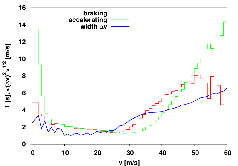
Figure 7: The function $\Delta(v)$ for data from the German freeway A3, together with the headway data determined as in Fig. 6, plotted here for reference.

At least, three different regimes can be separated: a small speed regime, an regime of intermediate speeds where $\Delta_{v}(v)$ is small an roughly constant, and a high-speed regime, where $\Delta_{v}(v)$ increases with speed. What all this means becomes clearer by looking at $\Delta_{v}$ as function of the fundamental diagram. The region with comparably small $\Delta_{v}$ is found in the middle of the fundamental diagram, and this is more or less the region that is usually identified with synchronized flow (see KernerPRE2002 for a good summary of all the previous work on synchronized flow).

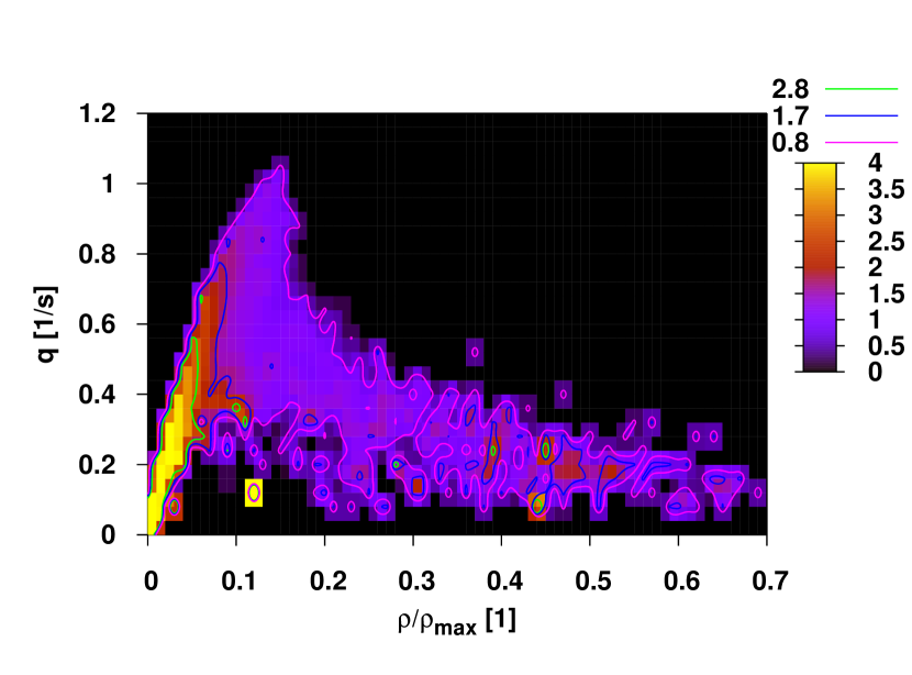
Figure 8: The standard deviation of speed-differences, $\Delta_{v}$, as function of occupancy $\rho/\rho_{\text{max}}$ and flow $q$, again for data from the left lane of the German freeway A3. Note the plateau of constant $\sigma_{v}$ (the contour lines labelled with 0.8 and 1.7 m/s).

This means, that the variable $\Delta_{v}$ as defined above gives a fairly well statistically meaningful characterization of the states of traffic flow, which are associated with synchronized flow. However, it could be stated that the region of small $\Delta_{v}$ extends to the left, into the high-flow regime. The high-flow regime is assumed to be different from the synchronized flow regime, however the Fig. 8 here suggests that even the high flow state is just a synchronized state of traffic flow. To make clear that this is different from the view in KernerPRE2002 , this entire region will be called homogeneous flow of interacting cars in the following.

A similar conclusion has been drawn already in Helbing:block . With respect to the interaction, it is quite naturally to recognize high flow states as similar to the other states where cars are interacting heavily: in both cases, the driving behavior is very concentrated and attentive of the surrounding cars, otherwise those high-flow states could not be sustained.

To summarize, three different regimes of traffic flow may be discerned clearly: the low demand regime, where the headway distribution is Poissonian, the interaction regime where headways are power-law distributed, and a jammed region, where headways probably are something different. The interaction-dominated regime is the one of the small $\Delta_{v}$.

This issue will be discussed once more in the light of the discussion about the model to be described next.

III Consequences

So far, empirical results have been presented. In this section, the consequences for microscopic models will be discussed. For the macroscopic models, similar ideas may be followed.

Before explicitly demonstrating how the empirical results can be implemented into a certain microscopic model of traffic flow, the basic assumption of this work should be discussed more detailed. It has been assumed, that the preferred headway of a driver follows a simple stochastic process defined by Eq. (4). There are (at least) two additional hypotheses that lead to the same or a similar distribution. The first one is to assume that the $T_{i}$ of a driver is constant Cassidy:memory:1998 and that the $T_{i}$ of all the drivers are distributed according to the distribution Eq. (3). The second hypothesis assumes a stochastic process for $T$ without memory. Both hypotheses can be rejected: the first alternative because the empirical data from the car-following experiments demonstrate that $T$ is not constant for a particular driver. The second alternative can be ruled out by comparing simulation results of the model defined next with different stochastic processes for the headway. This results in a headway distribution that is definitely different for the white-noise assumption than it is for a time headway driven by Eq. (4). (This does not rule out that the $m_{T}$ of the drivers are distributed, too.)

III.1 Models

As a simple example, the model introduced in Krauss:Metastable will be extended with the empirical results above. Obviously, these results can be transferred to most of the known models, provided they have something like a preferred distance. While this will lead to the correct headway distribution, the macroscopic behavior of different models might be different. The model Krauss:Metastable , and a very similar model Gipps:following can be derived from a safety condition, namely:

$$d(v_{i})+v_{i}\,T_{i}\leq d(v_{i-1})+g_{i}$$ (7)

where the $d(v_{i})=v_{i}^{2}/(2b)$ are the braking distances of the following (index $i$) and the leading car (index $i-1$), respectively. The deceleration $b$ is understood as a comfortable braking deceleration, not the maximally possible one. The constant $T_{i}$ is the preferred headway of the driver, $g_{i}^{\star}=v_{i}T_{i}$. The equation above can be solved to yield the safe speed:

$$v^{(i)}_{\text{safe}}=-bT_{i}+\sqrt{(bT_{i})^{2}+v_{i-1}^{2}+2bg_{i}}.$$ (8)

From this, the final model in Krauss:Metastable is constructed by assuming an update equation of the form (denoting time as $t$ and the time step size by $h$):

$$v_{i}(t+h)=\min\{v_{i}(t)+a_{i}h,v_{\text{safe}},v_{\text{max}}\},$$

where the constants $a_{\text{max}},v_{\text{max}}$ are parameters (maximum acceleration and maximum speed, respectively) of the model. (The complete model additionally contains a noise term.) However, this equation describes the speeds and not the acceleration, the speed adapts to the safe velocity almost instantaneously (within one time-step $h$). To define an equation for the acceleration, the model can be formulated similar to the optimal velocity models Newell1962 ; Bando:etc:pre :

$$a_{i}=(v^{(i)}_{\text{safe}}-v_{i})/T_{\text{acc}}$$ (9)

This describes the relaxation of the current speed towards the safe speed, with a time constant $T_{\text{acc}}$. This time constant is basically the autocorrelation time of the resulting acceleration time series. Extracting this number from an acceleration time-series typically gives values between one and three seconds for this constant.

Equations (8),(9) define the deterministic part of the model; it does not contain an explicit white noise term that acts on the acceleration. This (white) acceleration noise term that is often used in physical models of traffic flow is clearly unrealistic, and the stochastic process defined in Eq. (4) is an alternative. Together with a discrete version of Eq. (4), the model is fully specified:

$$x_{i}(t+h) = x_{i}(t)+v_{i}(t)\,h$$ (10)

$$v_{i}(t+h) = v_{i}(t)+a_{i}(t)\,h$$ (11)

$$T_{i}(t+h) = T_{i}(t)+\alpha h(m_{T}-T_{i})+$$ (12)

$$\sqrt{h}DT_{i}\xi_{i},$$

with $a_{i}(t)$ as given in Eq. (9). Here, $\xi_{i}(t)$ is a random number in $[-1,1]$. Formally, Gaussian random numbers should be used here. To get a fast implementation, this can be omitted Honerkamp:Book . Of course, to describe freeway traffic realistically, $m_{T}(v)$, $D(v)$, and the parameters needed by the model have to be provided. They can be obtained from the empirical data such as Fig. 4 or by directly fitting this model to traffic flow data, see Brockfeld2003a ; Brockfeld2004a for examples. The numbers found from the freeway data are $\alpha=1/2\ldots 1/5$ s^-1, $D=0.5$, $T_{\text{acc}}=1.0$ s.

The model can be made crash free by enforcing in each update step $v_{i}\leq v_{\text{safe}}$.

A more detailed analysis of this new model will be performed elsewhere. Here, the behavior of the model with respect to the question of the traffic flow phases will be discussed. However, even microscopically the model is in line with two important empirical observations. First, it yields the noisy oscillations in speed-difference headway space, see Fig. 9. Secondly, the time headway distribution is very similar to the empirical headway distributions.

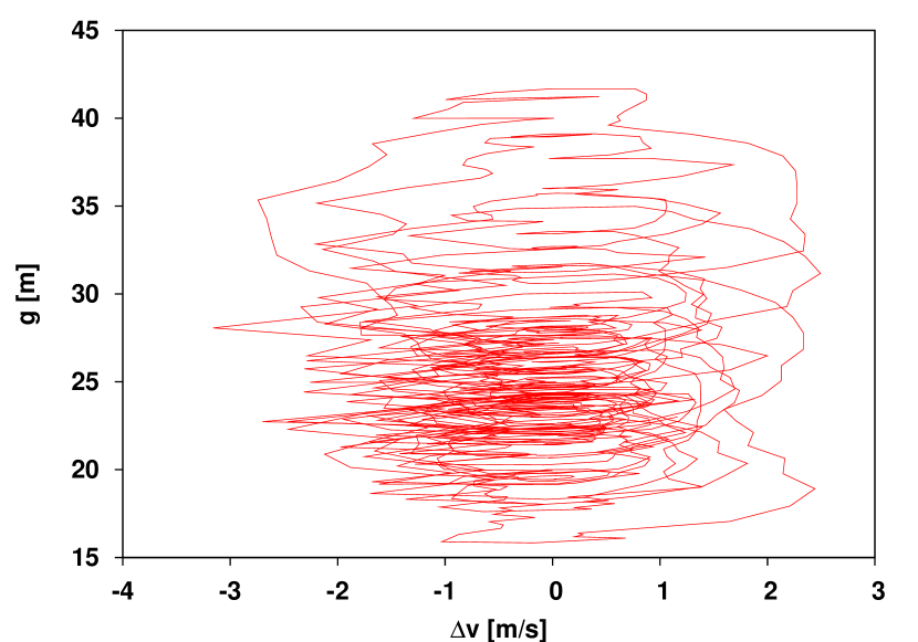
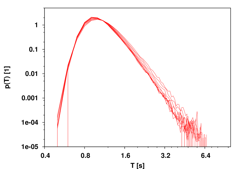
Figure 9: Oscillations in speed difference $\Delta v$, distance $g$ space (above) and the headway distribution (below) for a simulation run with the model defined in Eqs (10) – (12). Parameters are $D=0.5$, $\alpha=1/5$ s^-1, $h=0.4$ s, $m_{T}=1$ s. The driving parameters were set to $a_{\text{max}}=1.5$ m/s², $b=2$ m/s², and $v_{\text{max}}=31$ m/s. A simulation with $n=200$ cars on a closed loop was run for 10000 s before data were sampled for another 10000 s.

III.2 Macroscopic behavior

The model as defined above has only one solution as function of the density: a homogeneous state, with a width in the time headway distribution given by $D^{2}/\alpha$ of the SDE above. This can be seen in the fundamental diagram, see Fig. 10.

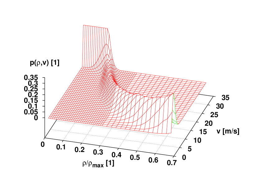
Figure 10: Fundamental diagram of the model Eqs (10) – (12). Parameters and simulation set-up are the same as in Fig. 9.

The mean value $\langle v\rangle$ of this distribution is, of course, a function of density $\rho=1/(g+\ell)$, where $\ell$ is the length of a car, and $\rho_{\text{max}}=1/\ell$ is the maximum density. It can be obtained approximately analytically by setting $a_{i}=0$ in Eq. (9), integrating the resulting expression over the distribution $p(T)$ of and solving for $v(g)$. This yields:

$$\langle v(\rho)\rangle\approx\left\{\begin{array}[]{ll}v_{\text{max}}&\mbox{if}\quad\rho<\rho_{c}\\ \frac{1}{m_{T}}\left(1/\rho-\ell\right)&\mbox{else}\end{array}\right.$$ (13)

This formula fits quite well the simulated fundamental diagram, however a slightly larger value of $m_{T}$ is needed to obtain an exact fit.

However, the model is not complete, because it lacks a mechanism that stabilizes a jam once it is created. As pointed out above, the empirical data analyzed above seem to support the idea of a slow-to-start mechanism. There are different means to implement such a mechanism. The one chosen here is to alter the relation for $v_{\text{safe}}$ by making $v_{\text{safe}}$ smaller for small speeds. This is done in Eq. (7) to arrive at a modified $\tilde{v}_{\text{safe}}$:

$$\tilde{v}^{(i)}_{\text{safe}}=\left\{\begin{array}[]{ll}v_{\text{safe}}-\epsilon(v_{i}-v_{c})&\mbox{if}\quad v<v_{c}\\ v_{\text{safe}}&\mbox{else}\end{array}\right.$$ (14)

Of course, $\tilde{v}_{\text{safe}}>0$ must be demanded explicitly.

This changes the behavior of the model. It becomes bistable in some regions of the control parameter space $\rho,D$. The corresponding phase diagram is displayed in

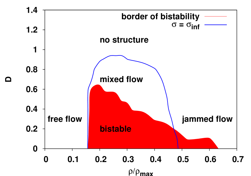
Figure 11: Phase diagram of the model Eqs (10) – (12). Parameters are as in Fig. 9, additionally a slow-to-start mechanism as in Eq.14 has been adopted. Simulation has been run for 40000 s, with 500 cars for each value of $\rho$ and $D$. See text for details on how the separating lines have been obtained.

Fig. 11. To demonstrate bistability, the system has been started either in a jammed state or in a homogeneous state. After running for 40000 s, the probability distributions $p^{\text{hom}}(v)$ and $p^{\text{jam}}(v)$ are being analyzed. For bistable parameter values, there should be a difference between the two distributions, which can be measured by computing $\eta=\int p^{\text{hom}}(v)-p^{\text{jam}}(v)dv$. This is a number between zero and one, with $\eta=0$ indicating equal outcomes of the simulation. The shaded area in the plot above is the area where $\eta>0.1$.

The different areas free flow, jammed flow, mixed flow, and unstructured have been assigned on the basis of the standard deviation of the speed $\sigma(\rho,D)$ which can be computed from $p(v)$, too. The whole approach is very similar to Nagel:breakdown . Let’s start with the unstructured state. When increasing the noise $D$ of the headway distribution, the speed distribution must finally approach the constant distribution in $[0,v_{\text{max}}]$, with standard deviation $\sigma=:\sigma_{\infty}=v_{\text{max}}/\sqrt{12}$. The simulation results confirm this. This state may be called, in analogy with equilibrium thermodynamics, the high temperature state.

For smaller values of $D$, the system can be in three different states: a free flow state, where all cars move with approximately the free speed, the jammed state where all cars move with small speeds near zero, and a mixed state where the system consists of a mixture of freely moving and jammed cars. This picture of nucleation is quite familiar from the theory of (equilibrium) phase transitions. Additionally, the system may be in the homogeneous state, where all cars move with the same speed, which is smaller than the free flow speed. For small $D$, the standard deviation of speed therefore is very small for small densities, since $p(v)$ is close to a delta-function there. The same is true for very large densities. In between, the system may consist of a mixture of jammed and free driving cars, in this case the standard deviation of speed becomes maximal, because $p(v)$ consists of two delta-peaks located at $v=0$ and $v=v_{\text{max}}$, respectively. In this case, $\sigma=v_{\text{max}}/2$. For moderate values of $D$, the peaks are wider, therefore $\sigma$ descreases until it finally reaches $\sigma_{\infty}$.

Therefore, the line where $\sigma=\sigma_{\infty}$ can be used to discern these states, and that is what is drawn in Fig. 11.

The homogeneous state, which does not fit into the picture borrowed from thermodynamics, is stable only for small $\rho$ and small $D$, for larger values it decays. With respect to phenomenology of traffic flow, it is important that there is a region in this phase diagram the homogeneous state co-exist with the mixed state, at least to the time resolution applied here (each simulation for each of the data-points $\rho,D$ has been run for 40000 s). What happens depends on the initial conditions, or, in the case of an open system, on the boundary conditions applied. Such a bistability is a very attractive feature, since it gives an idea why different states of traffic may be observed in cases where anything else is identical. This gets additional back-up with the observation, that the empirical data leads to a value of $D=0.5$, which is in the bistable region (depending, of course, on $\rho$).

III.3 Comparison with empirical data

The model compares qualitatively very well with real data. However, it is still not a good model in the sense of comparing well even quantitatively with empirical traffic flow data. However, on the level of macroscopic measures like the headway distribution $p(v,T)$, the comparison is quite successful, as Fig. 12 demonstrates.

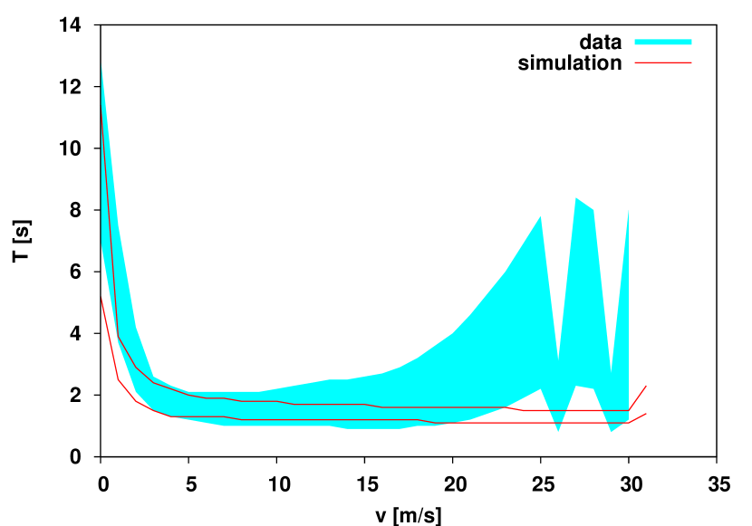
Figure 12: The 25th-percentile and the 75th-percentile lines of the empirical probability distribution $p(v,T)$ compared to simulation data. For the simulation, the same set-up as in Fig. 9 has been adopted. The simulation data are from a scan of the fundamental diagram, i.e. a simulation has been run for different densities.

There, the microscopic fundamental diagram has been compared with the empirical one. Although such comparisons are of limited value, it demonstrates that at least the fluctuations of traffic flow are well described by the model introduced here.

To make this comparison more quantitative, new features must added. These include, but are not restricted to, good ideas how crash-freeness is achieved by human drivers, anticipation to the behavior of other cars in front, more details on how the acceleration is chosen by a driver, issues related to driver inhomogeneity, and multi-lane modelling, see pw2003 for more details.

IV Conclusions

IV.1 Synchronized flow

As discussed already in section II.5, the states of traffic flow where the interaction between the cars is important have a relation to the synchronized traffic flow. We will not enter the discussion about the truly complicated phenomenology of synchronized flow, see KernerPRE2002 for details on that. However, a synthesis is tried that unifies the simulation results with the empirical results, and further more, may bring together the different views about synchronized flow put forward so far (see KernerPRE2002 ; daganzo:critique:sync ; SchreckiPRL2004 ).

The idea here, which is motivated by the surprising stability of the homogeneous flow of the traffic flow model above (and in fact of most traffic flow models, to make them truly unstable is not a simple task), is as follows. There is a large region of traffic flow states where the homogeneous state as function of density is stable. Definitely, homogeneous does not mean that the relevant variables like flow, density, and speed are distributed sharply. In fact, this work here is about a clean description of the fluctuations in the headways of the cars, so homogeneous means a distribution of a certain width. Only for very large densities, or for truly strong external perturbations, there is in fact an instability where breakdowns could occur. These breakdowns are probably related to the pinch effect described in KernerPRE2002 .

So, when such a system is regarded on a closed loop (no boundary effects are present), just three different states might be possible: a free flow state with a Poissonian headway distribution, a homogeneous state with a power-law headway distribution, and a jammed region. In a certain range of densities and noise amplitudes $D$ the jammed state and the homogeneous state are both stable, i.e. different initial conditions lead to different final states. Whether or not there is a phase transition in the sense of non-equilibrium physics between these different states is right know not clear. Even if the system manages to stay at the homogeneous state while increasing the density, there is a transition where the Poissonian distribution is translated into the power law distribution. Although there is a really nice symmetry between these two states (the gamma distribution for $T$ transforms into the power-law distribution under the transformation $T\to 1/T$), it is not clear whether this is in fact a phase transition. But even if it is, it is one of second or even higher order, because nothing jumps here: it is simply the number of cars that drive freely which is reduced until finally all cars are following its lead car, without any chance to overtake.

In the case of an open system, more can happen. Any capacity drop downstream caused by an incident, or a change of inflow at an on-ramp, causes what have been called the back-of-the-queue states, and the transition from apparently free flow into this state is a discontinuous, first order phase transition. (Speed jumps from a large to an intermediate value.) This congested state with reduced speed is exactly what has been called homogeneous flow of interacting cars above. In fact, some of the data analyzed in this contribution (data from the I-80 in California) are from a site where a toll station exists downstream which causes the daily break-down in this area.

This is in line with theoretical considerations about very simple open traffic flow systems. There, it could be demonstrated explicitly, that the transition from a free flow state to the congested flow dominated by the capacity constraints downstream, is in fact a first-order transition Schuetz1999 ; SchuetzInDomb ; Cheybani:2001a ; Cheybani:2001b ; Helbing:5phases ; Namazi2002 ; Rajewsky ; Appert2001 . So, what may look like a first order transition of the bulk system might in fact be a transition caused by the boundary.

IV.2 More general remarks

There is one final question to be answered: why is the headway driven by such a process? Part of the answer might be what has been proposed recently as the human driver model Helbing:HDM . There, it is assumed that a driver is simply not capable of estimating the distance and the speed difference to the car in front timely and accurately. This is certainly true, and the autocorrelation results presented in this paper lend empirical support to such an idea. However, it introduces two things that are truly hard to measure: how wrong do humans estimate these two numbers, and how do they modify their outdated measurements. It should be simple to demonstrate, that in the context of the model above, this assumption leads to a similar result for the time headway distribution, however, preliminary simulation results demonstrate that the resulting model displays a different behavior, so this needs a completely fresh approach. Unfortunately, Helbing:HDM does not provide any details on the resulting frequency distributions. Proposing just one stochastic process for the time headway alone is more in line with Occam’s razor asking for the smallest number of assumptions necessary. And, in this case, parts of this assumed stochastic process can be measured almost directly. For example, except for the relaxation time of the SDE Eq. (4), all the parameters that enter into the model proposed here can be measured explicitly. Nevertheless, assuming a headway driven by such a stochastic process is for sure not a complete description of reality: to do that, much more work on the psychology of human driving needs to be done. Nevertheless, the results achieved here can be summarized as follows. The model proposed here is a model in the best sense: as minimal as possible (hopefully), a little bit abstract, and (certainly) a little bit wrong.

References

- [1] W. F. Adams. Road Traffic Considered as a Random Series. J. Inst. Civil Engin., 4:121–130, 1936.
- [2] M. Bando, K. Hasebe, A. Nakayama, A. Shibata, and Y. Sugiyama. Dynamical model of traffic congestion and numerical simulation. Physical Review E, 51:1035–1042, 2 1995.
- [3] James H. Banks. Average time gaps in congested freeway flow. Transportation Research B, 37:539 – 554, 2003.
- [4] E. Ben-Naim and P. L. Kaprivsky. Stationary velocity distributions in traffic flows. Physical Review E, 56:6680 – 6686, 1997.
- [5] E. Brockfeld, R. D. Kühne, A. Skabardonis, and P. Wagner. Towards a benchmarking of microscopic traffic flow models. Transportation Research Records, 1852:124 – 129, 2003.
- [6] E. Brockfeld, R. D. Kühne, and P. Wagner. Calibration and validation of microscopic traffic flow models. Transportation Research Records, 2004.
-
[7]
C.F. C. F. Daganzo.
A behavioral theory of multilane traffic flow part i: Long
homogeneous freeway sections.
Transportation Research B, 36:131–158, 2002.
See www.ce.berkeley.edu/
~daganzo/publications.html. - [8] M. J. Cassidy. Driver memory: motorist selection and retention of individualized headways in highway traffic. Transportation Research A, 32:129–137, 1998.
- [9] S. Cheybani, J. Kertesz, and M. Schreckenberg. Physical Review E, page 016108, 2001.
- [10] S. Cheybani, J. Kertesz, and M. Schreckenberg. The nondeterministic nagel-schreckenberg traffic model with open boundary conditions. Physical Review E, 63:016107, 2001.
- [11] R. J. Cowan. Useful headway models. Transportation Research, 9(6):371–375, 1976.
- [12] C. F. Daganzo, M. J. Cassidy, and R. L. Bertini. Possible explanations of phase transitions in highway traffic. Transportation Research A, 33:365–379, 1999.
-
[13]
C.F. Daganzo.
A behavioral theory of multilane traffic flow part ii: Merges and the
onset of congestion.
Transportation Research B, 36:159–169, 2002.
See www.ce.berkeley.edu/
~daganzo/publications.html. - [14] FHWA. Next generation simulation program. http://ngsim.camsys.com/, 2004. accessed Sept. 2004.
- [15] Institute for Transport Research. Clearinghouse for traffic data. http://www.clearingstelle-verkehr.de, accessed Aug. 2004.
- [16] P. G. Gipps. A behavioural car following model for computer simulation. Transportation Research B, 15:105–111, 1981.
- [17] G. S. Gurusinghe, T. Nakatsuji, Y. Azuta, P. Ranjitkar, and Y. Tanaboriboon. Multiple car following data using real time kinematic global positioning system. Transportation Research Records, 2003.
- [18] D. Helbing and B. A. Huberman. Coherent moving states in highway traffic. Nature, 396:738 – 740, 1998.
- [19] J. Honerkamp. Stochastic Dynamical Systems. VCH Weinheim, 1994.
- [20] John Hull and Alan White. The pricing of options on assets with stochastic volatilities. The Journal of Finance, XLII(2):281–300, 1987.
- [21] D. Jost and K. Nagel. Probabilistic traffic flow breakdown in stochastic car following models. In Traffic and Granular Flow (TGF) ’03, 2003.
- [22] B. S. Kerner. Empirical macroscopic features of spatio-temporal traffic patterns at highway bottlenecks. Physical Review E, 65:046138, 2002.
- [23] W. Knospe, L. Santen, A. Schadschneider, and M.Schreckenberg. Single-vehicle data of highway traffic: microscopic description of traffic phases. Physical Review E, 65:056133, 2002.
- [24] S. Krauß, P. Wagner, and C. Gawron. Metastable states in a microscopic model of traffic flow. Physical Review E, 55:5597–5605, 1997.
- [25] M. Krbalek and D. Helbing. Determination of interaction potentials in freeway traffic from steady-state statistics. Physica A, 333:370–378, 2004. cond-mat/0301484.
- [26] M. Krbalek, P. Šeba, and P. Wagner. Headways in traffic flow–remarks from a physical perspective. Physical Review E, 64(066119), 2001.
- [27] H. K. Lee, R. Barlovic, M. Schreckenberg, and D. Kim. Mechanical Restriction versus Human Overreaction Triggering Congested States. Physical Review Letters, 92:238702, 2004.
- [28] T. Luttinen. Statistical properties of vehicle time headways. Transportation Research Record, 1365, 1992.
- [29] T. Musha and H. Higuchi. The 1/f fluctuation of traffic current on an expressway. Japan J. Appl. Phys., 15:1271 – 1275, 1976.
- [30] K. Nagel and M. Paczuski. Emergent traffic jams. Physical Review E, 51:2909, 1995.
- [31] A. Namazi, N. Eissfeldt, P. Wagner, and A. Schadschneider. Boundary-induced phase transitions in a space-continuous traffic model with non-unique flow-density relation. European Physical Journal B, 30:559–570, 2002.
- [32] G. F. Newell. Theories of instability in dense highway traffic. J. Opns. Res. Soc. Japan, 5:9–54, 1962.
- [33] K. Nishinari, M. Treiber, and D. Helbing. Interpreting the Wide Scattering of Synchronized Traffic Data by Time Gap Statistics. Physical Review E, 68:067101, 2003.
- [34] V. Popkov and G. M. Schütz. Steady-state selection in driven diffusive systems with open boundaries. Europhysics Letters, 48:257–263, 1999.
- [35] N. Rajewsky and M. Schreckenberg. Exact results for one-dimensional cellular automata with different types of updates. Physica A, 245(1–2):139–144, 1997.
- [36] L. Santen and C. Appert. Boundary induced phase transitions in driven lattice gases with metastable states. Physical Review Letters, 86:2498–2501, 2001.
- [37] A. Schadschneider and M. Schreckenberg. Traffic flow models with ’slow–to–start’ rules. Annals of Physics, 6:541, 1997.
- [38] G. M. Schütz. Phase Transition and Critical Phenomena, volume 19, chapter Exactly solvable models for many-body systems far from equilibrium. Academic Press, 2000.
- [39] M. Treiber and D. Helbing. Memory effects in microscopic traffic models and wide scattering in flow-density. Physical Review E, 68:046119, 2003.
- [40] M. Treiber, A. Hennecke, and D. Helbing. Congested traffic states in empirical observations and microscopic simulations. Physical Review E, 62:1805–1824, 2000.
- [41] M. Treiber, A. Kesting, and D. Helbing. Multi-anticipative driving in microscopic traffic models. Physical Review E, 2004. see also cond-mat/0404736.
- [42] P. Wagner and I. Lubashevsky. Empirical basis for car-following theory development. 2003. see also arxiv.org/cond-mat/abs/0311192.
- [43] P. Wagner and J. Peincke. Scaling properties of traffic flow data. Zeitschrift f. Naturforschung, 52a:600 – 604, 1997.