Stability of Metal Nanowires at Ultrahigh Current Densities

Abstract

We develop a generalized grand canonical potential for the ballistic nonequilibrium electron distribution in a metal nanowire with a finite applied bias voltage. Coulomb interactions are treated in the self-consistent Hartree approximation, in order to ensure gauge invariance. Using this formalism, we investigate the stability and cohesive properties of metallic nanocylinders at ultrahigh current densities. A linear stability analysis shows that metal nanowires with certain magic conductance values can support current densities up to $10^{11}\mbox{A}/\mbox{cm}^{2}$, which would vaporize a macroscopic piece of metal. This finding is consistent with experimental studies of gold nanowires. Interestingly, our analysis also reveals the existence of reentrant stability zones—geometries that are stable only under an applied bias.

I Introduction

Metal nanowires have been the subject of many experimental and theoretical studies, both for their unique properties and potential applications (see Ref. Agraït et al., 2003 for a review of the field). One of the most remarkable properties of metal nanowires is their ability to support extremely high current densities without breaking apart or vaporizing. Yasuda and Sakai (1997); Itakura et al. (1999); Untiedt et al. (2000); Hansen et al. (2000); Yuki et al. (2001); Mehrez et al. (2002); Agraït et al. (2002) For noble metals, experiments can be carried out in air, and the first few peaks in conductance histograms can withstand applied voltages as high as one volt, and even two volts for the first peak, corresponding to one conductance quantum $G_{0}=2e^{2}/h$. Let us estimate the corresponding current density: For a ballistic metallic conductor in the form of a cylinder of radius $R$, the electrical conductance $G$ is given approximately by the Sharvin formula $G\simeq G_{0}(k_{F}R/2)^{2}$, where $k_{F}$ is the Fermi wavevector. Therefore the current density at applied voltage $V$ is

$$j=\frac{GV}{\pi R^{2}}\simeq\frac{k_{F}^{2}G_{0}V}{4\pi}=\frac{3nev_{F}}{8}\times\frac{eV}{\varepsilon_{F}},$$ (1)

where $n$ is the number density of conduction electrons, $v_{F}$ is the Fermi velocity, and $\varepsilon_{F}$ is the Fermi energy. For an applied bias of a few Volts, the factor $eV/\varepsilon_{F}$ is of order unity, and the current density is of order $10^{11}$A/cm². Such high current densities would vaporize a macroscopic wire, thus prompting questions on the reason for the remarkable stability of metal nanowires.

The first part of the answer to this question is that metal nanowires are typically shorter than the mean-free path $L_{\rm in}$ for inelastic scattering, so that the conduction electrons can propagate through the wire without generating excitations such as phononsAgraït et al. (2002) that heat the wire. Instead, most of the dissipation takes place in the macroscopic contacts for the outgoing electrons. However, the absence of equilibration of the electron distribution within the nanowire raises another, more fundamental, question: What is the effect of a highly nonequilibrium electron distribution on the stability of a metal nanowire, given that the conduction electrons play a dominant role in the cohesion of metals? That is the question to which the present article is devoted.

Under a finite bias, the scattering states of right- and left-moving electrons in a nanowire are populated differently, even if there is no inelastic scattering within the wire. An adequate treatment of the electron-electron interactions is crucial to correctly describe this nonequilibrium electron distribution. Some studies of transportPascual et al. (1997); Bogacheck et al. (1997) and cohesionZagoskin (1998) in metal nanowires at finite bias did not include electron-electron interactions, so that the calculated transport and energetics depended separately on both the left and right chemical potentials $\mu_{+}$ and $\mu_{-}$, thus violating the gauge invariance condition: The calculated physical quantities should depend only on the voltage difference $eV=\mu_{+}-\mu_{-}$, and should be invariant under a global shift of the electrochemical potential, since the total charge is conserved.Christen and Büttiker (1996) A self-consistent formulation of transport and cohesion at finite bias has recently been developed based on ab initio and tight-binding methods. Todorov et al. (2000); Di Ventra and Lang (2002); Brandbyge et al. (2002); Mehrez et al. (2002); Mozos et al. (2002) These computational techniques are particularly well-suited to the study of atomic chains, but can become intractable for larger nanostructures. An analytical approach to this problem is needed to study the interesting mesoscopic effectsUrban et al. (2004a); Stafford et al. (1997) which occur in systems intermediate in size between the macroscopic and the atomic scale.

In this paper, we extend our continuum model Stafford et al. (1997); Kassubek et al. (1999); Stafford et al. (1999); Kassubek et al. (2001); Zhang et al. (2003); Bürki et al. (2003); Urban et al. (2004b); Stafford et al. (2000, 2001) of metal nanowires to treat the ballistic nonequilibrium electron distribution at finite bias. Our model provides a generic description of nanostructures formed of simple, monovalent metals. It is especially suitable for alkali metals, but is also appropriate to describe quantum shell effects due to the conduction-band $s$ electrons in noble metals. For a fuller discussion of the domain of applicability of our continuum approach, see Ref. Zhang et al., 2003. In the present work, Coulomb interactions are included in the self-consistent Hartree approximation, in order to ensure gauge invariance.

For a system out of equilibrium, there is no general way to define a thermodynamic free energy. By assuming that the electron motion is ballistic, however, the energetics of the biased system can still be described by a nonequilibrium free energy,Christen (1996) which can be used to study the stability and cohesion of nanowires at finite bias. We find that metal nanocylinders with certain magic conductance values, $G/G_{0}=1,3,6,12,17,23,34,42,\ldots$, can support current densities up to $10^{11}\mbox{A}/\mbox{cm}^{2}$. Our finding is consistent with experimental results for gold nanocontacts Yasuda and Sakai (1997); Itakura et al. (1999); Untiedt et al. (2000); Hansen et al. (2000); Yuki et al. (2001); Mehrez et al. (2002) ($G<5G_{0}$) and atomic chainsAgraït et al. (2002) ($G\simeq G_{0}$), but implies that the magic wires with $G>5G_{0}$ are also extremely robust. Furthermore, we predict a number of nanowire geometries that are stable only under an applied bias.

This paper is organized as follows: In Sec. II, we develop a formalism to describe the nonequilibrium thermodynamics of a mesoscopic conductor at finite bias. In Sec. III, we apply this formalism to quasi-one-dimensional conductors, and obtain gauge-invariant results for the Hartree potential, grand canonical potential, and cohesive force of metal nanocylinders at finite bias. In Sec. IV, we perform a linear stability analysis of metal nanocylinders at finite bias, the principal result of the paper. Section V presents some discussion and conclusions. Details of the stability calculation are presented in Appendix A.

II Scattering Approach to Nonequilibrium Thermodynamics

We consider a metallic mesoscopic conductor connected to two reservoirs at common temperature $T\equiv(k_{B}\beta)^{-1}$, with respective electrochemical potentials $\mu_{\pm}=\varepsilon_{F}+eV_{\pm}$, where $\varepsilon_{F}$ is the chemical potential for electrons in the reservoirs at equilibrium, $e$ is the electron charge, and $V_{+(-)}$ is the voltage at the left(right) reservoir. Because the screening of electric fields in metal nanowires with $G>G_{0}$ is quite good, the presence of additional nearby conductors (such as a ground plane) has a negligible effect on the transport and energetics of the system, and is therefore not considered.

While there is no general prescription for constructing a free energy for such a system out of equilibrium, it is possible to do so based on scattering theoryChristen (1996) if inelastic scattering can be neglected, i.e., if the length $L$ of the conductor satisfies $L\ll L_{\rm in}$. In that case, scattering states within the conductor populated by the left (right) reservoir form a subsystem in equilibrium with that reservoir. Dissipation only takes place for the outgoing electrons within the reservoir where they are absorbed. Treating electron-electron interactions in mean-field theory, it is then possible to define a nonequilibrium grand canonical potential $\Omega$ of the system,

$$\Omega[\mu_{+},\mu_{-},U(\vec{r}\,)]=\Omega_{0}[\mu_{+},\mu_{-},U(\vec{r}\,)]\\ -\frac{1}{2}\int\!d^{3}r\,[\rho_{-}(\vec{r}\,)+\rho_{+}(\vec{r}\,)]U(\vec{r}\,),$$ (2)

where $\Omega_{0}$ describes independent electrons moving in the mean field $U$, $\rho_{\pm}$ are the number densities of electrons ($-$) and of ionic background charges ($+$), and the second term on the r.h.s. of Eq. (2) corrects for double-counting of interactions in $\Omega_{0}$. Since the electrons injected from the left and right reservoirs are independent, aside from their interaction with the mean field, $\Omega_{0}$ is given by the sum

$$\Omega_{0}[\mu_{+},\mu_{-},U(\vec{r}\,)]=\sum_{\alpha=\pm}\Omega_{\alpha}[\mu_{\alpha},U(\vec{r}\,)],$$ (3)

where

$$\Omega_{\alpha}[\mu_{\alpha},U]=-k_{B}T\int\!dE\ g_{\alpha}(E)\ln\left[1+e^{-\beta(E-\mu_{\alpha})}\right]$$ (4)

is the grand canonical potential of independent electrons moving in the potential $U$, in equilibrium with reservoir $\alpha$, and the injectivityBüttiker (1993); Gasparian et al. (1996); Christen (1996)

$$g_{\alpha}(E)=\frac{1}{4\pi i}\sum_{\gamma}\mbox{Tr}\left\{S^{\dagger}_{\gamma\alpha}\frac{\partial S_{\gamma\alpha}}{\partial E}-\frac{\partial S^{\dagger}_{\gamma\alpha}}{\partial E}S_{\gamma\alpha}\right\}$$ (5)

is the partial density of states of electrons injected by reservoir $\alpha$. Here $S_{\gamma\alpha}=S_{\gamma\alpha}[E,U(\vec{r}\,)]$ is the submatrix of the electronic scattering matrix describing electrons injected from reservoir $\alpha$ and absorbed by reservoir $\gamma$, and is a functional of the mean-field potential.

The number density $\rho_{-}(\vec{r}\,)$ of the conduction electrons is

$$\rho_{-}(\vec{r}\,)=\frac{\delta\Omega_{0}}{\delta U(\vec{r}\,)}=\sum_{\alpha=\pm}\int\!dE\,g_{\alpha}(\vec{r},E)f(E,\mu_{\alpha}),$$ (6)

where $f(E,\mu)=\left(1+\exp[\beta(E-\mu)]\right)^{-1}$ is the Fermi-Dirac distribution function, and

$$g_{\alpha}(\vec{r},E)=-\frac{1}{4\pi i}\sum_{\gamma}\mbox{Tr}\left\{S^{\dagger}_{\gamma\alpha}\frac{\delta S_{\gamma\alpha}}{\delta U(\vec{r}\,)}-\frac{\delta S^{\dagger}_{\gamma\alpha}}{\delta U(\vec{r}\,)}S_{\gamma\alpha}\right\}$$ (7)

is the local partial density of statesBüttiker (1993); Gasparian et al. (1996); Christen (1996) for electrons injected from reservoir $\alpha$. In Eqs. (6) and (7), $\delta/\delta U(\vec{r}\,)$ denotes the functional derivative.

The mean-field potential $U$ is determined in the Hartree approximation by

$$U(\vec{r}\,)=\int\!d^{3}r^{\prime}\,V(\vec{r}-\vec{r}^{\,\prime})\delta\rho(\vec{r}^{\,\prime}),$$ (8)

where $\delta\rho(\vec{r}\,)=\rho_{-}(\vec{r}\,)-\rho_{+}(\vec{r}\,)$ is the local charge imbalance in the conductor and $V(\vec{r}\,)=e^{2}/|\vec{r}\,|$ is the Coulomb potential. The Hartree potential depends on the electrochemical potentials of the left and right reservoirs.

The whole formalism (2)–(7) is very similar for any mean-field potential that is a local functional of the electron density,Todorov et al. (2000) but we choose to work with the Hartree potential for simplicity. The exchange and correlation contributions to the mean field are taken into account in the present analysis only macroscopically,Zhang et al. (2003) by fixing the background density $\rho_{+}$ to its bulk value. Throughout this paper, we assume $\rho_{+}=k_{F}^{3}/3\pi^{2}=\mbox{const.}$ within the conductor (jellium model).

III Quasi-one-dimensional limit

Equations (2)–(8) provide a set of equations at finite bias that have to be solved self-consistently. For a conductor of arbitrary shape, these equations may be quite difficult to solve. We therefore restrict our consideration in the following to quasi-one-dimensional nanoconductors, with axial symmetry about the $z$-axis. The shape of the conductor is specified by its radius $R(z)$ as a function of $z$, and we assume $R(z)\ll L$. For such a quasi-one-dimensional geometry, we can approximately integrate out the transverse coordinates, replacing the Coulomb potential by an effective one-dimensional potential

$$V(z,z^{\prime})=\frac{e^{2}}{[(z-z^{\prime})^{2}+\frac{\eta}{2}\left(R^{2}(z)+R^{2}(z^{\prime})\right)]^{1/2}},$$ (9)

where $\eta$ is a parameter of order unity. The longitudinal potential $V(z,z^{\prime})$ has to be supplemented with a transverse confinement potential, which we take as a hard wall at the surface of the wire.not (a) This boundary condition necessitates a careful treatment of surface charges, as discussed below. As a consistency check, our final results for the stability and cohesion are independent of the value of $\eta$ chosen in the effective Coulomb potential.

With this form of the Coulomb potential, the mean field $U(z)$ becomes a function of the longitudinal coordinate only, and Eqs. (2)–(8) reduce to a series of one-dimensional integral equations, which are much more tractable. The grand canonical potential of a quasi-cylindrical wire of length $L$ is

$$\Omega[\{\mu_{\pm}\},R(z),U(z)]=\Omega_{0}[\{\mu_{\pm}\},R(z),U(z)]\\ -\frac{1}{2}\int_{0}^{L}\!dz\,[\rho_{-}(z)+\rho_{+}(z)]U(z),$$ (10)

where $\Omega_{0}$ is still given by Eqs. (3)–(5), with $\Omega_{\alpha}=\Omega_{\alpha}[\mu_{\alpha},R(z),U(z)]$. Here

$$\rho_{-}(z)=\frac{\delta\Omega_{0}}{\delta U(z)}=\sum_{\alpha=\pm}\int\!dE\,g_{\alpha}(z,E)f(E,\mu_{\alpha})$$ (11)

is the linear density of conduction electrons, where

$$g_{\alpha}(z,E)=-\frac{1}{4\pi i}\sum_{\gamma}\mbox{Tr}\left\{S^{\dagger}_{\gamma\alpha}\frac{\delta S_{\gamma\alpha}}{\delta U(z)}-\frac{\delta S^{\dagger}_{\gamma\alpha}}{\delta U(z)}S_{\gamma\alpha}\right\}$$ (12)

is the injectivity of a circular slice of the conductor at $z$. The scattering matrix $S=S[E,R(z),U(z)]$ is now a functional of $R(z)$ and $U(z)$. In order to compensate for the depletion of surface electrons due to the hard-wall boundary condition, the linear density of positive background charges is taken to be

$$\rho_{+}(z)=\frac{k_{F}^{3}R(z)^{2}}{3\pi}-\frac{k_{F}^{2}R(z)\sqrt{1+R_{z}^{2}(z)}}{4}\\ +\frac{k_{F}}{3\pi}\left(1-\frac{R(z)R_{zz}(z)}{\sqrt{1+R_{z}^{2}(z)}}\right),$$ (13)

where $R_{z}(z)=dR(z)/dz$ and $R_{zz}(z)=d^{2}R(z)/dz^{2}$. The second term on the r.h.s. of Eq. (13) corresponds to the well-known surface correction in the free-electron model.Stafford et al. (1999) The last term represents an integrated-curvature contribution, which is found to be a small correction. The prescription given in Eq. (13) is essentially equivalent to the widely employed practice of placing the hard-wall boundary at a distance $d=3\pi/8k_{F}$ outside the surface of the metal.Lang (1973)

The Hartree potential is

$$U(z)=\int_{0}^{L}\!dz^{\prime}\,V(z,z^{\prime})\delta\rho(z^{\prime}),$$ (14)

where $\delta\rho(z)=\rho_{-}(z)-\rho_{+}(z)$.

Equations (9)–(14) provide a natural, gauge-invariant, generalization of the nanoscale free-electron model,Stafford et al. (1997) which has been successful in describing many equilibriumUrban et al. (2004a); Stafford et al. (1997) and linear-responseTorres et al. (1994); Bürki et al. (1999); Bürki and Stafford (1999) properties of simple metal nanowires, to the case of nanowires at finite bias. This formalism represents a considerable simplification compared to ab initio approachesTodorov et al. (2000); Di Ventra and Lang (2002); Brandbyge et al. (2002); Mehrez et al. (2002); Mozos et al. (2002) or even traditional jellium calculations,Yannouleas et al. (1998); Puska et al. (2001) and permits analytical results for the cohesion and stability of metal nanocylinders at finite bias.

Quasicylindrical nanowire without backscattering

Consider a nearly cylindrical nanowire, with radius

$$R(z)=R_{0}+\lambda\delta R(z),$$ (15)

where $\lambda$ is a small parameter and $\delta R(z)$ is a slowly-varying function. The couplings of the nanowire to the reservoirs are assumed ideal, so that electrons enter or exit the conductor without backscattering. For sufficiently small $\lambda$, electron waves partially reflected or transmitted by the small surface modulation can be neglected, because they give a negligible contribution to the density of states. The right (left)-moving electrons in the bulk of the wire are thus in equilibrium with the left (right) reservoir. Moreover, the Hartree potential $U(z)$ varies slowly with $z$, and can be taken as a shift of the conduction-band bottom in the adiabatic approximation. The injectivity therefore simplifies to

$$g_{\alpha}(z,E)=\frac{1}{2}g(z,E-U(z)),$$

where $g(z,E)$ is the local density of states for free electrons in a circular slice of radius $R(z)$. Eq. (4) can be rewritten as

$$\Omega_{\alpha}[\mu,R(z),U(z)]=\frac{1}{2}\int_{0}^{L}\!dz\,\int^{\mu-U(z)}\!dE\,\\ \times[E-\mu+U(z)]\,g_{T}(z,E),$$ (16)

where the integration variable $E$ is no longer the total energy of an electron, but rather its kinetic energy. Here $g_{T}(z,E)=-\int\!dE^{\prime}\,g(z,E^{\prime})\partial f(E-E^{\prime},0)/\partial E$ is a convoluted local density of states in a slice of the wire, and can be used to obtain finite-temperature thermodynamic quantities from their zero-temperature expressions,Brack and Bhaduri (1997) so that Eq. (16) is equivalent to the usual definition of the grand canonical potential (4). Similarly, the linear density of electrons can be written in terms of the convoluted density of states as

$$\rho_{-}(z)=\frac{\delta\Omega_{0}}{\delta U(z)}=\frac{1}{2}\sum_{\alpha=\pm}\int^{\mu_{\alpha}-U(z)}\!\!dE\,g_{T}(z,E).$$ (17)

The convoluted density of states of a circular slice of the nanowire can be expressed semiclassically asBrack and Bhaduri (1997) $g_{T}(z,E)\equiv\bar{g}_{T}(z,E)+\delta g_{T}(z,E)$, where $\bar{g}_{T}$ is a smoothly-varying function of the geometry, known as the Weyl term, and $\delta g_{T}(z,E)$ is an oscillatory quantum correction. The temperature dependence of the Weyl term is negligible, $\bar{g}_{T}=\bar{g}\times\left(1+{\cal O}(T/T_{F})^{2}\right)$, where $T_{F}$ is the Fermi-temperature. The zero-temperature value is

$$\bar{g}(z,E)=\frac{k_{F}^{3}\partial{\cal V}(z)}{2\pi^{2}\varepsilon_{F}}\sqrt{\frac{E}{\varepsilon_{F}}}\\ -\frac{k_{F}^{2}\partial{\cal S}(z)}{8\pi\varepsilon_{F}}+\frac{k_{F}\partial{\cal C}(z)}{6\pi^{2}\varepsilon_{F}}\sqrt{\frac{\varepsilon_{F}}{E}},$$ (18)

where $\partial{\cal V}(z),\,\partial{\cal S}(z)$ and $\partial{\cal C}(z)$ are, respectively, the volume, external surface-area, and external mean-curvature of a slice of the wire. The fluctuating part $\delta g_{T}$ can be obtained through the trace formulaKassubek et al. (2001)

$$\delta g_{T}(z,E)=\frac{k_{F}^{2}}{2\pi\varepsilon_{F}}\sum_{wv}f_{vw}a_{vw}(T)\\ \times\frac{L_{vw}(z)}{v^{2}}\cos\theta_{vw}(z,E),$$ (19)

where the sum is over all classical periodic orbits $(v,w)$ in a disk billiardBalian and Bloch (1972); Brack and Bhaduri (1997) of radius $R(z)$. Here the factor $f_{vw}=1$ for $v=2w$, and 2 otherwise, accounts for the invariance under time-reversal symmetry of some orbits, $L_{vw}(z)=2vR(z)\sin(\pi w/v)$ is the length of periodic orbit $(v,w)$, $\theta_{vw}(z,E)=k_{F}L_{vw}(z)\sqrt{E/\varepsilon_{F}}-3v\pi/2$, and $a_{vw}(T)=\tau_{vw}/\sinh\tau_{vw}$ is a temperature-dependent damping factor, with $\tau_{vw}=\pi k_{F}L_{vw}T/2T_{F}$.

The semiclassical approximation, Eqs. (18) and (19), allows for an analytical solution for the ballistic nonequilibrium electron distribution in a metal nanowire at finite bias. It also enables us to carry out a linear stability analysis of metal nanowires at finite bias, with analytical results for the stability coefficients. Although these calculations could in principle be carried out using a fully quantum mechanical solution of the electronic scattering problem, the semiclassical approximation has been shown Urban and Grabert (2003); Urban et al. (2004b) to accurately describe the long-wavelength surface perturbations that are the limiting factor Zhang et al. (2003) in the stability of long nanowires.

Eqs. (14) and (17) provide a set of self-consistent equations to solve for the ballistic nonequilibrium electron distribution in a quasi-one-dimensional nanoconductor at finite bias. Once the distribution $\rho_{-}$ is obtained, the grand canonical potential $\Omega$ of the electron gas may be calculated from Eqs. (10) and (16). The functional dependence of $\Omega[R(z)]$ yields information on the cohesionStafford et al. (1997, 1999) and stabilityKassubek et al. (2001); Zhang et al. (2003); Urban and Grabert (2003); Urban et al. (2004b) of a metal nanowire, as in the equilibrium case.

Solution for a cylindrical nanowire; Hartree potential and tensile force

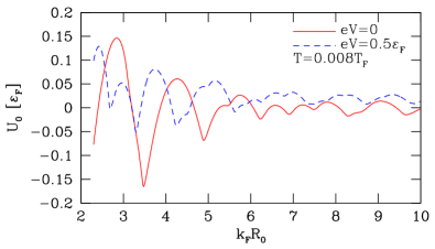
Figure 1: (Color online) The Hartree potential $U_{0}$ for electrons in a cylindrical nanowire at finite temperature $T=0.008\,T_{F}$, with a symmetric potential drop, versus the radius $R_{0}$ of the wire.

For an unperturbed cylinder, the mesoscopic Hartree potential $U_{0}$ that simultaneously solves Eqs. (14) and (17) is only a function of the radius $R_{0}$, voltage $eV=\mu_{+}-\mu_{-}$, and temperature $T$, and is constant along the wire, neglecting boundary effects, which are important only within a screening length ($\mbox{}\sim k_{F}^{-1}$) of each contact. (This description is valid for wires with $1\ll k_{F}L<k_{F}L_{\rm in}$.) $U_{0}$ is independent of the choice of $\eta$ in the Coulomb interaction, Eq. (9), and can be determined by the charge neutrality condition

$$Q=\frac{1}{2}e[N_{-}(\mu_{+}-U_{0})+N_{-}(\mu_{-}-U_{0})]-eN_{+}=0,$$ (20)

where $\frac{1}{2}N_{-}(\mu=\mu_{\pm}-U_{0})=\frac{1}{2}\int_{0}^{L}\!dz\int^{\mu}\!dE\,g_{T}(z,E)$ is the number of right(left)-moving electrons in the cylindrical wire, and $N_{+}$ is the total number of background positive charges. Equation (20) gives a relationChristen and Büttiker (1996)

$$U_{0}=U_{0}^{(s)}(R_{0},V,T)+\frac{1}{2}(\mu_{+}+\mu_{-})-\varepsilon_{F},$$ (21)

where $U_{0}^{(s)}$ is calculated with a symmetric voltage drop $V_{+}=-V_{-}=\frac{1}{2}V$. Equation (21) guarantees that all physical properties of the system calculated in the following are just functions of the voltage $V$, and not of $\mu_{+}$ and $\mu_{-}$ separately.

Using these expressions, one can solve Eq. (20) for $U_{0}$ for a symmetric potential drop, $\mu_{\pm}=\varepsilon_{F}\pm\frac{1}{2}eV$. The solution is shown in Fig. 1 as a function of radius $R_{0}$ at two different voltages $V$. In the equilibrium case ($V=0$), $U_{0}$ oscillates about zero, exhibiting cusps at the subband thresholds, and increasing in amplitude as $R_{0}$ decreases, due to the quantum confinement. Note that in equilibrium, $U_{0}\rightarrow 0$ as $R_{0}\rightarrow\infty$, consistent with the well-known behavior of bulk jellium. At finite bias, each cusp in $U_{0}$ splits in two, corresponding to the subband thresholds for left- and right-moving electrons:

$$\mu_{\pm}=\varepsilon_{\nu}(R_{0})+U_{0}(R_{0},V,T),$$ (22)

where $\varepsilon_{\nu}(R_{0})$ are the eigenenergies of a disk billiard of radius $R_{0}$. This is illustrated in Fig. 1 for $eV=0.5\varepsilon_{F}$. Note that in addition to the splitting, there is a substantial shift of the peak structure at finite bias.

Using Eq. (10), the grand canonical potential of a cylinder is now found to be

$$\Omega(R_{0},V,T)=\Omega_{0}[\{\mu_{\pm}\},R_{0},U_{0}]-N_{+}U_{0}.$$ (23)

Note that $\Omega$ is invariant under a global shift of the potential $U_{0}$, due to an exact cancellation in the two terms on the r.h.s. of Eq. (23). The tensile force in the nanowire provides direct information about cohesion, and is given by

$$F(R_{0},V,T)=-\left.\frac{\partial\Omega}{\partial L}\right|_{R_{0}^{2}L,V,T}.$$

Figure 2 shows the tensile force of a metal nanocylinder as a function of its cross section for two different bias voltages. To facilitate comparison with the stability diagrams in Sec. IV below, the cross section is plotted in terms of the corrected Sharvin conductanceTorres et al. (1994)

$$G_{S}=G_{0}[(k_{F}R_{0}/2)^{2}-k_{F}R_{0}/2],$$ (24)

which gives a semiclassical approximation to the electrical conductance. In Fig. 2, $F<0$ corresponds to tension, while $F>0$ corresponds to compression. As shown below, the cusps in the cohesive force at the subband thresholds correspond to structural instabilities of the system.

Figure 2: (Color online) Tensile force in a metal nanocylinder versus cross-sectional area, at two different bias voltages at temperature $T=0.008\,T_{F}$. The cross section is plotted in terms of the Sharvin conductance $G_{S}$, Eq. (24), and the force is given in units of $\varepsilon_{F}/\lambda_{F}$ ($\lambda_{F}$ being the Fermi wavelength), which is $1.7$ nN for Au.

In Fig. 2, the force calculated at zero bias is very similar to previous resultsBlom et al. (1998); Höppler and Zwerger (1999); Stafford et al. (1999) based on the free-electron model, even though those calculations did not respect the charge neutrality (20) enforced by Coulomb interactions. The reason for the good agreement is that the contribution of the Hartree potential to the energy of the system is a second-order mesoscopic effect at zero bias,Stafford et al. (1999, 2000) which is essentially negligible for $G>3G_{0}$. An earlier calculationvan Ruitenbeek et al. (1997) that did invoke charge neutrality obtained a very different—and incorrect—result, because the second term on the r.h.s. of Eq. (23) was omitted, resulting in a double-counting of Coulomb interactions.

Figure 2 shows that the cohesive force of a metal nanowire can be modulated by several nano-Newtons for a bias of a few Volts. Such a large effect should be observable experimentally using appropriate cantilevers,Rubio et al. (1996); Stalder and Dürig (1996); Rubio-Bollinger et al. (2004) although the intrinsic behavior might be masked by electrostatic forces in the external circuit. In contrast to the case at $V=0$, the Coulomb interactions play an essential role in determining the cohesive force at finite bias, since the positions of the peaks depend sensitively on the Hartree potential $U_{0}$ of the ballistic nonequilibrium electron distribution, shown in Fig. 1. The gauge-invariant result shown in Fig. 2 thus differs substantially from previous results,Zagoskin (1998) where screening was not treated self-consistently. Gauge-invariant results for the nonlinear transport through metal nanocylinders will be presented elsewhere.Zhang

IV Linear Stability of a Cylinder at Finite Voltage

In this section, we perform a linear stability analysisKassubek et al. (2001); Zhang et al. (2003) for cylindrical nanowires under a finite bias $V$. Coulomb interactions are included self-consistently using the formalism of Sec. III. Although the details of the calculation are rather complicated, the method is conceptually straightforward: Having found the self-consistent solution (23) for a cylinder, we perturb the cylinder as in Eq. (15), and expand the free energy up to second order in the small parameter $\lambda$. First, the self-consistent integral equations (14) and (17) for the ballistic nonequilibrium electron distribution are solved using first-order perturbation theory in $\lambda$. Then the free energy is calculated using Eqs. (10) and (16).

The radius of the wire is given by Eq. (15), with a perturbation function

$$\delta R(z)=\sum_{q}b(q)e^{iqz},\quad\quad b(q)^{*}=b(-q).$$

The surface perturbation $\lambda\delta R(z)$ is subject to a constraint fixing the total number of atoms in the wire. In previous works, we have considered various constraints,Stafford et al. (1999); Urban et al. (2004b) which allow one to adjust the surface properties of the wire to model various materials. The simplest such constraint is volume conservation, under which the coefficient $b(0)$ is fixed by

$$b(0)=-\frac{\lambda}{2R_{0}}\sum_{q}|b(q)|^{2}.$$

Other reasonable constraints do not lead to qualitatively different conclusions.

Within linear response theory, we can expand $\delta\rho(z)$ around $U_{0}$ to linear order in $U(z)-U_{0}$, where $U_{0}$ is the mesoscopic Hartree potential for the corresponding unperturbed cylindrical wire. One gets

$$\delta\rho(z)\simeq\delta\rho_{0}(z)-\int\!dz^{\prime}\left.\frac{\delta\rho_{-}(z)}{\delta U(z^{\prime})}\right|_{U_{0}}U_{0}\\ +\int\!dz_{1}dz_{2}\left.\frac{\delta\rho_{-}(z)}{\delta U(z_{1})}\right|_{U_{0}}V(z_{1},z_{2})\delta\rho(z_{2}),$$ (25)

where Eq. (14) has been used and $\delta\rho_{0}(z)$, called the bare charge imbalance, is defined as

$$\delta\rho_{0}(z)=\frac{1}{2}\sum_{\alpha=\pm}\int^{\mu_{\alpha}-U_{0}}\!\!dE\,g_{T}(z,E)-\rho_{+}(z).$$ (26)

Now defining the dielectric function

$$\epsilon(z_{1},z_{2})=\delta(z_{1}-z_{2})-\int dz_{3}\left.\frac{\delta\rho_{-}(z_{1})}{\delta U(z_{3})}\right|_{U_{0}}V(z_{3},z_{2}),$$ (27)

we can rewrite Eq. (25) as

$$\delta\rho(z)=\int\!dz^{\prime}\epsilon^{-1}(z,z^{\prime})\delta\bar{\rho}_{0}(z^{\prime}),$$ (28)

where $\epsilon^{-1}$ is the inverse dielectric function which satisfies $\int dz_{3}\epsilon^{-1}(z_{1},z_{3})\epsilon(z_{3},z_{2})=\delta(z_{1}-z_{2})$, and

$$\delta\bar{\rho}_{0}(z)=\delta\rho_{0}(z)-\int\!dz_{1}\left.\frac{\delta\rho_{-}(z)}{\delta U(z_{1})}\right|_{U_{0}}U_{0}.$$ (29)

The functional derivative $\delta\rho_{-}(z)/\delta U(z^{\prime})$ can be calculated using Eq. (17), and is found to be

$$\left.\frac{\delta\rho_{-}(z)}{\delta U(z^{\prime})}\right|_{U_{0}}=-\frac{\delta(z-z^{\prime})}{2}\sum_{\alpha=\pm}g_{T}(z,\mu_{\alpha}-U_{0}).$$

Now we can expand the nonequilibrium grand canonical potential (10) as a series in $\lambda$. In order to do so, we first expand Eq. (10) around $U_{0}$. Using Eqs. (14), (17), (26) and (29), one gets

$$\Omega=\Omega_{0}[\{\mu_{\pm}\},R(z),U_{0}]-U_{0}\int_{0}^{L}\!dz\,\delta\bar{\rho}_{0}(z)\\ +\frac{1}{2}\int_{0}^{L}\!dz\,dz^{\prime}\,\delta\bar{\rho}_{0}(z)\tilde{V}(z,z^{\prime})\delta\bar{\rho}_{0}(z^{\prime})\\ +\frac{(U_{0})^{2}}{4}\sum_{\alpha=\pm}\int_{0}^{L}\!dz\,g_{T}(z,\varepsilon_{\alpha})-N_{+}U_{0},$$ (30)

where $\varepsilon_{\pm}=\mu_{\pm}-U_{0}$, and the screened potential $\tilde{V}(z,z^{\prime})$ is defined as

$$\tilde{V}(z,z^{\prime})=\int dz_{1}V(z,z_{1})\epsilon^{-1}(z_{1},z^{\prime}).$$ (31)

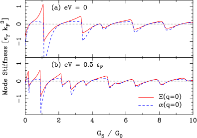
Figure 3: (Color online) Total mode stiffness $\Xi(q=0;R_{0},V,T)$, and leading-order contribution $\alpha(q=0;R_{0},V,T)$, at zero and finite bias, for $T=0.008\,T_{F}$.

At this point, all quantities have been expressed in terms of the local density of states $g_{T}(z,E)$ and the Coulomb interaction $V(z,z^{\prime})$, whose expansions in series of $\lambda$ are presented in Appendix A. In the end, the expansion of the grand canonical potential as a series in $\lambda$ is found to be

$$\Omega=\Omega(R_{0},V,T)+\lambda^{2}L\sum_{q>0}\Xi(q;R_{0},V,T)|b(q)|^{2}$$ (32)

plus terms ${\cal O}(\lambda^{3},L^{0})$, where $\Omega(R_{0},V,T)$ is given by Eq. (23), and the mode stiffness

$$\Xi(q;R_{0},V,T)\equiv\alpha(q;R_{0},V,T)\\ +\text{Re}\bigg{(}\frac{\hat{V}(q)}{\hat{\epsilon}(q)}\bigg{)}(\varrho^{(1)}_{1}-\varrho^{(1)}_{2}q^{2})^{2}.$$ (33)

Here $\hat{V}(q)$ and $\hat{\epsilon}(q)$ are, respectively, the Fourier transforms of $V^{(0)}(z)$ and $\epsilon^{(0)}(z)$, the Coulomb potential and dielectric function of an unperturbed cylinder. The factors $\varrho^{(1)}_{1}$ and $\varrho^{(1)}_{2}$ are given in Eqs. (42) and (43). The factor $\alpha(q;R_{0},V,T)$ comes from the expansion of $\Omega_{0}[\{\mu_{\pm}\},R(z),U_{0}]$ and is found to be

$$\alpha(q;R_{0},V,T)=-\frac{\pi\sigma_{s}}{R_{0}}\frac{\varepsilon_{+}^{2}+\varepsilon_{-}^{2}}{\varepsilon_{F}^{2}}\\ +\left(\pi\sigma_{s}R_{0}\frac{\varepsilon_{+}^{2}+\varepsilon_{-}^{2}}{\varepsilon_{F}^{2}}-\gamma_{s}\frac{\varepsilon_{+}^{3/2}+\varepsilon_{-}^{3/2}}{\varepsilon_{F}^{3/2}}\right)q^{2}\\ +\left(\frac{\partial^{2}}{\partial R_{0}^{2}}-\frac{1}{R_{0}}\frac{\partial}{\partial R_{0}}\right)V_{\rm shell}(R_{0},V,T),$$ (34)

where $\sigma_{s}$ is the surface tension, $\gamma_{s}$ is the curvature energy, and $V_{\rm shell}(R_{0},V,T)$ is the mesoscopic electron-shell potential,Bürki et al. (2003) given self-consistently at finite bias by

$$V_{\rm shell}(R_{0},V,T)=\frac{1}{\pi\varepsilon_{F}}\sum_{\alpha=\pm}\sum_{wv}\frac{a_{vw}(T)f_{vw}}{v^{2}L_{vw}}\\ \times\varepsilon_{\alpha}^{2}\cos(k_{F}^{\alpha}L_{vw}-3v\pi/2),$$ (35)

where $k_{F}^{\pm}=k_{F}\sqrt{\varepsilon_{\pm}/\varepsilon_{F}}$. In the present article, the valuesStafford et al. (1997) $\sigma_{s}=\varepsilon_{F}k_{F}^{2}/16\pi$ and $\gamma_{s}=2\varepsilon_{F}k_{F}/9\pi^{2}$, appropriate for a constant-volume constraint, are used throughout. Inserting material-specific valuesZhang et al. (2003) does not lead to a significant change in the stability diagram. Equations (32)–(35) represent the central result of this paper.

Figure 3 shows the long-wavelength mode stiffness $\Xi(q=0)$ at zero and finite bias. For comparison, the leading-order contribution $\alpha(q=0)$ is plotted as a dashed curve. The second term on the r.h.s. of Eq. (33), which is second-order in the induced charge imbalance, gives a significant contribution for small radii, but is negligible for $k_{F}R_{0}\gg 1$. Moreover, the sign of $\Xi$, which determines stability, is essentially fixed by $\alpha$ alone. The relative unimportance of the second-order correction is reminiscent of the Strutinsky theoremStrutinsky (1968); Ullmo et al. (2001) for finite fermion systems, which states that shell effects are dominated by the single-particle contribution in the mean-field potential.

Stability Diagram

The stability of a cylindrical nanowire of radius $R_{0}$ at bias $V$ and temperature $T$ is determined by the function $\Xi(q;R_{0},V,T)$: If $\Xi(q)>0$ $\forall q$, then the nanowire is stable with respect to small perturbations, and is a (meta)stable thermodynamic state. If $\Xi(q)<0$ for any $q$, then the wire is unstable.

Figure 4: (Color online) The factor $D(R_{0},V)$, coefficient of the $q^{2}$ contribution to $\Xi(q;R_{0},V)$, at temperature $T=0.008\,T_{F}$.

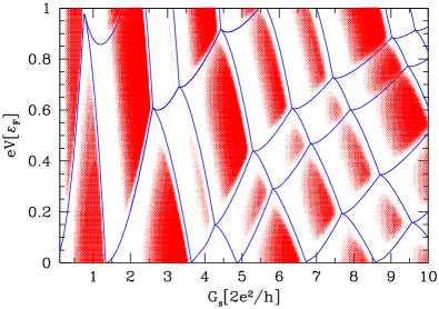
Figure 5: (Color online) Stability of cylindrical metal nanowires versus Sharvin conductance (24) and bias voltage. Shaded (red) areas indicate stability with respect to small perturbations at $T=0.008\,T_{F}$. Solid lines indicate subband thresholds for right- and left-moving electrons.

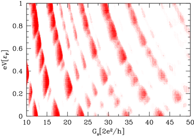
Figure 6: (Color online) Stability of cylindrical metal nanowires versus Sharvin conductance $G_{S}$ between $10$ and $50G_{0}$ and bias voltage. Shaded (red) areas indicate stability with respect to small perturbations at $T=0.008\,T_{F}$.

The second term on the r.h.s. of Eq. (33) is positive semidefinite, and thus cannot lead to an instability. The first term $\alpha(q)$ describes instabilities in two different regimes, as in the equilibrium case:Kassubek et al. (2001); Zhang et al. (2003) (i) The electron-shell contribution has deep negative peaks at the thresholds to open new conducting subbands (c.f. Fig. 3). (ii) The surface contribution to $\alpha(q)$ becomes negative for $qR_{0}<1$, the classical Rayleigh instability. From Eqs. (33) and (34), it is apparent that the most unstable mode (if any) within the semiclassical approximation is $q=0$, except for unphysical radii $R_{0}\lesssim\gamma_{s}/\sigma_{s}$ (less than one atom thick). To illustrate this point, the second derivative $D(R_{0},V,T)\equiv\left.\partial^{2}\Xi/\partial q^{2}\right|_{q=0}$ is shown in Fig. 4. Note that $D>0$ for $k_{F}R_{0}>3$.

The stability properties of the system are thus completely determinednot (b) by the sign of the stability function $A(R_{0},V,T)\equiv\Xi(q=0;R_{0},V,T)$. Figure 5 shows a stability diagram in the voltage $V$ and radius $R_{0}$ plane. The $x$-axis is given in terms of the Sharvin conductance (24), to facilitate the identification of the quantized (linear-response) conductance values of the stable nanowires. The shaded regions show nanowires that are stable with respect to small perturbations, with darker regions representing larger values of $A(R_{0},V,T)$. In the figure, the solid lines show the subband thresholds for right- and left-moving electrons, which are determined by Eq. (22). At the temperature shown $T=0.008T_{F}$, which corresponds roughly to room temperature, the electron-shell effect dominates, leading to instabilities at the subband thresholds, and stabilizing the wire in some of the intervening fingers.

A stability diagram up to $G_{S}=50G_{0}$ is shown in Fig. 6, where the subband thresholds have been omitted to avoid clutter. Figures 5 and 6 show that cylindrical metal nanowires with certain magic conductance values $G/G_{0}=1,3,6,12,17,23,34,42,\ldots$ remain linearly stable at room temperature up to bias voltages $eV\sim 0.1\varepsilon_{F}$ or higher. These ballistic conductors can therefore support extremely high current densities, of order $10^{11}\mbox{A}/\mbox{cm}^{2}$ by Eq. (1). These are precisely the same magic cylinders which were previously found to be linearly stable at zero bias up to very high temperatures.Zhang et al. (2003) Cylinders with $G/G_{0}=8$ and 10 are also predicted to be stable at finite bias, but not as robust as the neighboring configurations with $G/G_{0}=6$ and 12.

It should be mentioned that in addition to the stable cylindrical configurations shown in Figs. 5 and 6, nanowires with elliptical cross sections and conductance $G/G_{0}=2,5,9,29,\ldots$ were also found to be stable at zero bias,Urban et al. (2004b) although their finite-bias stability has not yet been investigated.

Perhaps the most startling prediction of Figs. 5 and 6 is that there are a number of cylindrical nanowire structures which are stable with respect to small perturbations at finite bias, but unstable in equilibrium! These metastable structures could lead to additional peaks in conductance histograms at finite bias, which are not present at low bias. It may also be possible to observe switching behavior between the various stable structures as the voltage is varied.

The results of the above stability analysis should be directly relevant for nanowires made of simple monovalent metals, such as alkali metals and, to some extent, noble metals. Indeed, the calculated bias dependence of the stability of metal nanocylinders with conductance $G/G_{0}=1$ and 3, shown in Fig. 5, is consistent with experimental histograms for gold nanocontacts,Yasuda and Sakai (1997) where a peak at $G\approx G_{0}$ was found up to 1.9V at room temperature, and a peak at $G\approx 3G_{0}$ was found up to about 1.5V. Similar experimental results have been obtained by several groups.Itakura et al. (1999); Untiedt et al. (2000); Hansen et al. (2000); Yuki et al. (2001); Mehrez et al. (2002); Agraït et al. (2002) Our analysis strongly suggests that the remarkable stability properties of gold nanowires at finite bias are not a special property of gold, but rather a generic feature of metal nanoconductors.

Nature of the instability

The nature of the predicted instability of metal nanocylinders at finite bias may be illuminated by means of a nontrivial identityZhang et al. (2003) linking Eqs. (23) and (33):

$$\lim_{q\rightarrow 0}\Xi(q;R_{0},V,T)=\left(\frac{\partial^{2}}{\partial R_{0}^{2}}-\frac{1}{R_{0}}\frac{\partial}{\partial R_{0}}\right)\frac{\Omega(R_{0},V,T)}{L}.$$ (36)

This implies that the instability corresponds to a homogeneous-inhomogeneous transition,Zhang et al. (2003) since the r.h.s. of Eq. (36) is proportional to the energetic cost of a volume-conserving phase separation into thick and thin segments. In the inhomogeneous phase at finite bias, the surface corrugation will not be static, but will diffuse like a defect undergoing electromigration.Yasuda and Sakai (1997); Ralls et al. (1989); Holweg et al. (1992) The stable nanocylinders are immune to electromigration, because they are translationally invariant and they are so thin that they are defect free. Electromigration is possible only if a surface-defect is nucleated,Bürki et al. (2004) which becomes energetically favorable on the stability boundary. The predicted surface instability may thus represent the ultimate nanoscale limit of electromigration.

V Conclusions

In this paper, we develop a self-consistent scattering approach to the nonequilibrium thermodynamics of open mesoscopic systems, and use it to study the cohesion and stability of metal nanocylinders under finite bias. In our approach, the positive ions are modeled as an incompressible fluid, and interactions are treated in the Hartree approximation, using a quasi-one-dimensional form of the Coulomb interaction. This single-band model is appropriate for simple monovalent metals. It is especially suited to alkali metals, but is also appropriate to describe quantum shell effects due to the conduction-band $s$ electrons in noble metals.

We have utilized a semiclassical treatment of the electron-shell structure that plays a crucial role in stabilizing metal nanowires at finite bias. Previous studies Urban and Grabert (2003); Urban et al. (2004b) have shown that this semiclassical approach accurately describes the energetic cost of long-wavelength surface perturbations, which are the limiting factor Zhang et al. (2003) in the structural stability of long nanowires. Furthermore, we have assumed a ballistic nonequilibrium electron distribution in the nanowire at finite bias, neglecting inelastic electron-phonon and electron-electron scattering. This approximation is valid for wires shorter than the inelastic mean-free path.

We find that the tensile force in a nanowire can be modulated by several nano-Newtons when biased by a few volts. Such a large effect should be observable experimentally,Rubio et al. (1996); Stalder and Dürig (1996); Rubio-Bollinger et al. (2004) although the intrinsic behavior might be masked by electrostatic forces in the external circuit.

The principal result of this paper is a linear stability analysis of metal nanowires at finite bias, which reveals that cylindrical wires with certain magic conductance values $G/G_{0}=1,3,6,12,17,23,34,42,\ldots$ remain stable up to bias voltages $eV\sim 0.1\,\varepsilon_{F}$ or higher, with the maximum sustainable bias decreasing with increasing radius. In particular, wires with $G/G_{0}=1$ and $3$ are predicted to be stable up to $eV\sim 0.5\,\varepsilon_{F}$. This maximum voltage is slightly larger than what is observed experimentally.Yasuda and Sakai (1997); Agraït et al. (2002) It should, however, be pointed out that stability with respect to small perturbations is not a sufficient condition for a nanowire to be observed: Metal nanowires are metastable structures, and can be observed only if their lifetime is sufficiently long on the experimental timescale. As a result, the observed maximum sustainable bias is likely to be somewhat smaller than that predicted by a linear stability analysis.

A striking prediction of our stability analysis is the existence of nanowire structures (e.g. cylinders with conductance $G/G_{0}=2,5,7,9,14,20,\ldots$) that are only stable under an applied bias. This suggests that conductance histograms taken at finite voltage might have additional peaks, or even a completely different set of peaks, compared to zero-voltage histograms. It may also be possible to observe switching between different stable structures as a function of voltage.

Metal nanowires with elliptical cross sections and conductance $G/G_{0}=2,5,9,29,\ldots$ are also predicted to be stable at zero bias.Urban et al. (2004b) Although some of the conductance values of the elliptical wires coincide with those of cylindrical wires predicted to be stable only at finite bias, it should be possible to distinguish these geometries experimentally due to the different kinetic pathways involved in their formation, and the very different bias dependence of their stability.

Finally, we point out that the predicted instability of metal nanowires at finite bias may represent the ultimate nanoscale limit of electromigration, due to the current-induced nucleation of surface modulation in an otherwise perfect, translationally invariant nanowire.

Appendix A Expansion of the Non-Equilibrium Free Energy

In this appendix, we present more details of the derivation of Eqs. (30) and (32).

Local Density of States $g_{T}(z,E)$

In order to include the temperature in the semiclassical formalism, we use a convoluted density of states $g_{T}(z,E)=\int\left(-\partial f_{0}(E-E^{\prime})/\partial E\right)g(z,E^{\prime})dE^{\prime}$, where $f_{0}(E)=[1+\exp(\beta E)]^{-1}$. Thermodynamic quantities are then obtained through their zero-temperature expression with the density of states $g(E)$ replaced by $g_{T}(E)$. The temperature dependence of the average part $\bar{g}_{T}(z,E)$, proportional to $(1+{\cal O}(T/T_{F})^{2})\approx 1$, ($T_{F}$ is the Fermi temperature), is negligible, while the temperature dependence of the fluctuating part $\delta g_{T}(z,E)$ is included in the damping factor $a_{vw}(T)$ [see Eq. (19)]. In the following, we set the factor $a_{vw}(T)$ equal to its unperturbed value at the Fermi energy $\varepsilon_{F}$, since the variation of this factor with the perturbation or with energy does not give an important contribution. We also drop the subscript $T$ for the convoluted density of states to simplify the notation.

For a perturbed cylinder, the average part of the density of states, Eq. (18), can be expanded to second order in the small parameter $\lambda$ as

$$\bar{g}(z,E)\simeq\bar{g}^{(0)}+\lambda\bar{g}^{(1)}+\lambda^{2}\bar{g}^{(2)},$$ (37)

where

$$\bar{g}^{(0)} = \frac{k_{F}^{3}R_{0}^{2}}{2\pi\varepsilon_{F}}\sqrt{\frac{E}{\varepsilon_{F}}}-\frac{k_{F}^{2}R_{0}}{4\varepsilon_{F}}+\frac{k_{F}}{6\pi\varepsilon_{F}}\sqrt{\frac{\varepsilon_{F}}{E}},$$

$$\bar{g}^{(1)} = \left(\frac{k_{F}^{3}R_{0}}{\pi\varepsilon_{F}}\sqrt{\frac{E}{\varepsilon_{F}}}-\frac{k_{F}^{2}}{4\varepsilon_{F}}\right)\delta R(z)$$

$$-\frac{k_{F}R_{0}}{6\pi\varepsilon_{F}}\sqrt{\frac{\varepsilon_{F}}{E}}\delta R^{\prime\prime}(z),$$

$$\bar{g}^{(2)} = \frac{k_{F}^{3}}{2\pi\varepsilon_{F}}\sqrt{\frac{E}{\varepsilon_{F}}}\delta R^{2}(z)-\frac{k_{F}^{2}R_{0}}{8\varepsilon_{F}}\delta R^{\prime\,2}(z)$$

$$-\frac{k_{F}}{6\pi\varepsilon_{F}}\sqrt{\frac{\varepsilon_{F}}{E}}\delta R(z)\delta R^{\prime\prime}(z),$$

and the prime denotes differentiation with respect to $z$.

Similarly, the fluctuating part of the density of states for a small deformation of a cylinder, Eq. (19), can be calculated using semiclassical perturbation theory,Kassubek et al. (2001); Stafford et al. (2001) and is found to be

$$\delta g(z,E)\simeq\delta g^{(0)}(E)+\lambda\delta g^{(1)}(z,E)+\lambda^{2}\delta g^{(2)}(z,E),$$ (38)

with

$$\delta g^{(0)}=\frac{k_{F}^{2}}{2\pi\varepsilon_{F}}\sum_{wv}\frac{a_{vw}(T)f_{vw}L_{vw}}{v^{2}}\cos\theta_{vw}(E),$$

$$\delta g^{(1)}=\frac{k_{F}^{2}}{2\pi\varepsilon_{F}}\sum_{wv}\frac{a_{vw}(T)f_{vw}L_{vw}}{v^{2}R_{0}}\delta R(z)\\ \times\left[\cos\theta_{vw}(E)-k_{E}L_{vw}\sin\theta_{vw}(E)\right],$$

$$\delta g^{(2)}=-\frac{k_{F}^{2}}{2\pi\varepsilon_{F}}\sum_{wv}\frac{a_{vw}(T)f_{vw}L_{vw}^{2}}{2v^{2}R_{0}^{2}}k_{E}\delta R^{2}(z)\\ \times\left[2\sin\theta_{vw}(E)+k_{E}L_{vw}\cos\theta_{vw}(E)\right].$$

where, once more, the sum is over all classical periodic orbits $(v,w)$ in a disk billiard of radius $R_{0}$, the factor $f_{vw}=1$ for $v=2w$ and 2 otherwise accounts for the invariance under time-reversal symmetry of some orbits, $L_{vw}=2vR_{0}\sin(\pi w/v)$ is the length of periodic orbit $(v,w)$, $\theta_{vw}(E)=k_{F}L_{vw}\sqrt{E/\varepsilon_{F}}-3v\pi/2$, and $a_{vw}(T)=\tau_{vw}/\sinh\tau_{vw}$, with $\tau_{vw}=\pi k_{F}L_{vw}T/2T_{F}$, is a temperature dependent damping factor.

To shorten subsequent equations, we define the functions of energy $g^{(i)}_{j}(E)$ by writing the first- and second-order contributions to the local density of states as

$$g^{(1)}(z,E) =g^{(1)}_{1}(E)\delta R(z)+g^{(1)}_{2}(E)\delta R^{\prime\prime}(z),$$ (39)

$$g^{(2)}(z,E) =g^{(2)}_{1}(E)\delta R^{2}(z)+g^{(2)}_{2}(E)\delta R^{\prime 2}(z)$$

$$\quad+g^{(2)}_{3}(E)\delta R(z)\delta R^{\prime\prime}(z).$$ (40)

The total density of states per unit length of a cylindrical wire is $g^{(0)}(E)=\bar{g}^{(0)}(E)+\delta g^{(0)}(E)$.

Bare charge imbalances $\delta\rho_{0}(z)$ and $\delta\bar{\rho}_{0}(z)$

Now substituting the expansion of the local density of states into Eq. (26), one gets the expansion of $\delta\rho_{0}(z)$ as

$$\delta\rho_{0}(z)\simeq\lambda\delta\rho_{0}^{(1)}+\lambda^{2}\delta\rho_{0}^{(2)},$$ (41)

with

$$\delta\rho^{(1)}_{0}(z)=\varrho^{(1)}_{1}\delta R(z)+\varrho^{(1)}_{2}\delta R^{\prime\prime}(z),$$

where the coefficients $\varrho^{(1)}_{1}$ and $\varrho^{(1)}_{2}$ are defined as

$$\varrho^{(1)}_{1}=\frac{k_{F}^{3}R_{0}}{3\pi}\left(\frac{\varepsilon_{+}^{3/2}+\varepsilon_{-}^{3/2}}{\varepsilon_{F}^{3/2}}-2\right)\\ -\frac{k_{F}^{2}}{8}\left(\frac{\varepsilon_{+}+\varepsilon_{-}}{\varepsilon_{F}}-2\right)+\frac{\delta\varrho^{(1)}_{+}+\delta\varrho^{(1)}_{-}}{2},$$ (42)

$$\varrho^{(1)}_{2}=-\frac{k_{F}R_{0}}{6\pi}\left(\frac{\varepsilon_{+}^{1/2}+\varepsilon_{-}^{1/2}}{\varepsilon_{F}^{1/2}}-2\right),\hfill$$ (43)

with $\varepsilon_{\pm}=\mu_{\pm}-U_{0}$, and

$$\delta\varrho^{(1)}_{\pm}=\frac{k_{F}^{2}\varepsilon_{\pm}}{\pi\varepsilon_{F}}\sum_{vw}\frac{f_{vw}a_{vw}(T)}{v^{2}R_{0}}\\ \times\bigg{(}L_{vw}\cos\theta_{vw}(\varepsilon_{\pm})+k_{\pm}^{-1}\sin\theta_{vw}(\varepsilon_{\pm})\bigg{)},$$

where $k_{\pm}=k_{F}\sqrt{\varepsilon_{\pm}/\varepsilon_{F}}$, while

$$\delta\rho^{(2)}_{0}(z)=\varrho^{(2)}_{1}\delta R^{2}(z)+\varrho^{(2)}_{2}\delta R^{\prime\,2}(z)+\varrho^{(2)}_{3}\delta R(z)\delta R^{\prime\prime}(z),$$

where coefficients $\varrho^{(2)}_{1},\varrho^{(2)}_{2}$ and $\varrho^{(2)}_{3}$ are

$$\varrho^{(2)}_{1} =\frac{k_{F}^{3}}{6\pi}\left(\frac{\varepsilon_{+}^{3/2}+\varepsilon_{-}^{3/2}}{\varepsilon_{F}^{3/2}}-2\right)+\frac{\delta\varrho^{(2)}_{+}+\delta\varrho^{(2)}_{-}}{2},$$

$$\varrho^{(2)}_{2} =-\frac{k_{F}^{2}R_{0}}{16}\left(\frac{\varepsilon_{+}+\varepsilon_{-}}{\varepsilon_{F}}-2\right),\quad\varrho^{(2)}_{3}=\frac{\varrho^{(1)}_{2}}{R_{0}},$$

and

$$\delta\varrho^{(2)}_{\pm}=-\frac{k_{F}^{2}}{2\pi}\frac{\varepsilon_{\pm}}{\varepsilon_{F}}\sum_{vw}\frac{f_{vw}a_{vw}(T)}{v^{2}R_{0}^{2}}L_{vw}\\ \times\bigg{(}L_{vw}\sin\theta_{vw}(\varepsilon_{\pm})-2k_{\pm}^{-1}\cos\theta_{vw}(\varepsilon_{\pm})\bigg{)}.$$

Similarly, Eq. (29) for $\delta\bar{\rho}_{0}(z)$ is expanded as

$$\delta\bar{\rho}_{0}(z,E)\simeq\delta\bar{\rho}_{0}^{(0)}+\lambda\delta\bar{\rho}_{0}^{(1)}+\lambda^{2}\delta\bar{\rho}_{0}^{(2)},$$ (44)

with

$$\delta\bar{\rho}^{(0)}_{0} = \frac{U_{0}}{2}\left[g^{(0)}(\varepsilon_{+})+g^{(0)}(\varepsilon_{-})\right],$$

$$\delta\bar{\rho}^{(1)}_{0} = \bar{\varrho}^{(1)}_{1}\delta R(z)+\bar{\varrho}^{(1)}_{2}\delta R^{\prime\prime}(z),$$

$$\delta\bar{\rho}^{(2)}_{0} = \bar{\varrho}^{(2)}_{1}\delta R^{2}(z)+\bar{\varrho}^{(2)}_{2}\delta R^{\prime 2}(z)+\bar{\varrho}^{(2)}_{3}\delta R(z)\delta R^{\prime\prime}(z),$$

where $\bar{\varrho}^{(i)}_{j}\equiv\varrho^{(i)}_{j}+\frac{1}{2}U_{0}[g^{(i)}_{j}(\varepsilon_{+})+g^{(i)}_{j}(\varepsilon_{-})]$.

Effective Coulomb potential $V(z,z^{\prime})$

The expansion of the Coulomb potential (9) as a series in $\lambda$ gives

$$V(z,z^{\prime})\simeq V^{(0)}(z-z^{\prime})\\ +\lambda\,V^{(1)}(z,z^{\prime})+\lambda^{2}\,V^{(2)}(z,z^{\prime}),$$ (45)

where

$$V^{(0)}(z) =\frac{e^{2}}{\sqrt{z^{2}+\eta R_{0}^{2}}},$$

$$V^{(1)}(z,z^{\prime}) =\frac{\delta R(z)+\delta R(z^{\prime})}{2}\cdot\frac{dV^{(0)}(z-z^{\prime})}{dR_{0}},$$

$$V^{(2)}(z,z^{\prime}) =\frac{1}{8}\left([\delta R(z)+\delta R(z^{\prime})]^{2}\frac{d}{dR_{0}}\right.$$

$$\qquad\left.+\frac{[\delta R(z)-\delta R(z^{\prime})]^{2}}{R_{0}}\right)\frac{dV^{(0)}(z-z^{\prime})}{dR_{0}}.$$

For future use, let us define the Fourier transform of $V^{(0)}(z)$ as

$$\hat{V}(q)=\int_{0}^{L}\!dz\,e^{-iqz}V^{(0)}(z).$$ (46)

Note that $\text{Re}\hat{V}(q)>0$.

Inverse dielectric function $\epsilon^{-1}(z,z^{\prime})$

We first expand the dielectric function $\epsilon(z,z^{\prime})$, Eq. (27), as

$$\epsilon(z,z^{\prime})=\epsilon^{(0)}(z-z^{\prime})\\ +\lambda\,\epsilon^{(1)}(z,z^{\prime})+\lambda^{2}\,\epsilon^{(2)}(z,z^{\prime}),$$ (47)

where the zeroth-order term is

$$\epsilon^{(0)}(z)=\delta(z)+\frac{g^{(0)}(\varepsilon_{+})+g^{(0)}(\varepsilon_{-})}{2}V^{(0)}(z),$$ (48)

the first-order term is

$$\epsilon^{(1)}(z,z^{\prime})=\frac{1}{2}\sum_{\alpha=\pm}\big{(}g^{(1)}(z,\varepsilon_{\alpha})V^{(0)}(z-z^{\prime})\\ +g^{(0)}(z,\varepsilon_{\alpha})V^{(1)}(z,z^{\prime})\big{)},$$

and the second-order term is

$$\epsilon^{(2)}(z,z^{\prime})=\frac{1}{2}\sum_{\alpha=\pm}\Big{(}g^{(2)}(z,\varepsilon_{\alpha})V^{(0)}(z-z^{\prime})\\ +g^{(1)}(z,\varepsilon_{\alpha})V^{(1)}(z,z^{\prime})+g^{(0)}(z,\varepsilon_{\alpha})V^{(2)}(z,z^{\prime})\Big{)}.$$

Let us define the Fourier transform of $\epsilon^{(0)}(z)$ as

$$\begin{split}\hat{\epsilon}(q)&=\int_{0}^{L}\!dz\,e^{-iqz}\epsilon^{(0)}(z)\\ &=1+\frac{g^{(0)}(\varepsilon_{+})+g^{(0)}(\varepsilon_{-})}{2}\hat{V}(q).\end{split}$$ (49)

Note that $\text{Re}\left(\hat{\epsilon}(q)/\hat{V}(q)\right)>0$, since both $g^{(0)}(\varepsilon)>0$ and $\hat{V}(q)>0$. Substituting Eq. (47) into the identity

$$\int\!dz^{\prime\prime}\,\epsilon^{-1}(z,z^{\prime\prime})\epsilon(z^{\prime\prime},z^{\prime})=\delta(z-z^{\prime}),$$

one can solve order by order for the inverse dielectric function $\epsilon^{-1}(z,z^{\prime})$

$$\epsilon^{-1}(z,z^{\prime})=\epsilon^{-1,(0)}(z-z^{\prime})\\ +\lambda\,\epsilon^{-1,(1)}(z,z^{\prime})+\lambda^{2}\,\epsilon^{-1,(2)}(z,z^{\prime}),$$ (50)

where the zeroth-order term is

$$\epsilon^{-1,(0)}(z)=\frac{1}{L}\sum_{q}\frac{e^{iqz}}{\hat{\epsilon}(q)},$$

the first-order term is found to be

$$\epsilon^{-1,(1)}=-\int\!dz_{1}\!\int\!dz_{2}\,\epsilon^{-1,(0)}(z-z_{1})\\ \times\epsilon^{(1)}(z_{1},z_{2})\,\epsilon^{-1,(0)}(z_{2}-z^{\prime}),$$

and the second-order term is

$$\epsilon^{-1,(2)}(z,z^{\prime})=-\int\!dz_{1}\!\int\!dz_{2}\,\epsilon^{-1,(0)}(z_{2}-z^{\prime})\\ \times\bigg{[}\epsilon^{-1,(0)}(z-z_{1})\,\epsilon^{(2)}(z_{1},z_{2})\\ +\epsilon^{-1,(1)}(z-z_{1})\,\epsilon^{(1)}(z_{1},z_{2})\bigg{]}.$$

Screened Potential $\tilde{V}(z,z^{\prime})$

Substituting the expansions (45) and (50) of $V$ and $\epsilon^{-1}$ into Eq. (31), one gets an expansion of the screened potential as

$$\tilde{V}(z,z^{\prime})=\tilde{V}^{(0)}(z-z^{\prime})\\ +\lambda\,\tilde{V}^{(1)}(z,z^{\prime})+\lambda^{2}\,\tilde{V}^{(2)}(z,z^{\prime})$$ (51)

where the zeroth-order term is

$$\tilde{V}^{(0)}(z)=\int\!dz_{1}\,V^{(0)}(z-z_{1})\epsilon^{-1,(0)}(z_{1})=\frac{1}{L}\sum_{q}\frac{\hat{V}(q)}{\hat{\epsilon}(q)}e^{\displaystyle iqz},$$

the first-order term is

$$\tilde{V}^{(1)}(z,z^{\prime})=\int\!dz_{1}\bigg{[} V^{(0)}(z-z_{1})\epsilon^{-1,(1)}(z_{1},z^{\prime})$$

$$+V^{(1)}(z-z_{1})\epsilon^{-1,(0)}(z_{1}-z^{\prime})\bigg{]},$$

while the second-order term is

$$\tilde{V}^{(2)}(z,z^{\prime})=\int\!dz_{1}\bigg{[} V^{(0)}(z-z_{1})\epsilon^{-1,(2)}(z_{1},z^{\prime})$$

$$+V^{(1)}(z-z_{1})\epsilon^{-1,(1)}(z_{1},z^{\prime})$$

$$+V^{(2)}(z-z_{1})\epsilon^{-1,(0)}(z_{1}-z^{\prime})\bigg{]}.$$

Grand canonical potential $\Omega[V,R(z),U(z)]$

Using Eqs. (37), (38), (41), (44), and (51) for $g(z,E)$, $\delta\rho_{0}$, $\delta\bar{\rho}_{0}$, and $\tilde{V}$, we are now ready to expand $\Omega$, starting by rewriting Eq. (30) as

$$\Omega\simeq\Omega_{0}[\{\mu_{\pm}\},R(z),U_{0}]-N_{+}U_{0}\\ -\Omega_{1}[\{\mu_{\pm}\},R(z),U_{0}]+\Omega_{2}[\{\mu_{\pm}\},R(z),U_{0}]\\ +\Omega_{3}[\{\mu_{\pm}\},R(z),U_{0}],$$ (52)

where

$$\Omega_{1}=U_{0}\int\!dz\,\delta\bar{\rho}_{0}(z)\\ \quad\,\,=U_{0}L\Bigg{[}\frac{U_{0}}{2}\sum_{\alpha=\pm}g^{(0)}(\varepsilon_{\alpha})+\lambda\bar{\varrho}^{(1)}_{1}b(0)\\ +\lambda^{2}\sum_{q}\left[\bar{\varrho}^{(2)}_{1}+(\bar{\varrho}^{(2)}_{2}-\bar{\varrho}^{(2)}_{3})q^{2}\right]|b(q)|^{2}\Bigg{]},$$

$$\Omega_{2}=\frac{(U_{0})^{2}}{4}\sum_{\alpha=\pm}\int\!dz\,g(z,\varepsilon_{\alpha})\\ \quad\,\,=\frac{(U_{0})^{2}}{4}L\sum_{\alpha=\pm}\Bigg{[}g^{(0)}(\varepsilon_{\alpha})+\lambda g^{(1)}_{1}(\varepsilon_{\alpha})b(0)\\ +\lambda^{2}\sum_{q}\left[g^{(2)}_{1}(\varepsilon_{\alpha})+[g^{(2)}_{2}(\varepsilon_{\alpha})-g^{(2)}_{3}(\varepsilon_{\alpha})]q^{2}\right]|b(q)|^{2}\Bigg{]},$$

and $\Omega_{3}=\frac{1}{2}\int dzdz^{\prime}\delta\bar{\rho}_{0}(z)\tilde{V}(z,z^{\prime})\delta\bar{\rho}_{0}(z)$ can be written as

$$\Omega_{3}[\{\mu_{\pm}\},R(z),U_{0}]=\Omega_{3}^{(0)}[\{\mu_{\pm}\},R_{0},U_{0}]\\ +\lambda\,\Omega_{3}^{(1)}[\{\mu_{\pm}\},R_{0},U_{0}]+\lambda^{2}\,\Omega_{3}^{(2)}[\{\mu_{\pm}\},R_{0},U_{0}].$$

The zeroth order term in the expansion of $\Omega_{3}$ is

$$\Omega^{(0)}_{3} =\frac{1}{2}\int\!dzdz^{\prime}\,\delta\bar{\rho}^{(0)}_{0}(z)\tilde{V}^{(0)}(z-z^{\prime})\delta\bar{\rho}^{(0)}_{0}(z^{\prime})$$

$$=\frac{L}{4}(U_{0})^{2}\sum_{\alpha=\pm}g^{(0)}(\varepsilon_{\alpha}),$$

the first-order term is

$$\Omega^{(1)}_{3} =\frac{1}{2}\int\!dzdz^{\prime}\,\bigg{[}\delta\bar{\rho}^{(0)}_{0}(z)\tilde{V}^{(1)}(z,z^{\prime})\delta\bar{\rho}^{(0)}_{0}(z^{\prime})$$

$$\hskip 62.59596pt+2\delta\bar{\rho}^{(1)}_{0}(z)\tilde{V}^{(0)}(z-z^{\prime})\delta\bar{\rho}^{(0)}_{0}(z^{\prime})\bigg{]}$$

$$=LU_{0}\bar{\varrho}_{1}^{(1)}b(0)+{\cal O}(L^{0}),$$

and the second-order contribution is

$$\Omega^{(2)}_{3} =\frac{1}{2}\int\!dzdz^{\prime}\,\Big{[}\delta\bar{\rho}^{(0)}_{0}(z)\tilde{V}^{(2)}(z,z^{\prime})\delta\bar{\rho}^{(0)}_{0}(z^{\prime})$$

$$\hskip 62.59596pt+2\delta\bar{\rho}^{(0)}_{0}(z)\tilde{V}^{(1)}(z,z^{\prime})\delta\bar{\rho}^{(1)}_{0}(z^{\prime})$$

$$\hskip 62.59596pt+2\delta\bar{\rho}^{(2)}_{0}(z)\tilde{V}^{(0)}(z-z^{\prime})\delta\bar{\rho}^{(0)}_{0}(z^{\prime})$$

$$\hskip 62.59596pt+\delta\bar{\rho}^{(1)}_{0}(z)\tilde{V}^{(0)}(z-z^{\prime})\delta\bar{\rho}^{(1)}_{0}(z^{\prime})\Big{]}$$

$$=LU_{0}\sum_{q}\Big{[}\varrho_{1}^{(2)}+(\varrho_{2}^{(2)}-\varrho_{3}^{(2)})q^{2}\Big{]}|b(q)|^{2}$$

$$\quad+\frac{L}{2}\sum_{q}\frac{\hat{V}(q)}{\hat{\epsilon}(q)}\Big{[}\varrho_{1}^{(1)}-\varrho_{2}^{(1)}q^{2}\Big{]}^{2}|b(q)|^{2}+{\cal O}(L^{0}).$$

Adding up all the contributions in Eq. (52), and dropping contributions of order $L^{0}$, one gets Eqs. (32) and (33).

The above calculations also show that Eq. (30) can be rewritten as

$$\Omega=\Omega_{0}[\{\mu_{\pm}\},R(z),U_{0}]-N_{+}U_{0}\\ +\frac{1}{2}\int\!dzdz^{\prime}\,\delta\rho_{0}^{(1)}(z)\tilde{V}^{(0)}(z-z^{\prime})\delta\rho_{0}^{(1)}(z^{\prime})\\ +{\cal O}(L^{0}).$$ (53)

References

- Agraït et al. (2003) N. Agraït, A. Levy Yeyati, and J. M. van Ruitenbeek, Phys. Rep. 377, 81 (2003).
- Yasuda and Sakai (1997) H. Yasuda and A. Sakai, Phys. Rev. B 56, 1069 (1997).
- Itakura et al. (1999) K. Itakura, K. Yuki, S. Kurokawa, H. Yasuda, and A. Sakai, Phys. Rev. B 60, 11163 (1999).
- Untiedt et al. (2000) C. Untiedt, G. Rubio Bollinger, S. Vieira, and N. Agraït, Phys. Rev. B 62, 9962 (2000).
- Hansen et al. (2000) K. Hansen, S. K. Nielsen, M. Brandbyge, E. Lægsgaard, I. Stensgaard, and F. Besenbacher, Appl. Phys. Lett. 77, 708 (2000).
- Yuki et al. (2001) K. Yuki, A. Enomoto, and A. Sakai, Appl. Surf. Sci. 169–170, 489 (2001).
- Mehrez et al. (2002) H. Mehrez, A. Wlasenko, B. Larade, J. Taylor, P. Grutter, and H. Guo, Phys. Rev. B 65, 195419 (2002).
- Agraït et al. (2002) N. Agraït, C. Untiedt, G. Rubio-Bollinger, and S. Vieira, Phys. Rev. Lett. 88, 216803 (2002).
- Pascual et al. (1997) J. I. Pascual, J. A. Torres, and J. J. Sáenz, Phys. Rev. B 55, 16029 (1997).
- Bogacheck et al. (1997) E. N. Bogacheck, A. G. Scherbakov, and U. Landman, Phys. Rev. B 56, 14917 (1997).
- Zagoskin (1998) A. M. Zagoskin, Phys. Rev. B 58, 15827 (1998).
- Christen and Büttiker (1996) T. Christen and M. Büttiker, Europhys. Lett. 35, 523 (1996).
- Todorov et al. (2000) T. N. Todorov, J. Hoekstra, and A. P. Sutton, Phil. Mag. B 80, 421 (2000).
- Di Ventra and Lang (2002) M. Di Ventra and N. D. Lang, Phys. Rev. B 65, 045402 (2002).
- Brandbyge et al. (2002) M. Brandbyge, J.-L. Mozos, P. Ordejón, J. Taylor, and K. Stokbro, Phys. Rev. B 65, 165401 (2002).
- Mozos et al. (2002) J. L. Mozos, P. Ordejón, M. Brandbyge, J. Taylor, and K. Stokbro, Nanotechnology 13, 346 (2002).
- Urban et al. (2004a) D. F. Urban, J. Bürki, A. I. Yanson, I. K. Yanson, C. A. Stafford, J. M. van Ruitenbeek, and H. Grabert, Solid State Comm. 131, 609 (2004a).
- Stafford et al. (1997) C. A. Stafford, D. Baeriswyl, and J. Bürki, Phys. Rev. Lett. 79, 2863 (1997).
- Kassubek et al. (1999) F. Kassubek, C. A. Stafford, and H. Grabert, Phys. Rev. B 59, 7560 (1999).
- Stafford et al. (1999) C. A. Stafford, F. Kassubek, J. Bürki, and H. Grabert, Phys. Rev. Lett. 83, 4836 (1999).
- Kassubek et al. (2001) F. Kassubek, C. A. Stafford, H. Grabert, and R. E. Goldstein, Nonlinearity 14, 167 (2001).
- Zhang et al. (2003) C.-H. Zhang, F. Kassubek, and C. A. Stafford, Phys. Rev. B 68, 165414 (2003).
- Bürki et al. (2003) J. Bürki, R. E. Goldstein, and C. A. Stafford, Phys. Rev. Lett. 91, 254501 (2003).
- Urban et al. (2004b) D. F. Urban, J. Bürki, C.-H. Zhang, C. A. Stafford, and H. Grabert, Phys. Rev. Lett. 93, 186403 (2004b).
- Stafford et al. (2000) C. A. Stafford, F. Kassubek, J. Bürki, H. Grabert, and D. Baeriswyl, in Quantum Physics at the Mesoscopic Scale, edited by D. C. Glattli, M. Sanquer, and J. Tran Thanh Van (EDP Sciences, Les Ulis, France, 2000), pp. 445–449.
- Stafford et al. (2001) C. A. Stafford, F. Kassubek, and H. Grabert, in Advances in Solid State Physics, edited by B. Kramer (Springer-Verlag, Berlin Heidelberg, 2001), pp. 497–511.
- Christen (1996) T. Christen, Phys. Rev. B 55, 7606 (1996).
- Büttiker (1993) M. Büttiker, J. Phys. Condens. Matter 5, 9361 (1993).
- Gasparian et al. (1996) V. Gasparian, T. Christen, and M. Büttiker, Phys. Rev. A 54, 4022 (1996).
- not (a) Other choices for the transverse confinement potentialGarcía-Martín et al. (1996); Yannouleas et al. (1998); Puska et al. (2001) lead to qualitatively similar results.
- García-Martín et al. (1996) A. García-Martín, J. A. Torres, and J. J. Sáenz, Phys. Rev. B 54, 13448 (1996).
- Yannouleas et al. (1998) C. Yannouleas, E. N. Bogachek, and U. Landman, Phys. Rev. B 57, 4872 (1998).
- Puska et al. (2001) M. J. Puska, E. Ogando, and N. Zabala, Phys. Rev. B 64, 033401 (2001).
- Lang (1973) N. D. Lang, Solid State Physics 28, 225 (1973).
- Torres et al. (1994) J. A. Torres, J. I. Pascual, and J. J. Sáenz, Phys. Rev. B 49, 16581 (1994).
- Bürki et al. (1999) J. Bürki, C. A. Stafford, X. Zotos, and D. Baeriswyl, Phys. Rev. B 60, 5000 (1999).
- Bürki and Stafford (1999) J. Bürki and C. A. Stafford, Phys. Rev. Lett. 83, 3342 (1999).
- Brack and Bhaduri (1997) M. Brack and R. K. Bhaduri, Semiclassical Physics (Addison-Wesley, Reading, MA, 1997).
- Balian and Bloch (1972) R. Balian and C. Bloch, Ann. Phys. (N. Y.) 69, 76 (1972).
- Urban and Grabert (2003) D. F. Urban and H. Grabert, Phys. Rev. Lett. 91, 256803 (2003).
- Blom et al. (1998) S. Blom, H. Olin, J. L. Costa-Krämer, N. García, M. Jonson, S. P. A., and R. I. Shekhter, Phys. Rev. B 57, 8830 (1998).
- Höppler and Zwerger (1999) C. Höppler and W. Zwerger, Phys. Rev. B 59, R7849 (1999).
- van Ruitenbeek et al. (1997) J. M. van Ruitenbeek, M. H. Devoret, D. Esteve, and C. Urbina, Phys. Rev. B 56, 12566 (1997).
- Rubio et al. (1996) C. Rubio, N. Agraït, and S. Vieira, Phys. Rev. Lett. 76, 2302 (1996).
- Stalder and Dürig (1996) A. Stalder and U. Dürig, Appl. Phys. Lett. 68, 637 (1996).
- Rubio-Bollinger et al. (2004) G. Rubio-Bollinger, P. Joyez, and N. Agrait, Phys. Rev. Lett. 93, 116803 (2004).
- (47) C.-H. Zhang, unpublished.
- Strutinsky (1968) V. M. Strutinsky, Nucl. Phys. A 122, 1 (1968).
- Ullmo et al. (2001) D. Ullmo, T. Nagano, S. Tomsovic, and H. U. Baranger, Phys. Rev. B 63, 125339 (2001).
- not (b) A short-wavelength Peierls instability also arises in a fully quantum-mechanical treatment,Urban and Grabert (2003) but only at very low temperatures.
- Ralls et al. (1989) K. S. Ralls, D. C. Ralph, and R. A. Buhrman, Phys. Rev. B 40, 11561 (1989).
- Holweg et al. (1992) P. A. M. Holweg, J. Caro, A. H. Verbruggen, and S. Radelaar, Phys. Rev. B 45, 9311 (1992).
- Bürki et al. (2004) J. Bürki, C. A. Stafford, and D. L. Stein, in Noise in Complex Systems and Stochastic Dynamics II, edited by Z. Gingl (SPIE Publishing, Bellingham, WA, 2004), vol. 5471, pp. 367–379.