A Fully Quantum Mechanical Model of a SQUID Ring Coupled
to an Electromagnetic Field

Abstract

A quantum system comprising of a monochromatic electromagnetic field coupled to a SQUID ring with sinusoidal non-linearity, is studied. A magnetostatic flux $\Phi_{x}$ is also threading the SQUID ring, and is used to control the coupling between the two systems. It is shown that for special values of $\Phi_{x}$ the system is strongly coupled. The time evolution of the system is studied. It is shown that exchange of energy takes place between the two modes and that the system becomes entangled. A second quasi-classical model that treats the electromagnetic field classically is also studied. A comparison between the fully quantum mechanical model with the electromagnetic field initially in a coherent state and the quasi-classical model, is made.

I Introduction

With the SQUID ring (here taken to be a thick superconducting ring enclosing a single Josephson weak link device) regarded as having potential for future quantum technologies 1. ; 2. ; schon1999 ; A , it is clearly of interest to consider its interaction with an external quantum mechanical electromagnetic (em) field. This interest has certainly been promoted by the recent experimental work on the creation of quantum mechanical superposition states of Josephson systems R ; S ; Na ; N , with particular emphasis on the existence of such states in SQUID rings L ; M . As with these latter experiments, in order to investigate these states we consider a monochromatic em field with frequency $\omega_{e}$ (typically in the 0.1 to 1 THz region), coupled to a SQUID ring oscillator with frequency $\omega_{s}$. In addition a magnetostatic flux $\Phi_{x}$ is also applied to the ring, as depicted in figure 1. Since the primary purpose of the work reported here is to study the full quantum mechanics of this coupled system, we make the assumption that the operating temperature $\left(T\right)$ is such that $\hbar\omega_{e}\gg k_{B}T$, $\hbar\omega_{s}\gg k_{B}T$ so that both the ring and field modes behave quantum mechanically.

As we shall show, in this fully quantum mechanical description the quantum states of the em field mode plus SQUID ring couple together strongly only under certain circumstances, specifically around particular values of the magnetostatic bias flux $\Phi_{x}$. In this case, using the bias flux as a means to control the coupling, we have been able to reveal a whole range of interesting quantum phenomena.

Figure 1: A SQUID ring coupled inductively to a mode of an electromagnetic field.

In previous work 3. ; 3a. ; 3b. we dealt with the semi-classical problem of a monochromatic microwave field coupled to a SQUID ring containing a small capacitance weak link. In this paper we extend our theoretical description and treat both the ring and the field fully within a quantum mechanical framework. We demonstrate that the numerical results derived from this quantum model, in which the em field is initially in a coherent state, compare very well with those obtained using a semi-classical, Floquet theory of a SQUID ring coupled to the field. In this there are obvious analogies to quantum optical interactions in few level atoms which apply to both pair condensate and single electron systems schon1992 ; schon2000 ; kastner1992 ; spiller1992 ; grabert1992 . In addition, we note that SQUID rings have a strong sinusoidal non-linearity and it is the strength of this non-linearity, together with its periodic nature, that leads to the quite novel phenomena studied in this paper. This should be compared and contrasted with the large body of work on non-linear quantum systems in the context of quantum optics wod85 ; yurke86 ; campos89 ; fearn89 ; singer90 ; vourdas92 where the non-linearity is usually a weak polynomial non-linearity.

II A SQUID ring coupled to non-classical em field

The Hamiltonian $H_{t}$ for our coupled system can be written as a sum of the energies for the field and the ring, together with an additional term for the interaction energy, i.e.

$$H_{t}=H_{e}+H_{s}-H_{{\rm Int}}.$$ (1)

where $H_{e}$ and $H_{s}$ are, respectively, the Hamiltonians for the field and the ring and $H_{{\rm Int}}$ is the interaction energy.

We can write the Hamiltonian for the SQUID ring (weak link capacitance $C_{s}$ and ring inductance $\Lambda_{s}$), in the usual form spiller1992

$$H_{s}=\frac{Q_{s}^{2}}{2C_{s}}+\frac{\left(\Phi_{s}-\Phi_{x}\right)^{2}}{2\Lambda_{s}}-\hbar\nu\cos\left(2\pi\frac{\Phi_{s}}{\Phi_{0}}\right).$$ (2)

where $\Phi_{s}$, the magnetic flux threading the ring, and $Q_{s}$, the total charge across the weak link, are the conjugate variables for the system (with the imposed commutation relation $\left[\Phi_{s},Q_{s}\right]=i\hbar$), $\Phi_{x}$ is the static (or quasi-static) external flux applied to the ring, $\hbar\nu/2$ is the matrix element for pair tunnelling through the weak link (critical current $I_{c}=2e\nu$) and $\Phi_{0}=h/2e$. We note that with a characteristic frequency $\omega_{s}=\left(1/\sqrt{C_{s}\Lambda_{s}}\right)$ for the SQUID ring, there is a renormalized frequency $\Omega_{s}=\omega_{s}+4\hbar^{2}\pi^{2}\nu\Phi_{0}^{-2}C_{s}^{-1}\omega_{s}^{-1}$ related to the $\Phi_{s}^{2}$ term in a Taylor expansion of the cosine in (2). Throughout the paper we use $C_{s}=1\times 10^{-16}$F, $\Lambda_{s}=3\times 10^{-10}$H and $\hbar\nu=0.07\Phi_{0}^{2}/\Lambda_{s}$ as typical circuit parameters for a SQUID ring in the quantum regime.

The em field can be modelled in terms of a cavity mode using an equivalent circuit comprising a capacitance $C_{e}$ in parallel with an inductance $\Lambda_{e}$, with a (parallel) resistance on resonance to define its quality factor. If we assume this resistance to be infinite we obtain a Hamiltonian for the field in terms of the equivalent circuit flux and charge operators

$$H_{e}=\frac{Q_{e}^{2}}{2C_{e}}+\frac{\Phi_{e}^{2}}{2\Lambda_{e}}.$$ (3)

where $\Phi_{e}$ and $Q_{e}$ are, respectively, the magnetic flux and electric charge associated with the cavity. The field frequency is $\omega_{e}=1/\sqrt{C_{e}\Lambda_{e}}$. For the purposes of simplicity we use $C_{e}=C_{s}$ throughout this paper and specify the frequency $\omega_{e}$ in each example. We denote as $|n\rangle$ the eigenstates of $H_{e}.$ In our numerical work we use a truncated basis with $n=0,...,N$, where $N$ is taken to be much greater than the average number of photons in the system.

The em cavity mode and the SQUID ring are coupled together inductively with a coupling energy given by

$$H_{{\rm Int}}=\frac{\mu}{\Lambda_{s}}\left(\Phi_{s}-\Phi_{x}\right)\Phi_{e}$$ (4)

where $\mu$ is a coupling parameter linking the em field to the SQUID ring.

We note that by introducing a unitary translation operator ${\mathbb{T}}=\exp\left(-i\Phi_{x}Q_{s}/\hbar\right)$ we can write the Hamiltonian for the ring as

$${H}_{s}^{\prime}={\mathbb{T}}^{\dagger}H_{s}{\mathbb{T}}=\frac{Q_{s}^{2}}{2C_{s}}+\frac{\Phi_{s}^{2}}{2\Lambda_{s}}-\hbar\nu\cos\left(2\pi\frac{\Phi_{s}+\Phi_{x}}{\Phi_{0}}\right)$$ (5)

Figure 2: Energy eigenvalues versus $\varphi_{x}=\Phi_{x}/\Phi_{0}$ for an isolated SQUID ring.

We also note that, invoking this unitary transformation, the interaction energy becomes $H_{{\rm Int}}^{\prime}=\frac{\mu}{\Lambda_{s}}\Phi_{s}\Phi_{e}$ whilst the em field Hamiltonian remains unaffected. We denote as $|\sigma\rangle$ the (flux-dependent) eigenstates of ${H^{\prime}}_{s}$ . Again in our numerical work we use a truncated basis with $\sigma=0,...,\Sigma$, where $\Sigma$ is taken to be much greater than the average energy level in which the SQUID operates. The first few eigenvalues $\left(\sigma=0,.....4\right)$ of $H_{s}^{\prime}$ as functions of $\Phi_{x}/\Phi_{0}\left(=\varphi_{x}\right)$ are shown in figure 2. As can be seen, although all the eigenvalues are $\Phi_{0}$ -periodic in $\Phi_{x}$, each displays a distinctive functional form in $\Phi_{x}$. It will become apparent in the following discussion that these functional forms take on great importance in determining the behaviour of the coupled system at particular points in external bias flux.

In describing the coupled system, we now introduce the dimensionless operators $x_{e}=\sqrt{C_{e}\omega_{e}/\hbar}\Phi_{e}$, $p_{e}=\sqrt{1/C_{e}\hbar\omega_{e}}Q_{e}$, $x_{s}=\sqrt{C_{s}\omega_{s}/\hbar}\Phi_{s}$ and $p_{s}=\sqrt{1/C_{s}\hbar\omega_{s}}Q_{s}$, together with the lowering and raising operators $a_{s}=\frac{1}{\sqrt{2}}\left(x_{s}+ip_{s}\right)$, $a_{s}^{{\dagger}}=\frac{1}{\sqrt{2}}\left(x_{s}-ip_{s}\right)$ for the ring and $a_{e}=\frac{1}{\sqrt{2}}\left(x_{e}+ip_{e}\right)$, $a_{e}^{{\dagger}}=\frac{1}{\sqrt{2}}\left(x_{e}-ip_{e}\right)$ for the field. In terms of these operators the Hamiltonian $H_{t}^{\prime}={\mathbb{T}}^{\dagger}H_{t}{\mathbb{T}}$ for the coupled system (see (1)) can be rewritten in the form

$$H_{t}^{\prime} = \hbar\omega_{e}\left(a_{e}^{{\dagger}}a_{e}+\frac{1}{2}\right)+\hbar\omega_{s}\left(a_{s}^{{\dagger}}a_{s}+\frac{1}{2}\right)-$$ (6)

$$\hbar\nu\cos\left(\frac{2\pi}{\Phi_{0}}\sqrt{\frac{\hbar}{C_{s}\omega_{s}}}x_{s}+2\pi\varphi_{x}\right)-$$

$$\frac{\mu}{\Lambda_{s}}\sqrt{\frac{\hbar^{2}}{4C_{s}C_{e}\omega_{s}\omega_{e}}}\left(a_{s}^{{\dagger}}+a_{s}\right)\left(a_{e}^{{\dagger}}+a_{e}\right)$$

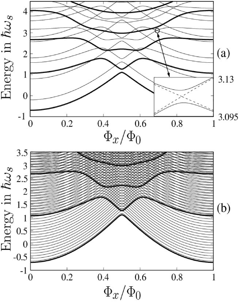
Figure 3: (a) Energy eigenvalues versus $\varphi_{x}$ of the SQUID ring Hamiltonian $H_{s}$ (thick lines) and the ring-field total Hamiltonian $H_{t}$ (thin lines) with $\omega_{e}=\omega_{s}$. The coupling constant $\mu=1/100$. The inset shows an example (arrowed) of the lifting of the degeneracy of the ring-field levels when $\mu\neq 0$. (b) as in figure(a) but with $\omega_{e}=\frac{1}{10}\omega_{s}$.

As an illustrative example we show in figures 3 the computed, $\varphi_{x}$ -dependent eigenvalues of $H_{t}^{\prime}$ for (a) $\omega_{e}=\omega_{s}$ (with truncations $N=\Sigma=5$) and (b) $\omega_{e}=\frac{1}{10}\omega_{s}$ (with truncations $N=50$ and $\Sigma=5$ ). In these figures the scaling is too small to reveal the lifting of the degeneracy at the crossing points by the nonzero coupling term $\left(\mu\neq 0\right)$. Again to illustrate, we show in the inset of figure 3(a), but at much higher resolution, one such computed crossing point. Here the splitting of the crossing energies is quite apparent, these being intimately connected to the functional form of the original SQUID ring eigenenergies. That such crossing points have been reported in experimental studies of Josephson weak link circuits, particularly SQUID rings, with concomitant superpositions of macroscopic states (Schrodinger cats), is further evidence for the underlying quantum mechanical nature of these systems S ; N ; L ; M . It is therefore timely to develop a full quantum treatment of SQUID ring-em field systems, which is the purpose of the paper.

In the above we have studied the eigenproblem ${{H_{t}^{\prime}}}\left|\xi_{n}\right\rangle=\Xi_{n}\left|\xi_{n}\right\rangle$ using a truncated basis. We use now these results to compute the evolution operator as

$$U\left(t\right)=\sum_{n}\left|\xi_{n}\right\rangle\exp\left(-\frac{i\Xi_{n}t}{\hbar}\right)\left\langle\xi_{n}\right|$$ (7)

Assuming that the system at $t=0$ is described by the density matrix $\rho(0)$, we have calculated the density matrix $\rho(t)=U(t)\rho(0)U^{\dagger}(t)$ at a later time $t$ and the reduced density matrices $\rho_{e}={\rm Tr}_{{s}}\left(\rho\right)$, $\rho_{s}={\rm Tr}_{{e}}\left(\rho\right)$. As a measure of the accuracy of the truncation approximation we have also calculated the traces of all the density matrices that we use. In the limit of infinite order density matrices the trace is equal to $1$, while for truncated density matrices it should be very close to $1$. In all our results the trace was greater than $0.99$. Another test we performed was to increase the cutoff point from which we were able to ascertain that our truncation had negligible effect.

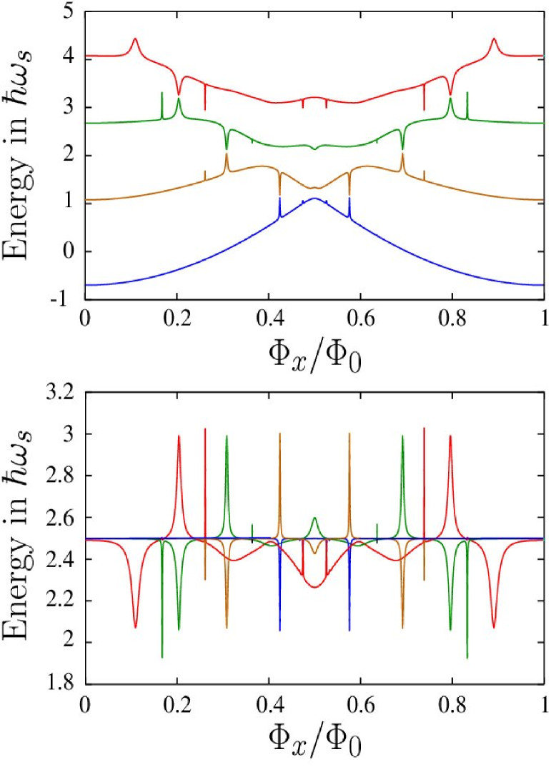
Figure 4: The time averaged energy levels versus $\varphi_{x}$ for (a) the ring ($\left\langle H_{s}\right\rangle$)and (b) the field ($\left\langle H_{e}\right\rangle$). The coupling constant $\mu=1/100$ and $\omega_{e}=\omega_{s}$. At $t=0$ the electromagnetic field is assumed to be in the coherent state $|\alpha=i\sqrt{2}\rangle$ and the ring in the energy eigenstates: $\sigma=0$ (blue), $\sigma=1$ (brown), $\sigma=2$ (green) and $\sigma=3$ (red).

Figure 5: The time averaged energy levels versus $\varphi_{x}$ for (a) the ring ($\left\langle H_{s}\right\rangle$)and (b) the field ($\left\langle H_{e}\right\rangle$). The coupling constant $\mu=1/100$ and $10\omega_{e}=\omega_{s}$. At $t=0$ the electromagnetic field is assumed to be in the coherent state $|\alpha=i10\sqrt{2}\rangle$ and the ring in the energy eigenstates: $\sigma=0$ (solid), $\sigma=1$ (dashed).

We define the time averaged energy expectation values $H{{{}^{\prime}}}_{{s}}$ and $H_{{e}}$ as $\left(i=s,e\right)$

$$\langle\langle H_{i}\rangle\rangle=\lim_{T\rightarrow\infty}\frac{1}{T}\int_{0}^{T}{\rm Tr}[\rho_{i}(t)H_{i}]\ dt$$ (8)

where, computationally, we integrate from $0$ up to $20,000/\omega_{s}$ which we have found to be sufficient to ensure the convergence of the integral (8) for all the results presented in this paper. In figure 4 we display the computed, time averaged, energy expectation values (normalized in units of $\hbar\omega_{s}$) of $H{{{}^{\prime}}}_{{s}}$ [figure 4(a)] and $H{{\ {}^{\prime}}}_{{e}}$ [figure 4(b)]. These have been calculated over the range $0\leq\varphi_{x}\leq 1$ for various values of $\sigma\left(=0,1,2,3\right)$, with $\mu=1/100$ and $\omega_{e}=\omega_{s}$. In computing these results we have set the $t=0$ state as $|\alpha=i\sqrt{2}\rangle_{e}\otimes|\sigma\rangle_{s}$, where $|\alpha\rangle_{e}$ is a coherent state of the em field ($a_{e}|\alpha\rangle_{e}=\alpha|\alpha\rangle_{e}$). As is apparent in figures 4(a) and (b), for specific values of external bias flux $\varphi_{x}$ [namely those corresponding to the crossing points shown in figure 3(a)] there is a strong interaction between the em field and the SQUID ring. As is also apparent, this leads to an energy exchange between the components of the system. To demonstrate how the time averaged energy levels for the ring and field depend on the ratio of $\omega_{s}$ to $\omega_{e}$, we show in figure 5(a) and (b), respectively, these levels computed for $\sigma=0,1$ and, again, $\mu=1/100$ but now $\omega_{e}=\omega_{s}/10$. In order for the energy of our initial state to be equal to that used in the previous example, here this state is chosen to be $|\alpha=i10\sqrt{2}\rangle_{e}\otimes|\sigma\rangle_{s}$. As is to be expected, starting with $\sigma=0,1$ eigenstates, the separation in $\varphi_{x}$ between the regions of strong coupling (energy exchange) are significantly reduced compared to those seen in figure 4. As a further example, we show in figure 6 the computed results for our coupled system taking, as in figure 4, $\omega_{e}=\omega_{s}$ but now with stronger coupling $\left(\mu=1/10\right)$. To make our results strictly comparable with those of figure 4, we use the initial state $|\alpha=i\sqrt{2}\rangle_{e}\otimes|\sigma=0\rangle_{s}$. Due to the stronger coupling we can see more regions in external bias flux where energy is exchanged between the two components of the system. In all three sets of results (figures 4, 5 and 6) there are peaks (both upwards and downwards) generated in the time averaged energies about specific values of $\varphi_{x}$. These peak regions, where energy is exchanged between the field and the ring, correspond to quantum transitions in the ring and in all cases demonstrate strong coupling between the two oscillators in the system.

Figure 6: The time averaged energy levels versus $\varphi_{x}$ for the ring ($\left\langle H_{s}\right\rangle$) and the field ($\left\langle H_{e}\right\rangle$). The coupling constant $\mu=1/10$ and $\omega_{e}=\omega_{s}$. At $t=0$ the electromagnetic field is assumed to be in the coherent state $|\alpha=i\sqrt{2}\rangle$ and the ring in the lowest eigenstate $\sigma=0$.

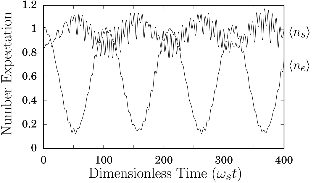
Figure 7: The expectation values $\left\langle n_{e}\right\rangle$ and $\left\langle n_{s}\right\rangle$ as functions of time for $\varphi_{x}=0.426,$ $\mu=1/10$ and $\omega_{e}=\omega_{s}$. At $t=0$ the electromagnetic field is assumed to be in the number state $|1\rangle$ and the ring is in the energy eigenstate $\sigma=0$.

To illustrate the quantum mechanical effects associated with this coupling we take as an example the case of $\mu=1/10$, $\omega_{e}=\omega_{s}$ (as in figure 6) and set $\varphi_{x}=0.426$ (arrowed in figure 6) at which flux bias the coupling (and the energy exchange) between the ring and field is strong. We assume that at $t=0$ the em field is in the number state $|1\rangle$ ($a_{e}^{\dagger}a_{e}|1\rangle_{e}=1|1\rangle_{e}$) and the ring is in the energy eigenstate $\sigma=0$ (we stress that $\sigma$ are eigenstates of $H_{s}$ and not of $n_{s}=a_{s}^{\dagger}a_{s}$ ). In figure 7, with these values of $\omega_{s}$, $\mu$ and $\varphi_{x}$, we show the computed expectation values of the photon number $\left\langle n_{e}\right\rangle={\rm Tr}(\rho_{e}a_{e}^{\dagger}a_{e})$ in the field, and $\left\langle n_{s}\right\rangle={\rm\ Tr}(\rho_{s}a_{s}^{\dagger}a_{s})$ in the ring, as functions of time. These results demonstrate that a strong exchange in energy takes place quasi-periodically in time between the ring and the field, i.e. when the photon number expectation value in the SQUID ring increases that in the em field decreases, and vice versa. We note that in order to compare these predictions with experiment we would need to to measure the actual power level of the em field. We also note that with the ring-field coupling constant known this would allow us to estimate the em power impinging on the SQUID ring.

As the system evolves in time its two components-oscillator mode and SQUID ring - become entangled quantum mechanically. In order to quantify this entanglement we use entropic quantities. For a two mode (field-ring) system $e-s$ this entanglement can be quantified according to the expression lin73 ; lieb75 ; wehrl78 ; barnett91

$$I_{es}=S\left(\rho_{e}\right)+S\left(\rho_{s}\right)-S\left(\rho\right)$$ (9)

where $S\left(\rho\right)$ is the von-Neumann entropy given by

$$S\left(\rho\right)=-{\rm Tr}\left[\rho\ln\left(\rho\right)\right]$$ (10)

Figure 8: The entropies as a function of time for the same system as in figure 7.

and the entanglement entropy is positive or zero (subadditivity property of the entropy). In figure 8 we show the time dependent computed entropies $S\left(\rho_{e}\right)$, $S\left(\rho_{s}\right)$, and the entanglement entropy $I$, for the same system as in figure 7. From these results it is quite apparent that although at $t=0$ both the field and the ring are in a pure state, they both evolve into mixed states. Of course, since the time evolution is unitary the joint field-ring system is always in a pure state $\left(S(\rho)=0\right)$. The results presented in figure 8 do demonstrate that the system does become highly entangled over time although, as can be seen, at certain times it can disentangle again. There is no doubt that for the development of truly quantum technologies, for example, quantum computing and quantum communications, such states of entanglement are of great importance. We note in particular, that in some of these schemes the ability of the system to control the entanglement (as in our case) is highly desirable. In principle, experimental verification of the entanglement between the two modes could be achieved through Bell type of inequalities. However, in the context of the present work their exact form will require further investigation.

III A SQUID ring coupled to a classical em field

In previous work we treated the em field classically 3. and used the Hamiltonian

$$H_{s}=\frac{Q_{s}^{2}}{2C_{s}}+\frac{\left(\Phi_{s}-\left[\Phi_{x}+\varphi_{e}\sin(\omega_{e}t)\right]\right)^{2}}{2\Lambda_{s}}-\hbar\nu\cos\left(2\pi\frac{\Phi_{s}}{\Phi_{0}}\right).$$ (11)

and solved the corresponding time-dependent Schrödinger equation. Here $\varphi_{e}$ is taken to be the magnetic flux amplitude of the classical em field. It is of interest to compare the quasi-classical results derived via (11) with the fully quantum results found above where the initial state of the em field is a coherent state. Due to the quasi-classical nature of the coherent state we expect some agreement between the fully quantum results and the quasi-classical results. To furnish an example to compare with these quantum results, we have computed the time averaged ring energy expectation values for the Floquet states (eigenvalues of the evolution operator after one period of microwave evolution) as a function of $\varphi_{x}$ using the same value of microwave field amplitude $\left(\varphi_{e}=0.41\mu\Phi_{0}\right)$ as in figure 4(a). Our results are presented in figure 9. Within the computational accuracy available, and given that we are dealing with two different regimes of the coupled system, it is clear that the principal transition region features match in both models, even though the amplitudes may not be the same.

Figure 9: Time-dependent Schrödinger equation (Eq 12) calculation of the time averaged ring energy levels against $\Phi_{x}$ with $\mu=1/100$ , $\omega_{e}=\omega_{s}$ and $\varphi_{e}=0.41\mu\Phi_{0}$ Here the electromagnetic field is treated classically and the time-dependent Schrödinger equation (12) is solved. The results of this figure should be compared and contrasted with those of figure 4a.

IV Discussion

We have studied the coupling of a SQUID ring to a single mode em field at frequencies in the sub-THz to THz range where, in general, $k_{B}T<\hbar\omega_{s},\hbar\omega_{e}$ so that the system behaves quantum mechanically. In this we have been strongly influenced by recent discussions in the literature on routes to quantum computing using Josephson devices1. ; 2. ; schon1999 ; A and on even more recent publication of experimental data on superposition states in SQUID rings L ; M . In the paper we have shown that our results [for example, figure 4(a)] compare well with previous semi-classical (Floquet method) computations made by us (figure 9 and ref 11) and have expanded this work to calculate explicitly the photon number and entanglement states in the coupled ring-field system. We note the relation between the results presented in this paper and previous work on em environments in thermal equilibrium with Josephson (e.g. SQUID) circuits  dev90 ; girvin90 ; averin90 ; flen91 ; ingold91 ; falci91 ; maas91 . In our work we have assumed that the external em field is in a particular quantum state and our results depend on this state. As an example we have considered the em field at $t=0$ to be in a coherent state. However, the calculations can easily be repeated for another initial state of the field. Each initial state will, of course, yield different results.

In addition to the em field a magnetostatic flux also threads the SQUID ring. In this paper we have demonstrated that for certain values of this flux strong coupling develops at which point(s) large amounts of energy are exchanged between the ring and the field. Future experimental probing of these energy exchanges, which is considered again in the discussion section, would clearly be of great interest. We have also demonstrated that entanglement between the ring and field modes arises as a natural consequence of the full quantum mechanics of the system. As we have pointed out (section II, above), experimental verification of such entanglements will require further work on the Bell inequalities related to these entanglements.

In our calculations we have neglected dissipation and have calculated the time evolution of the system using the equation $\partial_{t}\rho=-\left(i/\hbar\right)[H,\rho]$. A more realistic calculation to take into account dissipation due to the external environment Leg can be made with the equation $\partial_{t}\rho=-\left(i/\hbar\right)[H,\rho]+f(\rho)$ where the $f(\rho)$ are dissipative terms. Numerical work to include these terms is currently in progress.

Of general interest to experimentalists working on (time dependent) superposition states in SQUID ring devices is the problem of determining the actual em power (or number of photons in each state of the em field) coupled to the ring. Together with the frequency of the em field, and the original eigenenergies of the ring, this is required in order to compute the ring crossing point splittings. In principle, this problem can be overcome through the kind of analysis we have undertaken in this paper, whether it be for classical em fields3. or photon states interacting with a quantum mechanical SQUID ring. As we have shown, it is possible to determine these power levels accurately through following the reactive frequency shift of a SQUID ring-classical (radio frequency) resonator system, driven by an external em field, when the ring remains adiabatically in its quantum mechanical ground state. However, where em frequencies and/or amplitudes are high enough (as in this paper), so that (time dependent) superpositions of low lying energy eigenstates of the ring are generated, the problem becomes very much more difficult theoretically. Nevertheless, there appear to be several routes to resolving these difficulties, as indicated by some of our recent investigations of non-adiabatic processes in em-driven SQUID rings  whiteman1997 ; thesis . We note that at sufficiently high em frequencies/amplitudes multiphoton absorption and emission processes will occur between the components of the coupled system. This may complicate the interpretation of experimental data and will be a topic of further theoretical investigation by us. For the future, we also note that it may be possible to extend these experimental and theoretical techniques to probe the details of energy exchange and entanglement of the system presented in this paper.

There now exists a clearly defined need to create THz technology pep00 for a range of applications including modern communications. To date this technology, based on quantum processes on the small scale, functions classically at the device level. A primary purpose of this paper has been to demonstrate that at THz frequencies, and reasonable operating temperatures $\left(\char 126\relax 4K\right)$, this technology could be made fully quantum mechanical in nature, i.e. at high enough SQUID ring and em oscillator frequencies both can be treated as macroscopic quantum objects, irrespective of any deeper description of the superconducting condensate in SQUID rings  ralph1996 ; ralph1997 . This would point to a great richness of potential applications. For example, in the context of the results presented here, our investigations may prove useful for the development of frequency converters up to THz frequencies and beyond. More generally these results, and the theoretical descriptions underlying them, may find use in the emerging fields of quantum technology and quantum computation 1. ; 2. ; schon1999 ; A .

- (1) See, for example,“Introduction to Quantum Computation and Information”, eds. H.K. Lo, S. Popescu and T.P. Spiller (World Scientific, New Jersey, 1998).
- (2) T.P. Orlando, J.E. Mooij, L. Tian, C.H. van der Wal, L.S. Levitov, S. Lloyd and J.J. Mazo, Phys. Rev. B. 60, 15398 (1999).
- (3) Y. Makhlin, G. Schön and A. Shnirman, Nature. 398, 305 (1999).
- (4) D. Averin Nature 398, 748 (1999)
- (5) R. Rouse, S. Han, J.E. Lukens, Phys. Rev. Lett. 75, 1614 (1995)
- (6) P.Silvestrini, B.B. Ruggierio, C. Granata, E. Esposito, Phys. Lett. A 267, 45 (2000)
- (7) Y. Nakamura, C.D. Chen, J.S. Tsai, Phys. Rev. Lett 79, 2328 (1997)
- (8) Y. Nakamura, Y.A. Pashkin, J.S. Tsai, Nature 398, 786 (1999)
- (9) J.R. Friedman, V. Patel, W. Chen, S.K. Tolpygo, J.E. Lukens, Nature 406, 43 (2000)
- (10) C.H. van der Wal, A.C.J. ter Haar, F.K. Wilhem, R.N. Schouten, C.J.P.M. Harmans, T.P. Orlando, S. Lloyd, J.E. Mooij, Science 290, 773 (2000)
- (11) T.D. Clark, J. Diggins, J.F. Ralph, M.J. Everitt, R.J. Prance, H. Prance, R. Whiteman, A. Widom, and Y.N. Srivastava, Annals Phys. 268 , 1 (1998).
- (12) R. Whiteman, V. Schöllmann, M.J. Everitt, T.D. Clark, R.J. Prance, H. Prance, J. Diggins, G. Buckling, and J.F. Ralph, J. Phys. Condens. Matter 10, 9951 (1998).
- (13) R. Whiteman, T.D. Clark, R.J. Prance, H. Prance, V. Schöllmann, J.F. Ralph, and M.J. Everitt, J. Mod. Opt. 45, 1175 (1998).
- (14) G. Schon and A. D. Zaikin Phys. Rep., 198, 237 (1990)
- (15) Y. Makhlin, G. Schon and A. Shnirman, cond-mat/0011269
- (16) M. A. Kastner, Rev. Mod. Phys., 64, 849, (1992)
- (17) T. P. Spiller, T. D. Clark, R. J. Prance and A. Widom, Prog. Low Temp. Phys., 13, 219 (1992)
- (18) H.Grabert, M.H.Devoret (Editors) ‘Single-charge tunneling’ NATO ASI series Vol 294 (Plenum, NY,1992)
- (19) K.Wodkiewicz and J. H. Eberly, J. Opt. Soc. Am. B2, 458 (1985)
- (20) B. Yurke and S. L. McCall and J.R. Klauder Phys. Rev. A33, 4033 (1986)
- (21) R. A Campos, B.E.A Saleh and M. C. Teich, Phys. Rev. A40, 1371 (1989)
- (22) H. Fearn and R. Loudon. J. Opt. Soc. Am. B6, 971 (1989)
- (23) F. Singer R. A. Campos M. C. Teich and B. E. A. Saleh, Quant. Opt. 2, 307 (1990)
- (24) A. Vourdas, Phys. Rev. A46, 442 (1992)
- (25) G. Lindbland, Commun. Math. Phys. 33, 305, (1973)
- (26) E. H. Lieb Bull. Am. Math. Soc. 81, 1 (1975)
- (27) A. Wehrl, Rev. Mod. Phys. 50, 221 (1978)
- (28) S. M. Barnett and S. J. D. Phoenix, Phys. Rev. A44, 535 (1991)
- (29) M.H. Devoret, D. Esteve, H. Grabert, G.L. Ingold, H. Pothier, C. Urbina Phys. Rev. Lett. 64, 1824 (1990)
- (30) S.M. Girvin, L.I. Glazman, M. Jonson, D.R. Penn, M.D. Stiles Phys. Rev. Lett. 64, 3183 (1990)
- (31) D.V. Averin, Yu.V. Nazarov, A.A. Odintsov, Physica B165/166, 945 (1990)
- (32) K. Flensberg, S.M. Girvin, M. Jonson, D.R. Penn, M.D. Stiles Z. Phys. B85, 395 (1991)
- (33) G.L. Ingold, P. Wyrowski, H. Grabert, Z. Phys. B85 , 443 (1991)
- (34) G. Falci, V. Bubanja, G. Schon, Z. Phys. B85, 451 (1991)
- (35) A. Maassen van den Brink, A.A. Odintsov, P.A. Bobbert, G. Schon, Z. Phys. B85, 459 (1991)
- (36) A.J. Leggett et al, Rev. Mod. Phys. 59 1 (1987)
- (37) R. Whiteman, T.D. Clark, R.J. Prance, H. Prance, V. Schöllmann, J.F. Ralph, M. Everitt and J. Diggins. J. Mod. Optics 45 , 1175 (1998).
- (38) M.J. Everitt, ”Quantum Dynamics and Measurment of Single Quantum Objects”, DPhil Thesis, University of Sussex (February, 2000).
- (39) See, for example, D.D. Amone, C.M. Ciesla and M. Pepper, TeraHertz imaging comes into view, Physics World 13(4), 35-40 (April 2000); J. Faist, F. Capasso, D.L. Sivco, C. Sirtori, A.L. Hutchinson, A.Y. Cho, Quantum Cascade Laser, Science 264: (5158) 553-556 (April 1994).
- (40) J.F. Ralph, T.D. Clark, R.J. Prance and H. Prance. Physica B 226, 355 (1996).
- (41) J.F. Ralph, T.D. Clark, J. Diggins, R.J. Prance, H. Prance and A. Widom. J. Phys.: Condens Matter 9, 8275 (1997).