Vortex motion in a finite–size easy–plane ferromagnet and application to a nanodot

Abstract

We study the motion of a non–planar vortex in a circular easy–plane ferromagnet, which imitates a magnetic nanodot. Analysis was done using numerical simulations and a new collective variable theory which includes the coupling of Goldstone–like mode with the vortex center. Without magnetic field the vortex follows a spiral orbit which we calculate. When a rotating in–plane magnetic field is included, the vortex tends to a stable limit cycle which exists in a significant range of field amplitude $B$ and frequency $\omega$ for a given system size $L$. For a fixed $\omega$, the radius $R$ of the orbital motion is proportional to $L$ while the orbital frequency $\Omega$ varies as $1/L$ and is significantly smaller than $\omega$. Since the limit cycle is caused by the interplay between the magnetization and the vortex motion, the internal mode is essential in the collective variable theory which then gives the correct estimate and dependency for the orbit radius $R\sim BL/\omega$. Using this simple theory we indicate how an ac magnetic field can be used to control vortices observed in real magnetic nanodots.

I Introduction

Nonlinear topological excitations in 2D spin systems of soliton or vortex type are known to play an essential role in 2D magnetism. For example, solitons break the long–range order in 2D isotropic magnets. Vortices play a similar role in 2D easy–plane magnets. Magnetic vortices have been studied since the 1980s. They are important for the dynamical and thermodynamical properties of magnets, for a review see Ref. Mertens and Bishop, 2000. The vortex contribution to the response functions of 2D magnets has been predicted theoreticallyMertens et al. (1989) and observed experimentallyWiesler et al. (1989).

A second wind in the physics of magnetic vortices appeared less than five years ago due to the direct observation of vortices in permalloy (Py, $\mathrm{Ni}_{80}\mathrm{Fe}_{20}$) Shinjo et al. (2000); Cowburn et al. (1998, 1999); Pulwey et al. (2001); Gubbiotti et al. (2002); Park et al. (2003) and $\mathrm{Co}$ Fernandez and Cerjan (2000); Raabe et al. (2000); Lebib et al. (2001) magnetic nanodots. Such nanodots are submicron disk–shaped particles, which have a single vortex in the ground state due to the competition between exchange and magnetic dipole–dipole interaction.Hubert and Schäfer (1998) A vortex state is obtained in nanodots that are larger than a single domain whose size is a few nanometers (e.g. for the Py–nanodot the exchange length $l_{\text{ex}}=5.9\,nm$). The vortex state of magnetic nanodots has drawn much attention because it could be used for high-density magnetic storage and miniature sensors. Cowburn (2002); Skomski (2003). For this one needs to control magnetization reversal, a process where vortices play a big role Guslienko et al. (2001). The vortex signature has been probed by Lorentz transmission electron microscopyRaabe et al. (2000); Schneider et al. (2002) and magnetic force measurementsPokhil et al. (2000); Fernandez and Cerjan (2000). Great progress has been made recently with the possibility to observe high frequency dynamical properties of the vortex state magnetic dots by Brillouin light scattering of spin waves Demokritov et al. (2001); Hillebrands and Ounadjela (2002), time–resolved Kerr microscopy Park et al. (2003), phase sensitive Fourier transformation technique Buess et al. (2004), and X–ray imaging technique Choe et al. (2004). These have shown that the vortex performs a gyrotropic precession when it is initially displaced from the center of the dot, e.g. by an in–plane magnetic field pulse. Usov and Kurkina (2002); Guslienko et al. (2002a); Park et al. (2003)

In general the vortex mesoscopic dynamics is described by the Thiele collective coordinate approach Thiele (1973, 1974); Huber (1982); Nikiforov and Sonin (1983), which considers the vortex as a rigid structure not having internal degrees of freedom.Mertens and Bishop (2000) However recent experimental and theoretical studies Ivanov et al. (1998); Gaididei et al. (2000); Raabe et al. (2000); Pulwey et al. (2001); Kovalev and Prilepsky (2002, 2003); Zagorodny et al. (2003); Kovalev et al. (2003) indicate phenomena which can not be explained using such a simple picture. One striking example is the switching of the vortex polarization Gaididei et al. (2000); Raabe et al. (2000); Pulwey et al. (2001); Kovalev and Prilepsky (2002, 2003); Zagorodny et al. (2003), where coupling occurs between the vortex motion and oscillations of its core. Another one is the cycloidal oscillations of the vortex around its mean path Ivanov et al. (1998); Kovalev et al. (2003) where the dynamics of the vortex center is strongly coupled to spin waves. In this way the internal dynamics of the vortex plays a vital part. One of the first attempts to take into account the internal structure of vortices was presented in Ref. Caputo et al., 2003 which showed that a variation of the core radius slaved to the position explained the motion of a vortex pair across an interface between two materials of different anisotropy. Some progress has been achieved in Ref. Zagorodny et al., 2004 where we have confirmed that internal degrees of freedom play a crucial role in the dynamics of vortices driven by an external time-dependent magnetic field in a classical spin system.

Here we present a complete study of this problem using direct numerical simulations of the spin system and a collective variable theory which includes an internal mode. We show that the periodic forcing of the system by the time dependent magnetic field together with the damping stabilizes the vortex in a finite domain. This limit cycle exists because of the interplay between the magnetization and the vortex position so that it is essential to include an internal mode in the collective variable theory to describe it. When this is done, the theory yields the domain of stability in parameter space and the main dependencies on the field amplitude $B$ and frequency $\omega$. It can be seen as a one of the first generalizations to vortices of the collective variable theories developed for 1D Klein-Gordon kinks by Rice Rice (1983); Quintero et al. (2000a, b) which include the width of the kink together with its position.

In the next section II we formulate the continuum model, discuss the role of different types of interactions and briefly review the main results on the structure of the vortex solution. The vortex motion without external field is examined in section III. It follows a spiral orbit as a result of the competition between the gyroforce, the Coulomb force and the damping force. In section IV with the ac driving, numerical simulations show that the vortex converges to a stable limit cycle. We give its boundaries in parameter space and indicate how the radius and frequency of the vortex orbital motion depends on the field and geometry parameters. Section V presents and discusses in detail the new collective variable theory of the observed vortex dynamics which takes into account the coupling between an internal shape mode and the translational motion of the vortex position. In section VI we link this with the individual spin motion observed in the simulations and indicate how these effects can be observed and used in real nano magnets.

The model we consider is a ferromagnetic system with spatially homogeneous uniaxial anisotropy, described by the classical Heisenberg Hamiltonian

$$\begin{split}\mathscr{H}_{0}=&-\frac{J}{2}\!\!\sum_{\left(\bm{n},\bm{n}^{\prime}\right)}\!\left(\bm{S}_{\bm{n}}\cdot\bm{S}_{\bm{n}^{\prime}}-\delta S^{z}_{\bm{n}}S^{z}_{\bm{n}^{\prime}}\right)+\frac{K}{2}\!\!\sum_{\bm{n}}\left(S^{z}_{\bm{n}}\right)^{2}\!\!.\end{split}$$ (1)

Here $\bm{S}_{\bm{n}}\equiv\left(S^{x}_{\bm{n}},S^{y}_{\bm{n}},S^{z}_{\bm{n}}\right)$ is a classical spin vector with fixed length $S$ on the site $\bm{n}$ of a two-dimensional square lattice, and the exchange integral $J>0$ for a ferromagnet. The first summation runs over nearest–neighbor pairs $(\bm{n},\bm{n}^{\prime})$. We assume a small anisotropy leading to an easy-plane ground state. This anisotropy can be either of the exchange type, with $0<\delta\ll 1$, or of the on–site type, with $0\leq K\ll J$.

Extending ideas of Ref. Zagorodny et al., 2004 we study the movement of a vortex in this system under the action of a magnetic field $\bm{B}(t)=\left(B\cos\omega t,B\sin\omega t,0\right)$, which is spatially homogeneous and is rotating in the plane of the lattice. This field adds an interaction of the form

$$\mathscr{V}(t)=-\gamma B\sum_{\bm{n}}\left(S_{\bm{n}}^{x}\cos\omega t+S_{\bm{n}}^{y}\sin\omega t\right),$$ (2)

where $\gamma=2\mu_{B}/\hslash$ is the gyromagnetic ratio.

The spin dynamics is described by the Landau–Lifshitz equations with Gilbert damping

$$\frac{d\bm{S}_{\bm{n}}}{dt}=-\left[\bm{S}_{\bm{n}}\times\frac{\partial\mathscr{H}}{\partial\bm{S}_{\bm{n}}}\right]-\frac{\varepsilon}{S}\left[\bm{S}_{\bm{n}}\times\frac{d\bm{S}_{\bm{n}}}{dt}\right],$$ (3)

where $\mathscr{H}=\mathscr{H}_{0}+\mathscr{V}(t)$ is the total Hamiltonian. Eqs. (3) preserve the length of the spins $|\bm{S}_{\bm{n}}|\equiv S$, which has units of action. Another form of Eqs. (3) more suitable for spin dynamics simulations is given in Appendix A.

II Continuum Limit

In the case of weak anisotropies $\delta\ll 1$, $K\ll J$, the characteristic size of excitations $l_{0}=a\sqrt{{J}/({4J\delta+K})}$ is larger than the lattice constant $a$, so that in the lowest approximation on the small parameter $a/l_{0}$ and weak gradients of magnetization we can use the continuum approximation for the Hamiltonian (1)

$$H_{0}\equiv\mathscr{H}_{0}-E_{0}=\frac{JS^{2}}{2}\int d^{2}x\left[\left(\nabla\bm{s}\right)^{2}+\frac{m^{2}}{l_{0}^{2}}\right],$$ (4)

where $E_{0}$ is a constant. The spin length has been rescaled so that

$$\bm{s}=\bm{S}/S=\left(\sqrt{1-m^{2}}\cos\phi;\sqrt{1-m^{2}}\sin\phi;m\right)$$ (5)

is a unit vector. The length $l_{0}$ coincides with the radius of the vortex core obtained in Ref. Nikiforov and Sonin, 1983 for on-site anisotropy type alone ($\delta=0$). For the case of exchange anisotropy alone ($K=0$), it is also customary to use the length $r_{\text{v}}=a\sqrt{(1-\delta)/4\delta},$ which is obtained from an asymptotic analysis and is to be identified later with the radius of the “core” of a vortex.Gouvêa et al. (1989); Mertens et al. (1997) However, for the range of $\delta$ we are interested in, i.e. for $\delta\lesssim 0.1$, the difference between $r_{\text{v}}$ and $l_{0}$ is negligible.

The interaction with a homogeneous time-dependent magnetic field is expressed as

$$\begin{split}V(t)&=-\frac{JS^{2}}{l_{0}^{2}}\,\int\,d^{2}x\left(\bm{b}(t)\cdot\bm{s}(\bm{r},t)\right)\\ &=-JS^{2}b\int\,\,d^{2}\xi\,\,\sqrt{1-m^{2}}\cos\left(\phi-\nu\tau\right).\end{split}$$ (6)

In order to simplify notations we use here and below the dimensionless coordinate $\bm{\xi}\equiv\bm{r}/l_{0}$, the dimensionless time $\tau\equiv\omega_{0}t$, the dimensionless driving frequency $\nu=\omega/\omega_{0}$ and the dimensionless magnetic field $\bm{b}=\gamma\bm{B}/\omega_{0}$,Ivanov and Sheka (1995); Ivanov and Wysin (2002) where

$$\omega_{0}=S\left(4J\delta+K\right).$$ (7)

In all real magnets there is, in addition to short–ranged interactions, a long–ranged dipole–dipole interaction. In the continuum limit this interaction can be taken into account as energy of an effective demagnetization field, $\bm{H}^{(m)}$

$$\mathscr{E}^{(m)}=-\int\!d^{2}x\ \bm{M}\cdot\bm{H}^{(m)},$$

where $\bm{M}$ is the magnetization. Generally, this field is a complicated functional of $\bm{M}$. However, in the case of a thin magnetic film (or particle) the volume contribution to the demagnetization field is negligible, and only surface fields are important. The face surfaces produce a local field $\bm{H}^{(m)}=-4\pi M_{0}\bm{e}_{z}$ for the sample with the saturation magnetization $M_{0}$. Then the dipole–dipole interaction can be taken into account by a simple redefinition of the anisotropy constants, $K\to K^{\text{eff}}=K+4\pi M_{0}^{2}a^{2}/S^{2}$, leading to a new magnetic length Ivanov and Yastremsky (2001)

$$l_{0}\to l_{0}^{\text{eff}}=a\sqrt{\frac{J}{4J\delta+K+4\pi M_{0}^{2}a^{2}/S^{2}}}.$$ (8)

This is the case of so–called configurational or shape anisotropy. Schabes and Bertram (1988); Cowburn et al. (1998); Cowburn (2002) The lateral surface affects only the boundary conditions, see Refs. Guslienko et al., 2002b; Ivanov and Zaspel, 2002 for details. For example, for a very thin magnetic particle, which corresponds to our 2D system, free boundary conditions are valid, and we will use them in the paper.

Thus, the total energy functional, normalized by $JS^{2}$, reads

$$\mathscr{E}[\bm{s}]=\int d^{2}\xi\left[\frac{\left(\nabla\bm{s}\right)^{2}}{2}+\frac{m^{2}}{2}-\left(\bm{b}\cdot\bm{s}\right)\right],$$ (9)

where we have rescaled the magnetic length in accordance with (8).

The continuum version of the Landau–Lifshitz Eqs. (3) becomes

$$\frac{\partial\phi}{\partial\tau} =\frac{\delta\mathscr{E}}{\delta m}+\frac{\varepsilon}{(1-m^{2})}\frac{\partial m}{\partial\tau},$$ (10a)

$$\frac{\partial m}{\partial\tau} =-\frac{\delta\mathscr{E}}{\delta\phi}-\varepsilon(1-m^{2})\frac{\partial\phi}{\partial\tau}.$$ (10b)

These equations can be derived from the Lagrangian

$$\mathscr{L}=-\int d^{2}\xi(1-m)\frac{\partial\phi}{\partial\tau}-\mathscr{E}[\bm{s}]$$ (11)

and the dissipation function

$$\mathscr{F} =\frac{\varepsilon}{2}\int d^{2}\xi\left(\frac{\partial\bm{s}}{\partial\tau}\right)^{2}$$ (12)

$$=\frac{\varepsilon}{2}\int d^{2}\xi\left[\frac{1}{1-m^{2}}\left(\frac{\partial m}{\partial\tau}\right)^{2}+(1-m^{2})\left(\frac{\partial\phi}{\partial\tau}\right)^{2}\right].$$

Then Eqs. (10) result explicitly in

$$\frac{\partial\phi}{\partial\tau} =-\frac{m\,\left(\bm{\nabla}m\right)^{2}}{(1-m^{2})^{2}}+m\left[1-\left(\bm{\nabla}\phi\right)^{2}\right]-\frac{\Delta m}{1-m^{2}}$$

$$+\frac{b\,m\,\cos(\phi-\nu\tau)}{\sqrt{1-m^{2}}}+\frac{\varepsilon}{(1-m^{2})}\,\frac{\partial m}{\partial\tau},$$ (13a)

$$\frac{\partial m}{\partial\tau} =\bm{\nabla}[(1-m^{2})\bm{\nabla}\phi]-b\sqrt{1-m^{2}}\sin(\phi-\nu\tau)$$

$$-\varepsilon(1-m^{2})\frac{\partial\phi}{\partial\tau}.$$ (13b)

Without magnetic field the ground state of the system is a uniform planar state $m=0$ and $\phi=\text{const}$. The field changes essentially the picture: spins start to precess homogeneously in the XY–plane, $\phi=\varphi+\nu\tau$. Such a precession causes the appearance of a z–component of magnetization, $m=\text{const}$. From Eqs. (13), we find that the equilibrium values of $m$ and $\phi$ satisfy the following equations,

$$\left(1-\frac{\nu}{m}\right)^{2}+\varepsilon^{2}\nu^{2}=\frac{b^{2}}{1-m^{2}},$$ (14a)

$$-b\sin\phi-\varepsilon\nu\sqrt{1-m^{2}}=0,$$ (14b)

so that this state can only exist if $b\geq\varepsilon\nu$ (otherwise only the ground state with $m=0$ and $\phi=\text{const}$ exists). Assuming $m\ll 1$, we obtain

$$m\approx\frac{\nu}{1-\sqrt{b^{2}-\varepsilon^{2}\nu^{2}}},\quad\phi=\nu\tau+\pi+\arcsin\frac{\varepsilon\nu\sqrt{1-m^{2}}}{b}.$$ (15)

Note how the magnetization $m$ is proportional to the field frequency $\nu$ so that its sign is important. Below we discuss the role of this homogeneous solution in the vortex dynamics.

The continuum analogue of the power–dissipation relation (49) for the total energy functional $\mathscr{E}[\bm{s}]$ is calculated from Eqs. (11), (12) and gives

$$\frac{d\mathscr{E}}{d\tau}=-2\mathscr{F}-\mathscr{W},\qquad\mathscr{W}=\int d^{2}\xi\left(\bm{s}\cdot\frac{d\bm{b}}{d\tau}\right).$$ (16)

Formally, Eqs. (14) have two solutions. One can check that only for the solution (15) the dissipation balances the work done by the field, so that the energy $\mathscr{E}$ tends to be stabilized.

Static Vortices

The simplest nonlinear excitation of the system is the well–known non–planar magnetic vortex. We recall briefly the structure of a single static vortex at zero field. In this case the pair of functions $(m,\phi)$ satisfies the Eqs. (10) with the time derivatives set to zero and $b=0$. If we look for planar solutions ($m=0$) for the $\phi$ field, Eq. (10b) becomes the Laplace equation. For the vortex solution located at $Z=X+iY=R\exp(i\Phi)$ the $\phi$–field has the form:

$$\phi(z)=\varphi_{0}+q\arg\left(z-Z\right),$$ (17)

where $z=x+iy$ is a point of the XY–plane, $q\in\mathbb{Z}$ is the $\pi_{1}$ topological charge of the vortex (vorticity). We will call the solution with $q=1$ a vortex and the solution with $q=-1$ an antivortex. The expression (17) does not satisfy the boundary conditions for a finite system. For our circular system of radius $L$ (in units of $l_{0}$) and free boundary conditions the solution is Kovalev et al. (2003)

$$\phi=\arg\left(z-Z\right)-\arg\left(z-Z_{I}\right)+\arg Z,$$ (18)

where the “image” vortex is added at $Z_{I}=ZL^{2}/R^{2}$ to satisfy the Neuman boundary conditions. The last term in (18) is inserted to have the correct limit for $L\rightarrow\infty$.

The $m$–field has radial symmetry, $m\equiv\cos\theta\left({\rho}\equiv|z-Z|\right)$. From (13) and (17) one can derive that $\theta(\bullet)$ satisfies the following differential problem:

$$\frac{d^{2}\theta}{d{\rho}^{2}}+\frac{1}{\rho}\frac{d\theta}{d{\rho}}+\sin\theta\cos\theta\left(1-\frac{1}{{\rho}^{2}}\right)=0,$$ (19a)

$$\cos\theta(0)=p,\qquad\cos\theta(\infty)=0,$$ (19b)

where $p=\pm 1$ is the so–called polarity of the vortex. The solution of this differential problem is a bell–shaped structure with a width in the order of $l_{0}$.

III Vortex motion at zero field

A standard description for the steady movement of magnetic excitations was given first by Thiele. Thiele (1973, 1974) Huber Huber (1982), Nikiforov and Sonin Nikiforov and Sonin (1983) have first applied this approach to the dynamics of magnetic vortices, using a traveling wave Ansatz $\bm{s}(z,\tau)=\bm{s}\left(z-Z(\tau)\right)$. In terms of the fields $m$ and $\phi$ such an Ansatz is

$$m(z,\tau) =\cos\theta\left(|z-Z(\tau)|\right),$$ (20a)

$$\phi(z,\tau) =\arg\left(z-Z(\tau)\right)-\arg\left(z-Z_{I}(\tau)\right)+\arg Z(\tau),$$ (20b)

where the function $\theta(\bullet)$ describes the out–of–plane structure of the static vortex, and is the solution of Eqs. (19).

To derive an effective equation of the vortex motion for the collective variable $\bm{R}(\tau)=\left(X(\tau),Y(\tau)\right)$, we project the Landau–Lifshitz Eqs. (10) over the lattice using Ansatz (20). We obtain a Thiele equation in the form of a force balance,Mertens and Bishop (2000)

$$G\left[\bm{e}_{z}\times\dot{\bm{R}}\right]-2\pi\eta\dot{\bm{R}}+\bm{F}=0,$$ (21)

where the dot indicates derivative with respect to the rescaled time $\tau$. The first term, the gyroscopic force, acts on the moving vortex and determines the main properties of the vortex dynamics. The value of the gyroconstant is well–known $G=2\pi pq$, Huber (1982); Nikiforov and Sonin (1983) in our case for the vortex with positive polarity and unit vorticity $G=2\pi$. The second term describes the damping force with a coefficient Huber (1982); Kamppeter et al. (1999)

$$\eta={1\over 2}\varepsilon(\ln{L}+C_{1}),$$ (22)

where $C_{1}\approx 2.31$ is a constant coming from the $m$ field and is calculated in the appendix, see formula (62). The $\ln{L}$ dependence in $\eta$ was obtained in Ref. Huber, 1982.

The last term in Eq. (21) is an external force, acting on the vortex, $\bm{F}=-\bm{\nabla}_{\!\!\bm{R}}\mathscr{E}$, where $\mathscr{E}$ is the total energy functional (9). Without magnetic field ($\bm{b}=0$) such a force appears as a result of boundary conditions, it describes the 2D Coulomb interaction between the vortex and its image

$$\mathscr{E}^{\text{int}}=\mathscr{E}_{0}+\pi\ln\frac{L^{2}-R^{2}}{L},$$ (23)

where $\mathscr{E}_{0}\approx\pi$ is the energy of the vortex core.Kovalev et al. (2003)

In order to generalize the effective equations of the vortex motion for the case of the magnetic field we derive now the same effective equations by the effective Lagrangian technique as it was proposed in Refs. Zagorodny et al., 2003; Caputo et al., 2003; Zagorodny et al., 2004. Inserting Ansatz (20) into the “microscopic” Lagrangian (11) and the dissipative function (12), and calculating the integrals, we derive an effective Lagrangian (see Appendix B for the details)

$$\mathscr{L}=-\pi R^{2}\dot{\Phi}-\mathscr{E}^{\text{int}}.$$ (24)

In the same way we derive the effective dissipative function

$$\mathscr{F}=\pi\eta\dot{\bm{R}}^{2}=\pi\eta\left(\dot{R}^{2}+R^{2}\dot{\Phi}^{2}\right).$$ (25)

The equations of motion are then obtained from the Euler–Lagrange equations

$$\frac{\partial\mathscr{L}}{\partial X_{i}}-\frac{d\phantom{t}}{d\tau}\left(\frac{\partial\mathscr{L}}{\partial\dot{X}_{i}}\right)=\frac{\partial\mathscr{F}}{\partial\dot{X}_{i}}$$ (26)

for the $X_{i}=\left\{R,\Phi\right\}$,

$$\dot{\Phi}+\eta\frac{\dot{R}}{R}=\frac{1}{L^{2}-R^{2}},$$ (27a)

$$\frac{\dot{R}}{R}=\eta\dot{\Phi}.$$ (27b)

This set of equations is equivalent to the Thiele Eq. (21), when going to polar coordinates.

For zero damping ($\varepsilon=0$) two radial forces act on the vortex (gyroforce and Coulomb force) and compensate each other, providing pure circular motion of the vortex. In that case the radius $R$ of the orbit is arbitrary. Using Eqs. (27) it is easy to calculate the frequency of this circular motion for a given $R$, see Ref. Mertens and Bishop, 2000:

$$\Omega(R)=\frac{1}{L^{2}-R^{2}}.$$ (28)

When the damping is present, there appears an additional damping force which can not be compensated by other forces. Thus the trajectory of the vortex becomes open–ended, following the logarithmic spiral from (27b):

$$\Phi-\Phi_{0}=\frac{1}{\eta}\ln\frac{R}{R_{0}},$$ (29)

where $R_{0}$ and $\Phi_{0}$ are constants.

IV Numerical simulations of the vortex dynamics

Figure 1:  Trajectory of a vortex at zero field for a time interval $0<t<10^{4}$. The damping $\varepsilon=0.01$ was switched off at $t=1600$. The vortex with $q=p=1$ was launched from $Z=20.5a+i23.5a$ on a lattice of radius $L=20a\approx 11.3$. “Clean” circular trajectories, where the vortex is free of spin waves, are obtained with this method. In the whole study the anisotropy is set to $\delta=0.08$. The damping is $\varepsilon=0.01$.

To investigate the vortex dynamics, we integrate numerically the discrete Landau–Lifshitz equations (48) over square lattices of size $(2L)^{2}$ using a 4th–order Runge–Kutta scheme with time step 0.01. Each lattice is bounded by a circle of radius $L$ on which the spins are free corresponding to a Neuman boundary condition in the continuum limit. In all cases the vortex is started near the center of the domain and the field and damping are turned on adiabatically over a time interval of about 100. We have only considered vortices of fixed polarity $p=1$. More details on the numerical procedure and in particular the vortex tracking algorithm can be found in Ref. Zagorodny et al., 2003.

We have fixed the exchange constant $J=1$ as well as the spin length $S=1$. All cases presented here are for the anisotropy $\delta=0.08$, corresponding to $l_{0}\approx 1.77a$ so that we are close to the continuum limit. The lattice radii we consider here are $20a<L<100a$.

To validate the simple theory presented in the previous section we considered the case with no magnetic field. In the absence of damping the vortex should follow a circular orbit and its frequency of rotation should be given by (28). Starting with a vortex initial condition for $m$ and $\phi$ given by (20), it is possible to “prepare” circular trajectories of arbitrary radius by applying damping. This kills all spin waves coming from the imperfect initial condition and drives the vortex to the selected radius following the spiral (29). Once the chosen radius is reached, damping is turned off adiabatically over a time greater than 100 ($1/\varepsilon$) and the vortex will keep its circular orbit indefinitely. Such a scenario is shown in Fig. 1.

We now analyze the spiral trajectories obtained when damping is present. In Fig. 2 we plot the measured angle of rotation $\Phi$ (in radians) as a function the logarithm of the measured radius $R$ for four values of damping. The vortex is started every time from the same place ($\Phi_{0}=\pi/2$, $R_{0}=3a$ ) in the lattice. The behavior given by the spin simulation shown by full lines agrees well with the relation (29) given by dashed lines. Note that the constant $C_{1}$ is important to obtain a quantitative agreement because it is of the same order as the term $\ln L$.

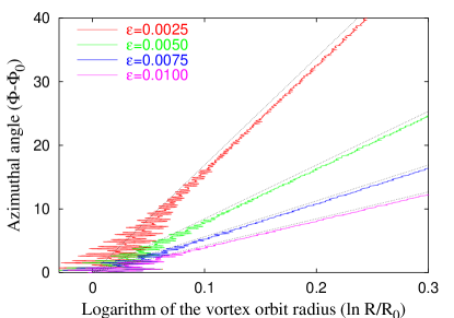
Figure 2: (Color online) Azimuthal angle $\Phi$ of the vortex position as a function of the logarithm of the radial position $R$ for four different values of the damping $\varepsilon$. The lattice radius is $L=20a\approx 11.3$.

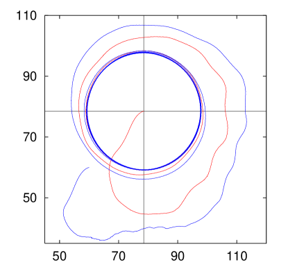
Figure 3: (Color online) Two trajectories of a vortex from simulations of the many-spin model (1)–(3), on a lattice of radius $L=78a\approx 44$, with a rotating field ($\nu=0.125$, $b=0.002$). For this field, all trajectories converge to the same circle independently of the vortex’s initial position, provided it is not too close to the system border.

To study the vortex dynamics in the presence of the rotating field, we extend the simulations described in Ref. Zagorodny et al., 2003. There we investigated the dynamics of the out–of–plane structure of the vortex, focusing on the phenomenon of switching, which occurs when $\nu p<0$. Here we consider vortices with positive polarity $p=1$ and $\nu>0$ so that no switching occurs.

For simplicity we fixed the damping $\varepsilon=0.01$ in (3) and varied the parameters $(b,\nu,L)$. We checked that the effects reported here occur for a range of anisotropies and damping around these values. Given a combination of the parameters ($\nu$,$b$) of the field, the radius $L$ of the system and the damping $\varepsilon$, we have observed that either the vortex escapes from the system through the border or it stays inside for all times. In the latter case, it can approach a limit cycle for a broad range of the field parameters. Fig. 3 shows two vortex trajectories starting from different positions and converging to the same circle. When the limit cycle exists, its basin of attraction is very large as can be seen by starting the vortex at different positions and seeing it converge to the same circle. In other words, the system keeps no memory of the initial position of the vortex.

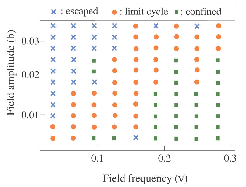
Figure 4: (Color online) Diagram of types of trajectories in the $(\omega,B)$ parameter plane corresponding in the $(\nu,b)$ plane to the range $0<\nu<0.3$ and $0<b<0.033$. The radius of the system is $L=36a\approx 20$. The term “confined” means that no limit cycle was reached, though the vortex stayed inside the system, during the time of observation $\tau\lesssim 6400$.

To exist, the limit cycle needs both magnetic field and damping: once it is attained, switching off or changing either of them destroys immediately the circular trajectory. For fixed $\nu$ and $L$, when the intensity $b$ is not large enough, damping dominates and the vortex escapes from the system following a spiral, as explained in the previous Section. If $b$ is too large, the vortex will also escape due to an effective drift force caused by the field, which changes its direction slowly enough, relative to the movement of the vortex. This is the case when the frequency is very small, such that the field is practically static. If both the intensity and the frequency are too large, the field will destroy the excitation creating many spin waves and also new vortices can be generated from the boundary. Many seemingly chaotic trajectories can be observed for high values of field parameters. To determine the limit cycle, the value of the damping is not as critical as the field parameters. For example, increasing the damping up to five times its value ($\varepsilon=0.002$ to $0.01$) did not change significantly the limit cycle shown in Fig. 3 but only accelerated the reaching of it. At this point note that there is no resonant absorption of the energy in the ac field unlike the predictions of Ref. Usov and Kurkina, 2002. The field just drives the vortex with the frequency $\Omega$, which is always lower than the frequency $\omega$ of the ac field.

All these extreme cases constrain the size and shape of the regimes where circular limit–trajectories appear in the space of field parameters $(\nu,b)$. In Fig. 4 we show for a system radius $L=36a$ this parameter plane and point out where the vortex escapes or gives rise to a limit cycle or confined orbit. Similarly to what we found in the study of switching, Zagorodny et al. (2003) we also find “windows”, i.e. events which are not expected in a particular region (for instance, the point $(\nu=0.1,b=0.02)$ in the diagram). The zoom–in of any region of the diagram containing windows shows again a similar behavior. We can also observe that the vortex is sensitive to small variations of the field parameters, and that its behavior is not monotonous (follow for example the line $b=0.025$ for increasing frequencies).

When $L$ is varied, there can appear “windows” where there is no limit cycle. For example for $L=36a$, $\nu=0.1$, $b=0.02$ the vortex escapes from the system, while for $L=24a,30a$, on one side and $L=42a,48a,54a,\cdots$ , on the other side, the vortex reaches a limit cycle.

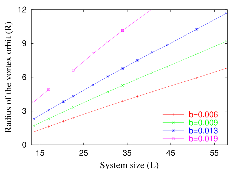
Figure 5: (Color online) Radius of the vortex orbit $R$ vs. the system radius $L$, in the circular limit cycle, for a fixed field frequency $\nu=0.094$ and several amplitudes $b$. The lines are there to guide the eye. Here and in the next figures $R$ and $L$ are given in units of $l_{0}$.

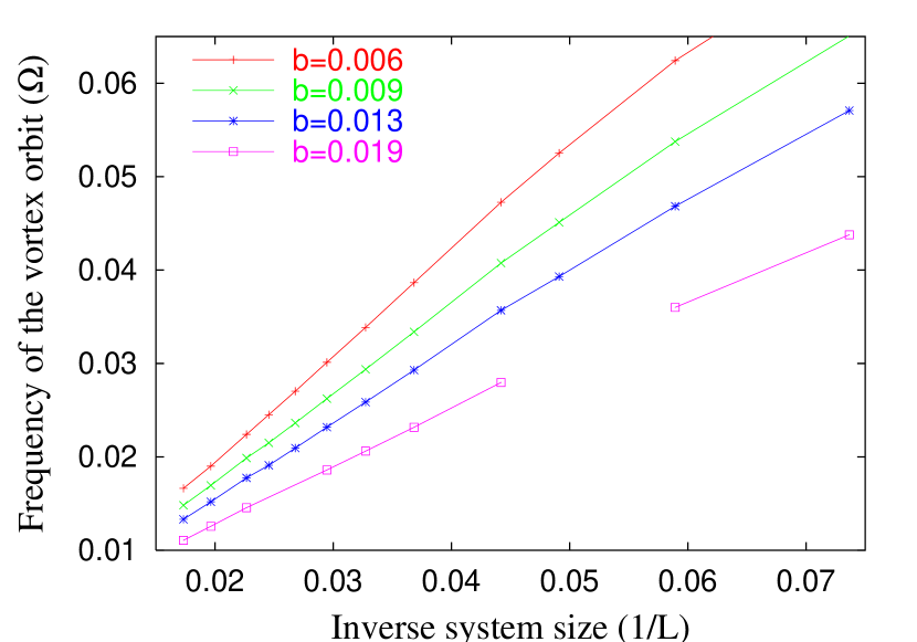
Figure 6: (Color online) Frequency of the vortex orbit $\Omega$ vs. the inverse system radius $1/L$, in the circular limit cycle, for a fixed field frequency $\nu=0.094$ and several amplitudes $b$.

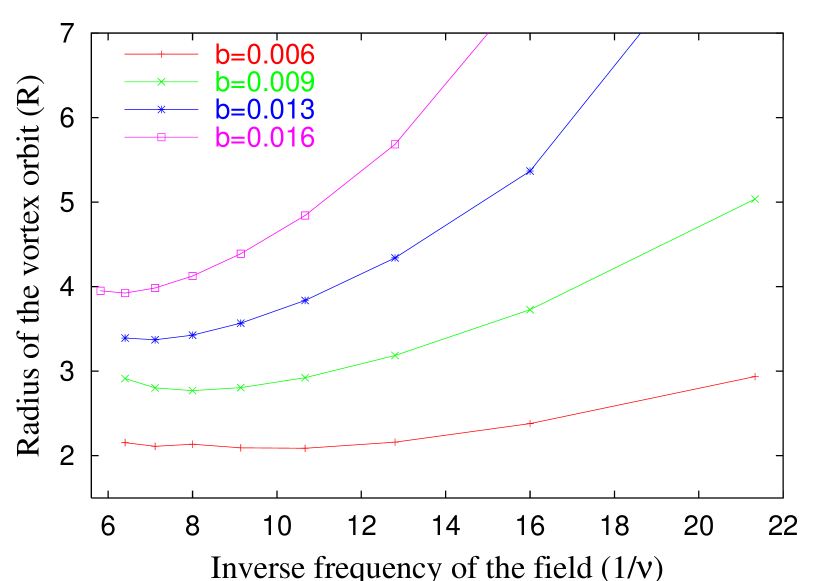
Figure 7: (Color online) Radius of the vortex orbit $R$ vs. the inverse $1/\nu$ of the frequency $\nu$ of the rotating magnetic field for four different amplitudes of the field. The radius of the system is $L=36a\approx 20$.

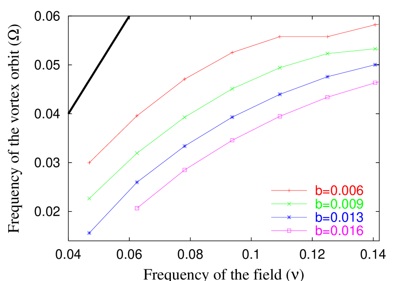
Figure 8: (Color online) Frequency of the vortex orbit $\Omega$ vs. the frequency $\nu$ of the rotating magnetic field for four different amplitudes of the field. The diagonal is plotted in the upper left corner. The radius of the system is $L=36a\approx 20$.

In the rest of this work we will concentrate on the circular limit cycle. Figs. 5 and 6 show the dependence of the vortex radial position $R$ and azimuthal frequency $\Omega$ as a function of the system radius $L$ for a fixed field frequency $\nu=0.094$ and four amplitudes $b$. The linear dependence of $R$ on the system size $L$ is very clear from Fig. 5 for the whole range $11<L<56$. Fig. 6 shows the frequency $\Omega$ of the vortex orbit as a function of $1/L$. The dependence is linear for $L>30$ but not for smaller $L$ indicating a possible size effect. The points missing in the two figures for $L=20$ and $b=0.0187$ correspond to a vortex escaping from the system.

For a fixed system size $L$ the features of the limit cycle depend on the values of the field frequency $\nu$ and amplitude $b$. In Fig. 7 we plot the radius $R$ of the limit cycle as a function of the inverse $1/\nu$ of the frequency of the applied field. For large frequencies one can see that the radius tends to a constant which is proportional to the amplitude $b$. For low frequencies the radius increases sharply. In this case damping plays a larger role than mentioned above.

In Fig. 8 we plot the frequency $\Omega$ of the orbital motion of the vortex as a function of the field frequency $\nu$ for four values of the field amplitude $b$. The diagonal is shown on the upper left corner of the picture and indicates that $\Omega\ll\nu$.

a) $\nu=0.25,\;b=0.0025$
b) $\nu=0.28,\;b=0.016$

Figure 9: Two different kinds of confined vortex trajectories that are not circular, occurring for large field amplitudes and frequencies. In the top panel the radial position $R(t)$ of the vortex is periodic while it is chaotic in the bottom panel

Although most trajectories which converge to limit cycles end up in a circular orbit around the center of the system, we have observed a few cases of a limit cycle that is not circular as shown in Fig. 9 a). Some chaotic confined trajectories can also be found as shown in the bottom panel of Fig. 9 b).

V Theoretical description of the vortex motion with rotating field

To describe analytically the observed vortex dynamics, a standard procedure is to derive Thiele–like equations, as it was done in Sec. III without field. Due to the field there appears the following Zeeman term in the total energy (see Appendix C for details):

$$V(\tau)\approx\pi bRL\cos\left(\Phi-\nu\tau\right).$$ (30)

When the vortex reaches the limit cycle, the total energy is constant. We have checked this fact in our simulations, calculating the power–dissipation relation (49). For a vortex, which moves according to the Thiele Ansatz, the power–dissipation relation (16) takes the form:

$$\frac{d\mathscr{E}}{d\tau}=-\pi\eta\dot{\bm{R}}^{2}+\pi b\nu RL\sin\left(\Phi-\nu\tau\right).$$

The energy can tend to a constant value only when $\dot{\Phi}=\nu$, so the frequency of the vortex motion should be equal to the driving frequency. Thus the standard Thiele approach cannot provide the circular motion of the vortex with the orbit frequency $\Omega<\nu$ we have observed in our simulations, see previous section. The reason is that the field excites low–frequency quasi–Goldstone modes Gaididei et al. (2000); Zagorodny et al. (2003), which can couple with the translation mode Kovalev and Prilepsky (2003). Therefore it is not correct to describe the vortex as a rigid particle and it is necessary to take into account the internal vortex structure.

To describe the approach to the limit cycle we now generalize the collective variable theory to take into account an internal degree of freedom of the vortex. Because the magnetic field changes the $z$ component of the magnetization and generates a new ground state, it is natural to include into the $m$ field an additional degree of freedom. To comply with the new ground state (15) we add to the $\phi$–field (20b) a time dependent phase $\Psi(\tau)$ describing homogeneous spin precession. $\Psi(\tau)$ can be understood as the generalization of an arbitrary constant phase which could be added in Eq. (20b) without changing the dynamics. However, this constant phase does influence the dynamics if there is a constant in–plane magnetic field, which breaks the rotational symmetry in the xy–plane Gouvêa et al. (1990).

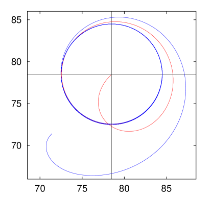
Figure 10: (Color online) Two trajectories of a vortex from the collective variable Eqs. (37), starting from different initial positions. Red line: $R(0)=a$, $\Phi(0)=5\pi/4$, $\Psi(0)=\pi/4$. Blue line: $R(0)=10a$, $\Phi(0)=5\pi/4$, $\Psi(0)=\pi/4$. Other parameters: $b=0.002$, $\nu=0.125$, $\varepsilon=0.01$, and $\delta=0.08$. System radius: $L=78a\approx 44$.

The New Ansatz that we choose is

$$m(z,\tau) =\cos\theta\left(\frac{\left|z-Z(\tau)\right|}{l(\tau)}\right),$$ (31a)

$$\phi(z,\tau) =\arg\Big{(}z-Z(\tau)\Big{)}-\arg\Big{(}z-Z_{I}(\tau)\Big{)}$$

$$\,+\arg Z(\tau)\,+\,\Psi(\tau),$$ (31b)

which describes a mobile vortex structure like (20), but including a precession of the spins as a whole, through a time–dependent phase $\Psi(\tau)$ and a dynamics of the vortex core, through the core width $l(\tau)$. The latter allows a variation of the $z$–component of the magnetization. We will see that in the Lagrangian the two variables $l$ and $\Psi$ are conjugate to each other so that one needs to introduce them together.

We find it convenient to use in the following, instead of $l(\tau)$, the $z$–component of the total spin,

$$M(\tau)=\frac{1}{\pi}\int\!\!d^{2}x\,m(z,\tau)=M_{0}l^{2}(\tau),$$ (32)

which is related to the total number of “spin deviations” or “magnons”, bound in the vortex. Kosevich et al. (1990) Here $M_{0}$

$$M_{0}=2\int_{0}^{\infty}\!\!{\rho}d{\rho}\cos\theta({\rho})\approx 2.75$$ (33)

is related to the characteristic number of magnons bound in the static vortex. Note that without dissipation and for zero field, $M$ is conserved. The field excites an internal dynamics, changing the number of bound magnons and the total spin $M$.

To construct effective equations we use the same variational technique as in Section III. Besides the “vortex coordinates” $\{R,\Phi\}$, we consider two “internal variables” $\{M,\Psi\}$ so that our set of collective variables is

$$X_{i}=\left\{R(\tau),\Phi(\tau),M(\tau),\Psi(\tau)\right\}.$$ (34)

One can derive the effective Lagrangian of the system by inserting ansatz (31) into the full Lagrangian (11), and calculating the integrals, see Appendix C for details:

$$\begin{split}{\mathscr{L}\over\pi}=M\dot{\Psi}-R^{2}\dot{\Phi}-\ln\frac{L^{2}-R^{2}}{L}+\frac{1}{2}\left(\ln\frac{M}{M_{0}}-\frac{M}{M_{0}}\right)-bLRf\left(\tfrac{R}{L}\right)\cos(\Phi+\Psi-\nu\tau).\end{split}$$ (35)

In the same way one can derive an effective dissipative function

$${\mathscr{F}\over\pi}=\frac{\varepsilon}{2}\Biggl{[}\left(\dot{R}^{2}+R^{2}\dot{\Phi}^{2}\right)\left(C_{1}+\frac{1}{2}\ln(L^{2}-R^{2})-\frac{1}{2}\ln\frac{M}{M_{0}}\right)+\dot{\Psi}^{2}\left(L^{2}-\frac{M}{M_{0}}\right)+2R^{2}\dot{\Phi}\dot{\Psi}+\frac{C_{2}\dot{M}^{2}}{MM_{0}}\Biggr{]},$$ (36)

where the constants $C_{1}$ and $C_{2}$ are introduced in (62) and (72), respectively. From the Euler–Lagrange equations (26) for the set of variables (34) we obtain finally

$$\dot{R} =\frac{\varepsilon R}{2}\left[\dot{\Phi}\left(C_{1}+\frac{1}{2}\ln(L^{2}-R^{2})-\frac{1}{2}\ln\frac{M}{M_{0}}\right)+\dot{\Psi}\right]-\frac{bL}{2}f\left(\tfrac{R}{L}\right)\sin\big{(}\Phi+\Psi-\nu\tau\big{)},$$ (37a)

$$\dot{\Phi} =\frac{1}{L^{2}-R^{2}}-\frac{\varepsilon\dot{R}}{2R}\left(C_{1}+\frac{1}{2}\ln(L^{2}-R^{2})-\frac{1}{2}\ln\frac{M}{M_{0}}\right)-\frac{bL}{2R}g\left(\tfrac{R}{L}\right)\cos\big{(}\Phi+\Psi-\nu\tau\big{)},$$ (37b)

$$\dot{M} =-\varepsilon\left[R^{2}\dot{\Phi}+\dot{\Psi}\left(L^{2}-\frac{M}{M_{0}}\right)\right]+bLRf\left(\tfrac{R}{L}\right)\sin\big{(}\Phi+\Psi-\nu\tau\big{)},$$ (37c)

$$\dot{\Psi} =\frac{1}{2}\left(\frac{1}{M_{0}}-\frac{1}{M}\right)+\varepsilon C_{2}\frac{\dot{M}}{MM_{0}}.$$ (37d)

To integrate numerically the differential algebraic system (37), one needs to solve at each step a linear system; we used the MAPLE software map which includes such a facility. The set of Eqs. (37) describes the main features of the observed vortex dynamics, and yields the circular limit cycle for the trajectory of the vortex center, see Fig. 10. Let us note that Eqs. (37a) and (37b) reduce to the Thiele equations for the coordinates $(R,\Phi)$ of the vortex center when $M$ and $\Psi$ are omitted and in this case no stable closed orbit is possible. Only including the internal degrees of freedom $(M,\Psi)$ one can obtain a stable limit cycle.

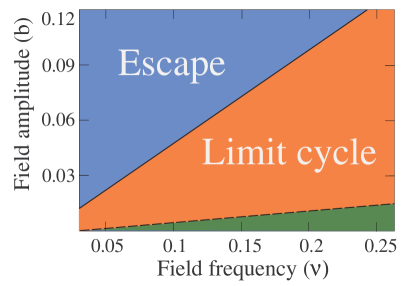
Figure 11: (Color online) The two types of trajectories observed in the $(\nu,b)$ field parameter plane for the collective variable Eqs. (37). The parameters are $\varepsilon=0.01$, $\delta=0.08$ and system radius $L=36a\approx 20$.

In the parameter plane $(\nu,b)$ shown in Fig. 11 we indicate the two main types of trajectories found by numerical integrating Eqs. (37). Vortex trajectories converge to a limit cycle only for $b\lesssim\nu/2$ (red domain). When the amplitude of the rotating field $b$ lies above the critical curve, the vortex escapes from the system along a spiral trajectory (blue domain). The model has no lower boundary for the limit cycle. However when the amplitude of the field lies below the critical curve (dashed line in Fig. 11), the radius of the vortex orbit can become less than the lattice constant (green domain). In this case discreteness effects are important for the spin system, so the model can no longer be adequate.

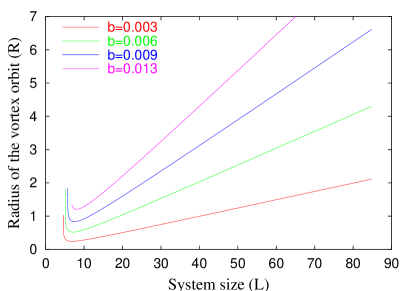
Figure 12: (Color online) Radius of the vortex orbit $R$ vs. the system size $L$, in the circular limit cycle for the collective variable Eqs. (37) for a field frequency $\nu=0.06$. The other parameters are the same as in Fig. 11.

In Fig. 12 we show the radius of the vortex orbit $R$ on the circular limit cycle as a function of the system size $L$, obtained from the numerical solution of Eqs. (37). Notice the linear dependence $R\propto L$ similar to the one observed in the numerical simulations (see Fig. 5).

To analyze the main features of the model we simplify it, assuming that the vortex orbit is never close to the system border ($R\ll L$) and that the total $z$–component of the spin varies weakly so that $N\equiv(M-M_{0})/M_{0}\ll 1$. Then one can simplify the expressions for the Lagrangian and dissipative function where the common factor $\pi$ has been omitted:

$$\mathscr{L} =M_{0}N\dot{\Psi}-R^{2}\dot{\Phi}+{R^{2}\over L^{2}}-\frac{N^{2}}{4}-bRL\cos\Delta,$$ (38a)

$$\mathscr{F} =\eta\left(\dot{R}^{2}+R^{2}\dot{\Phi}^{2}\right)+\varepsilon\frac{L^{2}}{2}\dot{\Psi}^{2}+\varepsilon R^{2}\dot{\Phi}\dot{\Psi},$$ (38b)

where $\Delta\equiv\Phi+\Psi-\nu\tau$, and $\eta$ was defined in (22).

The equations of motion which result from (38) have the simple form:

$$\dot{R} =\eta R\dot{\Phi}-\frac{bL}{2}\sin\Delta+\varepsilon{R\over 2}\dot{\Psi},$$ (39a)

$$\dot{\Phi} ={1\over L^{2}}-\eta{\dot{R}\over R}-\frac{bL}{2R}\cos\Delta,$$ (39b)

$$M_{0}\dot{N} =-\varepsilon L^{2}\dot{\Psi}+bRL\sin\Delta-\varepsilon R^{2}\dot{\Phi},$$ (39c)

$$2M_{0}\dot{\Psi} =N,$$ (39d)

The set of Eqs. (39) describes two damped periodically forced oscillators, described by two couples of variables, $(R,\Phi)$ and $(N,\Psi)$. Under the action of forcing these oscillators can phase-lock and induce the limit cycle. The numerical study of Eqs. (39) reveals three different types of behaviors as a function of the field amplitude $b$ for a fixed frequency $\nu$. We choose $\nu=0.06$. For a small $b=3\cdot 10^{-4}$, the phase $\Delta$ increases linearly with time, $N$ oscillates and $R$ increases very slowly without stabilization. When the amplitude is large such as $b=0.12$, $\Delta$ tends to $-\pi$, $N$ becomes negative and then goes back to about $0$, $R$ increases indefinitely. For $b=3\cdot 10^{-4}$, $N$ tends to a positive constant, $\Delta$ tends to $\pi$ so that terms in $\dot{R}$ balance and we have the limit cycle. One can see that the dynamics of the couple $(N,\Psi)$ is fast with a typical relaxation time of about $1/\varepsilon L^{2}$ while the dynamics of the couple $(R,\Phi)$ is slow and depends on the initial position $R_{0}$. The limit cycle is obtained for $R_{0}<0.6L$, outside that range $R$ increases indefinitely.

When the solution of the system of Eqs. (39) converges to a limit cycle, we have

$$\dot{R}=\dot{N}=0,\qquad\dot{\Phi}\equiv\Omega=\text{const},\quad\dot{\Psi}=\nu-\Omega.$$ (40)

In that case we obtain the following three algebraic equations

$$2R(\nu+A\Omega) =bL\sin\Delta,$$ (41a)

$$\varepsilon L(\nu-\Omega) =bR\sin\Delta,$$ (41b)

$$-2R\Omega =bL\cos\Delta,$$ (41c)

where $A=C_{1}-1+\ln L$. Extracting the $\sin\Delta$ term from the first and second equation, we obtain the frequency of the vortex motion

$$\Omega\approx\frac{\nu}{1+AR^{2}/L^{2}}.$$ (42)

We now eliminate the sine and cosine terms from (41a) and (41c), resulting in $R\approx bL/2\Omega$. Combining with (42) one has

$$\Omega\approx\frac{\nu+\sqrt{\nu^{2}-Ab^{2}}}{2}.$$ (43)

This value is smaller than the driving frequency $\nu$ in accordance with our simulations. However, it is not proportional to $1/L$ as in the spin simulations. For the radius of the limit cycle we have finally

$$R\approx\frac{bL}{\nu+\sqrt{\nu^{2}-Ab^{2}}}\approx\frac{bL}{2\nu}.$$ (44)

The radius of the vortex orbit $R$ depends linearly on the system size in good agreement with the results of the simulation, see Section IV. It also bears the proportionality to $1/\nu$ observed in the spin dynamics.

The range of parameters, which admits limit cycle trajectories, can be estimated from the natural condition $R<L$, which gives $b<2\nu$. However, there exist stronger restrictions for the limit cycle. The solution (43) is real (not complex) only when $\nu^{2}-Ab^{2}>0$. Another limit for the parameters is obtained from the natural condition $Rl_{0}>a$ (discreteness effects are important there). Thus the range of parameters, which admits the limit cycle trajectories can be estimated as follows:

$$\begin{split}\frac{2a}{l_{0}L}<\frac{b}{\nu}<\varkappa\end{split}$$ (45)

with $\varkappa=1/\sqrt{A}=1/\sqrt{C_{1}-1+\ln L}$.

For the parameters considered in Fig. 11 $\varkappa\approx 0.48$ so that the estimate (45) agrees with the boundary $b\approx\nu/2$ shown in the figure.

From the above expressions one can estimate $\dot{\Psi}$ on the limit cycle as

$$\dot{\Psi}\approx\frac{\nu-\sqrt{\nu^{2}-Ab^{2}}}{2},$$

which shows that the change in magnetization $N=2M_{0}\dot{\Psi}$ due to the internal variables is small. It is nevertheless crucial for obtaining the limit cycle.

VI Discussion

Another way to understand the vortex dynamics is to analyze the movement of individual spins. In a set of simulations, we recorded the components of some individual spins to observe their time evolution. We consider a large enough time so that the vortex reaches the limit cycle. For the Fourier spectrum of the $z$–component of individual spins we have observed some peaks, which appear naturally with the frequency of the limit cycle $\Omega$. Every time the vortex passes close to the spins, the spins feel a lick upwards. The behavior of $\phi(\tau)$ for several spins is shown in Fig. 13. When the vortex has reached its limit cycle ie for $t>500$ the spins behave differently whether they are inside or outside the vortex orbit. Inside, $\phi$ is quite regular and increases linearly with time at a rate given by $\nu$, with $\phi\approx\varphi_{0}+\nu\tau$. This is shown by the three upper curves in Fig. 13 for $\tau>500$ which is the time taken by the vortex to settle on its orbit. Outside the orbit and for $\tau>500$, the increase of $\phi$ is more irregular as shown by the three lower curves in Fig. 13. There the Fourier spectrum of $\phi(\tau)$ has a main frequency $\omega-\Omega$ together with additional peaks at $\omega\pm n\Omega$ where $n$ is an integer.

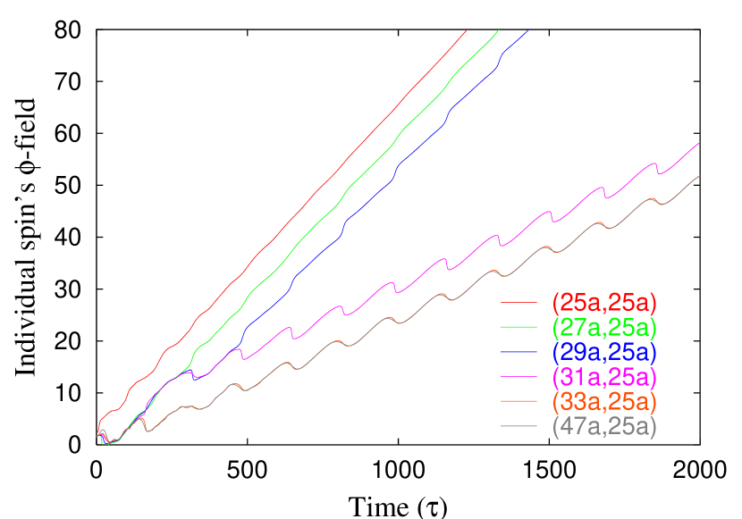
Figure 13: (Color online) Time evolution of the $\phi$–field for spins inside and outside the vortex orbit, once the vortex has reached a circular limit cycle. The parameters are $\nu=0.1$, $b=0.02$, and $L=48a\approx 27$. Inside spins ares located at $(25a,25a)$, $(27a,25a)$, $(29a,25a)$, and the outside spins are at $(31a,25a)$, $(33a,25a)$, $(47a,25a)$.

Our collective variable theory describes this effect as we show now. We assume that the vortex has reached the limit cycle so that the variables $\Phi$ and $\Psi$ fulfil the relations (40). According to the Ansatz (31), on the limit cycle the dynamical variable $\phi$ can be written as

$$\phi(z,\tau)=\varphi_{0}+\nu\tau+\arg\Big{(}z-Z(\tau)\Big{)}-\arg\Big{(}z-Z_{I}(\tau)\Big{)}.$$ (46)

We consider the vortex to be far from the boundary, i.e. $R\ll L$. Then the radius of the image–vortex trajectory is $R_{I}=L^{2}/R\gg L$, and for any $|z|<L$ the last term in Eq. (46) $\arg(z-Z_{I}(\tau))\approx\pi+\Phi(\tau)$, so

$$\phi(z,\tau)=\tilde{\varphi}_{0}+(\nu-\Omega)\tau+\arg\Big{(}z-Z(\tau)\Big{)}.$$ (47)

If we consider a spin, situated at a distance $|z|>R$, the last term in Eq. (47) describes only small oscillations on the background of the main dependence $\phi(z,\tau)=\tilde{\varphi}_{0}+(\nu-\Omega)\tau$. At the same time for a spin located at $|z|<R$, this term is decisive. Let us consider the limiting case of a spin situated near the center of the system. Then $\arg(z-Z(\tau))\approx\pi+\Phi(\tau)$, and Eq. (47) can be simply written as $\phi(z,\tau)=\varphi_{0}+\nu\tau$. Thus, the two regimes for the in–plane components of the spins are well–pronounced, which is confirmed by our simulations, see Fig. 13.

In a wide range of parameters the vortex moves along a limit circular trajectory. When the intensity of the ac field exceeds a critical value, $b>\varkappa\nu$, the vortex escapes through the boundary and annihilates. This process is important for practical applications, because vortices are known to cause hysteresis loop in magnetic nanostructures Cowburn (2002). Usually static fields are considered in the experiments and these cause a hysteresis of the $M_{x}(H_{x})$ loop, see e.g. Refs. Cowburn et al., 1999; Fernandez and Cerjan, 2000; Lebib et al., 2001; Schneider et al., 2002. The saturation field in the static regime to obtain a hysteresis is about $\omega_{0}/\gamma$ (in dimensionless units $b\sim 1$). In this article we consider an ac driving of the vortex, which causes a dynamical hysteresis, $M_{x}$ as a function of the intensity of the ac field $b$. Typical fields for vortex annihilation, $b\sim\varkappa\nu\ll 1$, are much weaker than in the static regime. It is then much easier to destabilize the vortex with an ac field than with a dc field.

Let us make some estimates. We choose permalloy (Py, $Ni_{80}Fe_{20}$) magnetic nanodots Cowburn et al. (1999); Schneider et al. (2002). The measured value of $M_{s}=\gamma SL^{2}/a^{2}=770\,G$, the exchange constant $A=JS^{2}=1.3\times 10^{-6}\,erg/cm$, and $\gamma/2\pi=2.95\,GHz/kOe$. Park et al. (2003) Typical fields of the vortex annihilation $b\sim\varkappa\nu$, which is about some tens of $Oe$.

Another important fact can be seen from Fig. 12: the vortex is unstable in small magnetic dots, the typical minimal size $L_{\text{min}}\sim 5$. For the Py magnetic dot with the magnetic length $l_{0}=5.9\,nm$, Park et al. (2003) the minimal size for the vortex state magnetic dot under weak ac driving is about $L_{\text{min}}l_{0}\sim 30\,nm$. This means that for magnetic dots with diameters less than $60\,nm$ the vortex state is unstable against the ac field giving rise to a single–domain state.

In conclusion, we developed a new collective variables approach which describes the vortex dynamics under a periodic driving, taking into account internal degrees of freedom. To our knowledge, it is the first time that an interplay between internal and external degrees of freedom, giving raise to the existence of stable trajectories, is observed in the case of 2D magnetic structures. This ansatz gives (up to a factor of 2) the radius of the limit cycle. Also the dependencies of $R$ on the system size $L$, the field amplitude, and the frequency are correct. However, the dependence of the vortex orbit frequency $\Omega$ on the system size is different from the one in the spin dynamics. Moreover, in the collective variable theory the magnetization and vortex position variables vary on very different time scales, this is not the case for the spin dynamics. Despite this we think that this collective variable approach is very general and can be employed for the self–consistent description of the dynamics of different 2D nonlinear excitations, e.g. topological solitons in 2D easy–axis magnets Sheka et al. (2001).

Appendix A Discrete spin dynamics

While Eqs. (3) are convenient for analytical consideration the presence of the time derivative on both sides makes them inconvenient for numerical simulations. Equivalent equations are obtained by forming the cross product of (3) with $\bm{S}_{\bm{n}}$ and subtracting the result from (3). In this way we get

$$\begin{split}(1+\varepsilon^{2})\frac{d\bm{S}_{\bm{n}}}{dt}=\left[\bm{S}_{\bm{n}}\times\bm{F}_{\bm{n}}\right]-\frac{\varepsilon}{S}\left[\bm{S}_{\bm{n}}\times\left[\bm{S}_{\bm{n}}\times\bm{F}_{\bm{n}}\right]\right],\end{split}$$ (48)

where $\bm{F}_{\bm{n}}=-{\partial\mathscr{H}}/{\partial\bm{S}_{\bm{n}}}$ is the total effective field; the factor $(1+\varepsilon^{2})$ is usually neglected, or absorbed into $\mathscr{H}$, giving effective constants $J$, $K$ and $B$.

From the discrete dynamics (48) one easily derives the power–dissipation relation for the total energy $\mathscr{H}=-\sum_{\bm{n}}\bm{S}_{\bm{n}}\cdot\bm{F}_{\bm{n}}$. We have

$$\frac{d\mathscr{H}}{dt} =-\sum_{\bm{n}}\bm{S}_{\bm{n}}\cdot\frac{d\bm{B}}{dt}-\sum_{\bm{n}}\bm{F}_{\bm{n}}\cdot\frac{d\bm{S}_{\bm{n}}}{dt}=-\sum_{\bm{n}}\bm{S}_{\bm{n}}\cdot\frac{d\bm{B}}{dt}$$

$$+\frac{\varepsilon}{(1+\varepsilon^{2})S}\sum_{\bm{n}}\bm{F}_{\bm{n}}\cdot\left[\bm{S}_{\bm{n}}\times\left[\bm{S}_{\bm{n}}\times\bm{F}_{\bm{n}}\right]\right]$$

and finally

$$\frac{d\mathscr{H}}{dt}=-\frac{\varepsilon}{(1+\varepsilon^{2})S}\sum_{\bm{n}}\left[\bm{S}_{\bm{n}}\times\bm{F}_{\bm{n}}\right]^{2}-\sum_{\bm{n}}\bm{S}_{\bm{n}}\cdot\frac{d\bm{B}}{dt}.$$ (49)

While the first term is always negative, it is the second term which can give rise to transients in the relaxation to equilibrium, or even the resonances, depending on the parameters of the time-dependent magnetic field.

Appendix B Collective Variable Equations without field

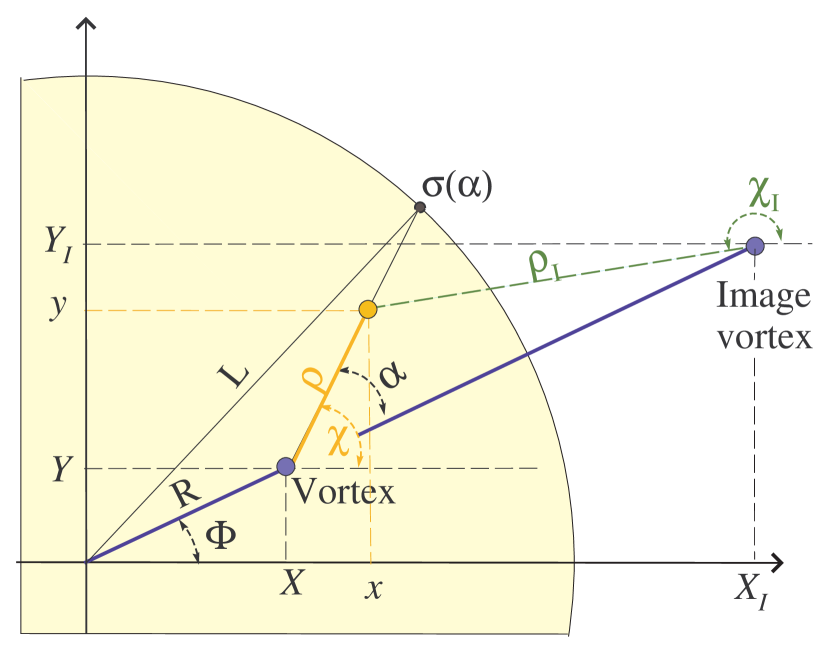
Figure 14: (Color online) Arrangement of angles in the mobile frame centered in the vortex with the coordinates $Z=X+iY=R\exp(i\Phi)$.

It is convenient to make calculations in the reference frame centered on the vortex whose axes are parallel to the standard frame

$$x-X(\tau)=\rho\cos\chi,\quad y-Y(\tau)=\rho\sin\chi~{}~{}.$$ (50)

Viewed from this point, the distance to the circular border of the system changes as a function of the azimuthal angle $\chi$, see Fig. 14. Every integral over the domain $|z|<L$ can then be calculated as

$$\int\limits_{|z|<L}\!f(\rho,\alpha)d^{2}\xi=\bigl{\langle}F(\alpha)\bigr{\rangle},\quad F(\alpha)=2\pi\!\!\int\limits_{0}^{\sigma(\alpha)}\!f(\rho,\alpha)\rho d\rho,$$

where $\alpha=\chi-\Phi$ is given by the cosine theorem

$$\sigma(\alpha)=-R\cos\alpha+\sqrt{L^{2}-R^{2}\sin^{2}\alpha},$$ (51)

and the averaging means $\bigl{\langle}F(\alpha)\bigr{\rangle}=\frac{1}{2\pi}\int_{0}^{2\pi}F(\alpha)d\alpha$. We also have the relations

$$\bm{e}_{\rho} =~{}~{}\,\bm{e}_{x}\,\cos\chi+\bm{e}_{y}\,\sin\chi,$$ (52a)

$$\bm{e}_{\chi} =-\,\bm{e}_{x}\,\sin\chi+\bm{e}_{y}\,\cos\chi,$$ (52b)

$$\bm{e}_{R} =~{}~{}\,\bm{e}_{x}\,\cos\Phi+\bm{e}_{y}\,\sin\Phi,$$ (52c)

$$\bm{e}_{\Phi} =-\,\bm{e}_{x}\,\sin\Phi+\bm{e}_{y}\,\cos\Phi.$$ (52d)

In order to derive an effective Lagrangian we start with the “microscopic” Lagrangian (11),

$$\mathscr{L}=\mathscr{G}-\mathscr{E}^{\text{int}},\qquad\mathscr{G}=-\int d^{2}\xi(1-m)\dot{\phi}.$$ (53)

We will provide all the calculations for the vortex with unit vorticity $q=1$ and positive polarity $p=1$. Using the traveling wave Ansatz (20b) in the form,

$$\phi(z,\tau)=\chi-\chi_{I}+\Phi,$$

one can calculate the time derivatives in the moving frame (50):

$$\begin{split}\dot{\chi}&=\frac{\dot{R}}{\rho}\sin\alpha-\frac{R\dot{\Phi}}{\rho}\cos\alpha.\\ \dot{\chi}_{I}&=-\frac{L^{2}\rho\dot{R}}{R^{2}\rho_{I}^{2}}\sin\alpha+\frac{L^{2}\dot{\Phi}}{R\rho_{I}^{2}}\sqrt{\rho_{I}^{2}-\rho^{2}\sin^{2}\alpha}.\end{split}$$

Here $\rho_{I}=\left\lvert z-Z_{I}(\tau)\right\rvert$, $\chi_{I}=\arg\left(z-Z_{I}(\tau)\right)$. In the main approach for $R/L\ll 1$, one can simplify an expression for $\dot{\chi}_{I}$, so finally we have

$$\begin{split}\dot{\phi}&=\left(\dot{R}\sin\alpha-R\dot{\Phi}\cos\alpha\right)\left(\frac{1}{\rho}+\frac{\rho}{L^{2}}\right).\end{split}$$ (54)

Then the gyroterm in the Lagrangian $\mathscr{G}$ gives

$$\begin{split}\mathscr{G}=&\mathscr{G}_{1}+\mathscr{G}_{2},\\ \mathscr{G}_{1}=&-\int d^{2}\xi\dot{\phi}=-2\pi\dot{R}\Bigl{\langle}[\sigma(\alpha)-L/3]\sin\alpha\Bigr{\rangle}\\ &+2\pi R\dot{\Phi}\Bigl{\langle}[\sigma(\alpha)-L/3]\cos\alpha\Bigr{\rangle},\\ \mathscr{G}_{2}=&\int d^{2}\xi m\dot{\phi}=k_{0}\dot{R}\bigl{\langle}\sin\alpha\bigr{\rangle}-k_{0}R\dot{\Phi}\bigl{\langle}\cos\alpha\bigr{\rangle},\end{split}$$

where the constant $k_{0}=2\pi\int_{0}^{\infty}\cos\theta({\rho})d{\rho}$. After averaging with account of the expressions

$$\Bigl{\langle}\sigma(\alpha)\sin\alpha\Bigr{\rangle}=0,\quad\Bigl{\langle}\sigma(\alpha)\cos\alpha\Bigr{\rangle}=-\frac{R}{2},$$ (55)

we obtain the gyroterm in the form

$$\mathscr{G}_{1}=-\pi R^{2}\dot{\Phi},\qquad\mathscr{G}_{2}=0,$$ (56)

and finally, $\mathscr{G}=-\pi R^{2}\dot{\Phi}$.

Let us calculate an effective dissipative function, starting from the “microscopic” dissipative function (12), which we cut into two terms, $\mathscr{F}=\mathscr{F}_{1}+\mathscr{F}_{2}$ with

$$\mathscr{F}_{1}=\frac{\varepsilon}{2}\int\!d^{2}\xi\ \frac{{\dot{m}}^{2}}{1-m^{2}},\quad\mathscr{F}_{2}=\frac{\varepsilon}{2}\int\!d^{2}\xi\ (1-m^{2}){\dot{\phi}}^{2}.$$

The time derivative of the $m$–field can be easily calculated in the moving frame (50), using the traveling wave Ansatz (20)

$$\dot{m}=\theta^{\prime}\sin\theta\left(\dot{R}\cos\alpha+R\dot{\Phi}\sin\alpha\right).$$ (57)

Calculating integrals for $\mathscr{F}_{1}$ with account of (57), we derive:

$$\mathscr{F}_{1}=\frac{\varepsilon\pi}{2}k_{1}\left(\dot{R}^{2}+R^{2}\dot{\Phi}^{2}\right),$$ (58)

where $k_{1}=\int_{0}^{\infty}{\theta}^{\prime 2}({\rho}){\rho}d{\rho}$. In the same way we can derive $\mathscr{F}_{2}$, taking into account $\dot{\phi}$ from Eq. (54),

$$\begin{split}\mathscr{F}_{2}&={\varepsilon\pi}\Biggl{(}\dot{R}^{2}\Bigl{\langle}(k_{2}+\ln\sigma)\sin^{2}\alpha\Bigr{\rangle}\\ &+R^{2}\dot{\Phi}^{2}\Bigl{\langle}(k_{2}+\ln\sigma)\cos^{2}\alpha\Bigr{\rangle}\\ &-R\dot{R}\dot{\Phi}\Bigl{\langle}(k_{2}+\ln\sigma)\sin 2\alpha\Bigr{\rangle}\Biggr{)},\\ k_{2}&=\frac{5}{4}+\int_{0}^{1}\frac{\sin^{2}\theta({\rho})}{{\rho}}d{\rho}-\int_{1}^{\infty}\frac{\cos^{2}\theta({\rho})}{{\rho}}d{\rho}.\end{split}$$ (59)

Using the averages

$$\begin{split}&\Bigl{\langle}\sin^{2}\!\alpha\ \ln\sigma(\alpha)\Bigr{\rangle}=\Bigl{\langle}\cos^{2}\!\alpha\ \ln\sigma(\alpha)\Bigr{\rangle}\\ &=\frac{1}{2}\Bigl{\langle}\ln\sigma(\alpha)\Bigr{\rangle}=\frac{1}{4}\ln\left(L^{2}-R^{2}\right)\end{split}$$ (60)

we calculate the dissipative function in the form

$$\mathscr{F}=\frac{\varepsilon\pi}{2}\left[C_{1}+\frac{1}{2}\ln(L^{2}-R^{2})\right]\left(\dot{R}^{2}+R^{2}\dot{\Phi}^{2}\right).$$ (61)

Here the constant $C_{1}=k_{1}+k_{2}$,

$$\begin{split}C_{1}&=\frac{5}{4}+\int_{0}^{1}\frac{\sin^{2}\theta({\rho})}{{\rho}}d{\rho}-\int_{1}^{\infty}\frac{\cos^{2}\theta({\rho})}{{\rho}}d{\rho}\\ &+\int_{0}^{\infty}{\theta}^{\prime 2}({\rho}){\rho}d{\rho}\approx 2.31.\end{split}$$ (62)

Supposing that the vortex is not close to the boundary, i.e. $R\ll L$, we obtain the effective dissipative function in the form (25).

Appendix C Collective Variable Equations with field

First we calculate an effective Zeeman energy for the standard Thiele–like motion of the vortex. Inserting the traveling wave Ansatz (20) into the “microscopic” Zeeman energy (6), and calculating the integrals, we get the effective energy in the form:

$$V(\tau) =-\frac{1}{2}b\int_{0}^{2\pi}d\chi\left[\sigma^{2}(\chi-\Phi)-c_{1}\right]\cos(\phi-\nu\tau)$$

$$=\pi bRLf\left(\tfrac{R}{L}\right)\cos\left(\Phi-\nu\tau\right),$$ (63)

where

$$f(x)=\frac{4}{3\pi}\left[E(x)\left(\frac{1}{x^{2}}+1\right)-K(x)\left(\frac{1}{x^{2}}-1\right)\right],$$ (64)

where $E(x)$ and $K(x)$ are elliptical integrals. When the vortex is far from the boundary, which is the case of interest, one can expand this function into the series, $f(x)\approx 1-{x^{2}}/{8}$. In the main approach it leads to the Zeeman term in the form (30). The corresponding magnetic force

$$\begin{split}\bm{F}_{h}=-\bm{\nabla}_{\!\!\bm{R}}V&=\bm{e}_{\!R}\,\pi bLg\left(\tfrac{R}{L}\right)\cos\left(\Phi-\nu\tau\right)\\ &-\bm{e}_{\!\chi}\,\pi bRLf\left(\tfrac{R}{L}\right)\sin\left(\Phi-\nu\tau\right),\end{split}$$ (65)

where the function

$$\begin{split}g(x)&=f(x)+xf^{\prime}(x)\\ &=\frac{4}{3\pi}\left[K(x)\left(\frac{1}{x^{2}}-1\right)-E(x)\left(\frac{1}{x^{2}}-2\right)\right].\end{split}$$ (66)

For $x\ll 1$ it has the following expansion $g(x)\approx 1-{3x^{2}}/{8}$.

Let us calculate the same Zeeman energy using the new Ansatz (31). One can derive a Zeeman term similar to (C)

$$V(\tau)=\pi bRLf\left(\tfrac{R}{L}\right)\cos\left(\Phi+\Psi-\nu\tau\right).$$ (67)

Besides this direct influence on the system, the magnetic field also changes the gyroterm in the effective Lagrangian, and the energy of the system. These changes result from the internal motion of the vortex through $l(\tau)$, and from the uniform spin precession through $\Psi(\tau)$. This does not change the gyroterm $\mathscr{G}_{1}$, which has the same form as in (56), but there appears the contribution $\mathscr{G}_{2}=M\dot{\Psi}$. This can be easily calculated with account of the time derivative

$$\dot{\phi}=\dot{\Psi}+\left(\dot{R}\sin\alpha-R\dot{\Phi}\cos\alpha\right)\left(\frac{1}{\rho}+\frac{\rho}{L^{2}}\right).$$ (68)

The total energy functional (9) can be written in the form $\mathscr{E}=\mathscr{E}_{1}+\mathscr{E}_{2}+\mathscr{E}_{3}+V$ with

$$\mathscr{E}_{1} =\frac{1}{2}\int d^{2}\xi\frac{(\bm{\nabla}m)^{2}}{1-m^{2}}=k_{1}\pi,$$ (69a)

$$\mathscr{E}_{2} =\frac{1}{2}\int d^{2}\xi(1-m^{2})(\bm{\nabla}\phi)^{2}\approx\pi\ln\frac{L^{2}-R^{2}}{l(\tau)L},$$ (69b)

$$\mathscr{E}_{3} =\frac{1}{2}\int d^{2}\xi\ m^{2}=\frac{\pi l^{2}(\tau)}{2}.$$ (69c)

The term $\mathscr{E}_{2}$, which describes the interaction between the vortex and its image, can be derived from (23), simply replacing $l_{0}$ by $l(\tau)$. In the last anisotropy term $\mathscr{E}_{3}$ we have used the relation $\int_{0}^{\infty}\cos{\theta}^{2}({\rho}){\rho}d{\rho}=1/2$, see Ref. Ivanov and Sheka, 1995. Combining all terms of the Lagrangian and omitting the constant term $\mathscr{E}_{1}$, one obtains the effective Lagrangian of the system (35).

The dissipative function contains two dynamical contributions. The first one is due to the time dependence of the $m$–field:

$$\dot{m}=\frac{\theta^{\prime}\sin\theta}{l(\tau)}\left(\frac{\dot{M}}{2M}\rho+\dot{R}\cos\alpha+R\dot{\Phi}\sin\alpha\right).$$ (70)

This term $\mathscr{F}_{1}$ can be derived in way similar to (58):

$$\mathscr{F}_{1} =\frac{\varepsilon\pi}{2}\left(k_{1}\dot{R}^{2}+k_{1}R^{2}\dot{\Phi}^{2}+\frac{C_{2}{\dot{M}}^{2}}{MM_{0}}\right),$$ (71)

$$C_{2} =\frac{1}{2}\int_{0}^{\infty}{\theta}^{\prime 2}({\rho}){\rho}^{3}d{\rho}\approx 0.48.$$ (72)

To calculate the second term $\mathscr{F}_{2}$ we use $\dot{\phi}$ from Eq. (68) and obtain

$$\begin{split}\mathscr{F}_{2}=\frac{\varepsilon\pi}{2}\Biggl{\{}&\left(\dot{R}^{2}+R^{2}\dot{\Phi}^{2}\right)\left[k_{2}+\frac{1}{2}\ln\frac{L^{2}-R^{2}}{l^{2}(\tau)}\right]\\ &+\dot{\Psi}^{2}\left[L^{2}-l^{2}(\tau)\right]+2R^{2}\dot{\Phi}\dot{\Psi}\Biggr{\}}.\end{split}$$ (73)

The total effective dissipative function $\mathscr{F}=\mathscr{F}_{1}+\mathscr{F}_{2}$ has the form (36).

References

- Mertens and Bishop (2000) F. G. Mertens and A. R. Bishop, in Nonlinear Science at the Dawn of the 21th Century, edited by P. L. Christiansen, M. P. Soerensen, and A. C. Scott (Springer–Verlag, Berlin, 2000).
- Mertens et al. (1989) F. G. Mertens, A. R. Bishop, G. M. Wysin, and C. Kawabata, Phys. Rev. B 39, 591 (1989).
- Wiesler et al. (1989) D. D. Wiesler, H. Zabel, and S. M. Shapiro, Physica B 156–157, 292 (1989).
- Shinjo et al. (2000) T. Shinjo, T. Okuno, R. Hassdorf, K. Shigeto, and T. Ono, Science 289, 930 (2000).
- Cowburn et al. (1998) R. P. Cowburn, A. O. Adeyeye, and M. E. Welland, Phys. Rev. Lett. 81, 5414 (1998).
- Cowburn et al. (1999) R. P. Cowburn, D. K. Koltsov, A. O. Adeyeye, M. E. Welland, and D. M. Tricker, Phys. Rev. Lett. 83, 1042 (1999).
- Pulwey et al. (2001) R. Pulwey, M. Rahm, J. Biberger, and D. Weiss, IEEE transactions on magnetics 37, 2076 (2001).
- Gubbiotti et al. (2002) G. Gubbiotti, G. Carlotti, F. Nizzoli, R. Zivieri, T. Okuno, and T. Shinjo, IEEE Transactions On Magnetics 38, 2532 (2002).
- Park et al. (2003) J. P. Park, P. Eames, D. M. Engebretson, J. Berezovsky, and P. A. Crowell, Phys. Rev. B 67, 020403(R) (2003).
- Fernandez and Cerjan (2000) A. Fernandez and C. J. Cerjan, J. Appl. Phys. 87, 1395 (2000).
- Raabe et al. (2000) J. Raabe, R. Pulwey, R. Sattler, T. Schweiboeck, J. Zweck, and D. Weiss, J. Appl. Phys. 88, 4437 (2000).
- Lebib et al. (2001) A. Lebib, S. P. Li, M. Natali, and Y. Chen, J. Appl. Phys. 89, 3892 (2001).
- Hubert and Schäfer (1998) A. Hubert and R. Schäfer, Magnetic Domains (Springer–Verlag, Berlin, 1998).
- Cowburn (2002) R. P. Cowburn, J. Magn. Magn. Mater. 242–245, 505 (2002).
- Skomski (2003) R. Skomski, J. Phys. C 15, R841 (2003).
- Guslienko et al. (2001) K. Y. Guslienko, V. Novosad, Y. Otani, H. Shima, and K. Fukamichi, Phys. Rev. B 65, 024414 (2001).
- Schneider et al. (2002) M. Schneider, H. Hoffmann, S. Otto, T. Haug, and J. Zweck, J. Appl. Phys. 92, 1466 (2002).
- Pokhil et al. (2000) T. Pokhil, D. Song, and J. Nowak, J. Appl. Phys. 87, 6319 (2000).
- Demokritov et al. (2001) S. O. Demokritov, B. Hillebrands, and A. N. Slavin, Physics Reports 348, 441 (2001).
- Hillebrands and Ounadjela (2002) B. Hillebrands and K. Ounadjela, eds., Spin Dynamics in Confined Magnetic Structures, vol. 83 of Topics in Applied Physics (Springer, Berlin, 2002).
- Buess et al. (2004) M. Buess, R. Hŏllinger, T. Haug, K. Perzlmaier, U. Krey, D. Pescia, M. R. Scheinfein, D.Weiss, and C. H. Back, Phys. Rev. Lett. 93, 077207 (2004).
- Choe et al. (2004) S. B. Choe, Y. Acremann, A. Scholl, A. Bauer, A. Doran, J. Stŏhr, and H. A. Padmore, Science 304, 420 (2004).
- Usov and Kurkina (2002) N. A. Usov and L. G. Kurkina, J. Magn. Magn. Mater. 242–245, 1005 (2002).
- Guslienko et al. (2002a) K. Y. Guslienko, B. A. Ivanov, V. Novosad, Y. Otani, H. Shima, and K. Fukamichi, J. Appl. Phys. 91, 8037 (2002a).
- Thiele (1973) A. A. Thiele, Phys. Rev. Lett. 30, 230 (1973).
- Thiele (1974) A. A. Thiele, J. Appl. Phys. 45, 377 (1974).
- Huber (1982) D. L. Huber, Phys. Rev. B 26, 3758 (1982).
- Nikiforov and Sonin (1983) A. V. Nikiforov and É. B. Sonin, Sov. Phys JETP 58, 373 (1983).
- Ivanov et al. (1998) B. A. Ivanov, H. J. Schnitzer, F. G. Mertens, and G. M. Wysin, Phys. Rev. B 58, 8464 (1998).
- Gaididei et al. (2000) Y. Gaididei, T. Kamppeter, F. G. Mertens, and A. R. Bishop, Phys. Rev. B 61, 9449 (2000).
- Kovalev and Prilepsky (2002) A. S. Kovalev and J. E. Prilepsky, Low Temp. Phys. 28, 921 (2002).
- Kovalev and Prilepsky (2003) A. S. Kovalev and J. E. Prilepsky, Low Temp. Phys. 29, 55 (2003).
- Zagorodny et al. (2003) J. P. Zagorodny, Y. Gaididei, F. G. Mertens, and A. R. Bishop, Eur. Phys. J. B 31, 471 (2003).
- Kovalev et al. (2003) A. S. Kovalev, F. G. Mertens, and H. J. Schnitzer, Eur. Phys. J. B 33, 133 (2003).
- Caputo et al. (2003) J. G. Caputo, J. P. Zagorodny, Y. Gaididei, and F. G. Mertens, J. Phys. A 36, 4259 (2003).
- Zagorodny et al. (2004) J. P. Zagorodny, Y. Gaididei, D. D. Sheka, J. G. Caputo, and F. G. Mertens, Phys. Rev. Lett. 93, 167201 (2004).
- Rice (1983) M. J. Rice, Phys. Rev. B 28, 3587 (1983).
- Quintero et al. (2000a) N. R. Quintero, A. Sanchez, and F. G. Mertens, Phys. Rev. Lett. 84, 871 (2000a).
- Quintero et al. (2000b) N. R. Quintero, A. Sanchez, and F. G. Mertens, Phys. Rev. E 62, 5695 (2000b).
- Gouvêa et al. (1989) M. Gouvêa, G. M. Wysin, A. R. Bishop, and F. G. Mertens, Phys. Rev. B 39, 11840 (1989).
- Mertens et al. (1997) F. G. Mertens, H. J. Schnitzer, and A. R. Bishop, Phys. Rev. B 56, 2510 (1997).
- Ivanov and Sheka (1995) B. A. Ivanov and D. D. Sheka, Low Temp. Phys. 21, 1148 (1995).
- Ivanov and Wysin (2002) B. A. Ivanov and G. M. Wysin, Phys. Rev. B 65, 134434 (2002).
- Ivanov and Yastremsky (2001) B. A. Ivanov and I. A. Yastremsky, Low Temp. Phys. 27, 552 (2001).
- Schabes and Bertram (1988) M. E. Schabes and H. N. Bertram, J. Appl. Phys. 64, 1347 (1988).
- Guslienko et al. (2002b) K. Y. Guslienko, S. O. Demokritov, B. Hillebrands, and A. N. Slavin, Phys. Rev. B 66, 132402 (2002b).
- Ivanov and Zaspel (2002) B. A. Ivanov and C. E. Zaspel, Appl. Phys. Lett. 81, 1261 (2002).
- Kamppeter et al. (1999) T. Kamppeter, F. G. Mertens, A. Sánchez, A. R. Bishop, F. Dominguez-Adame, and N. Grønbech-Jensen, Eur. Phys. J. B 7, 607 (1999).
- Gouvêa et al. (1990) M. Gouvêa, F. G. Mertens, A. R. Bishop, and G. M. Wysin, J. Phys. C 2, 1853 (1990).
- Kosevich et al. (1990) A. M. Kosevich, B. A. Ivanov, and A. S. Kovalev, Phys. Rep. 194, 117 (1990).
- (51) URL http://www.maplesoft.com.
- Sheka et al. (2001) D. D. Sheka, B. A. Ivanov, and F. G. Mertens, Phys. Rev. B 64, 024432 (2001).